HAL Id: hal-01082621
https://hal.archives-ouvertes.fr/hal-01082621
Submitted on 22 Sep 2015
HAL is a multi-disciplinary open access
archive for the deposit and dissemination of
sci-entific research documents, whether they are
pub-lished or not. The documents may come from
teaching and research institutions in France or
abroad, or from public or private research centers.
L’archive ouverte pluridisciplinaire HAL, est
destinée au dépôt et à la diffusion de documents
scientifiques de niveau recherche, publiés ou non,
émanant des établissements d’enseignement et de
recherche français ou étrangers, des laboratoires
publics ou privés.
(2004–2013): high-resolution simulations compared to
Aura MLS observations
Jayanarayanan Kuttippurath, Sophie Godin-Beekmann, Franck Lefèvre, M. L.
Santee, L. Froidevaux, Alain Hauchecorne
To cite this version:
Jayanarayanan Kuttippurath, Sophie Godin-Beekmann, Franck Lefèvre, M. L. Santee, L. Froidevaux,
et al.. Variability in Antarctic ozone loss in the last decade (2004–2013): high-resolution simulations
compared to Aura MLS observations. Atmospheric Chemistry and Physics, European Geosciences
Union, 2015, 15 (18), pp.10385-10397. �10.5194/acp-15-10385-2015�. �hal-01082621�
Atmos. Chem. Phys., 15, 10385–10397, 2015 www.atmos-chem-phys.net/15/10385/2015/ doi:10.5194/acp-15-10385-2015
© Author(s) 2015. CC Attribution 3.0 License.
Variability in Antarctic ozone loss in the last decade (2004–2013):
high-resolution simulations compared to Aura MLS observations
J. Kuttippurath1,2, S. Godin-Beekmann1, F. Lefèvre1, M. L. Santee3, L. Froidevaux3, and A. Hauchecorne1
1UPMC Université de Paris 06, UMR 8190 LATMOS-IPSL, CNRS/INSU, 75005 Paris, France 2CORAL, Indian Institute of Technology Kharagpur, Kharagpur, West Bengal, India
3JPL/NASA, California Institute of Technology, Pasadena, California, USA
Correspondence to: J. Kuttippurath ([email protected])
Received: 29 September 2014 – Published in Atmos. Chem. Phys. Discuss.: 13 November 2014 Revised: 16 August 2015 – Accepted: 17 August 2015 – Published: 22 September 2015
Abstract. A detailed analysis of the polar ozone loss
processes during 10 recent Antarctic winters is presented with high-resolution MIMOSA–CHIM (Modèle Isentrope du transport Méso-échelle de l’Ozone Stratosphérique par Ad-vection avec CHIMie) model simulations and high-frequency polar vortex observations from the Aura microwave limb sounder (MLS) instrument. The high-frequency measure-ments and simulations help to characterize the winters and assist the interpretation of interannual variability better than either data or simulations alone. Our model results for the Antarctic winters of 2004–2013 show that chemical ozone loss starts in the edge region of the vortex at equivalent latitudes (EqLs) of 65–67◦S in mid-June–July. The loss progresses with time at higher EqLs and intensifies dur-ing August–September over the range 400–600 K. The loss peaks in late September–early October, when all EqLs (65– 83◦S) show a similar loss and the maximum loss (> 2 ppmv – parts per million by volume) is found over a broad vertical range of 475–550 K. In the lower stratosphere, most winters show similar ozone loss and production rates. In general, at 500 K, the loss rates are about 2–3 ppbv sh−1(parts per bil-lion by volume per sunlit hour) in July and 4–5 ppbv sh−1in August–September, while they drop rapidly to 0 by mid-October. In the middle stratosphere, the loss rates are about 3–5 ppbv sh−1in July–August and October at 675 K. On av-erage, the MIMOSA–CHIM simulations show that the very cold winters of 2005 and 2006 exhibit a maximum loss of
∼3.5 ppmv around 550 K or about 149–173 DU over 350– 850 K, and the warmer winters of 2004, 2010, and 2012 show
a loss of ∼2.6 ppmv around 475–500 K or 131–154 DU over 350–850 K. The winters of 2007, 2008, and 2011 were mod-erately cold, and thus both ozone loss and peak loss alti-tudes are between these two ranges (3 ppmv around 500 K or 150 ± 10 DU). The modeled ozone loss values are in reason-ably good agreement with those estimated from Aura MLS measurements, but the model underestimates the observed ClO, largely due to the slower vertical descent in the model during spring.
1 Introduction
Since the early 1980s significant losses in stratospheric ozone have been observed in the Antarctic spring (WMO, 2014). The low temperatures (below 195 K) in the polar winter in-duce the formation of polar stratospheric clouds in the 15– 21 km altitude region, on which chlorine and bromine are ac-tivated; when the sun returns over the region, the chlorine-and bromine-induced catalytic ozone loss takes place. Since the 1970s, anthropogenic activities have gradually increased the concentrations of ozone-depleting substances (ODSs) in the atmosphere, including chlorine- and bromine-containing compounds, until they peaked around 2000 in the polar re-gions. The springtime ozone loss, therefore, has correspond-ingly increased since the late 1980s and was saturated by the early 1990s (WMO, 2014). In the Southern Hemisphere, the land and ocean contrast is smaller than in the Northern Hemi-sphere, and, hence, the generation and propagation of
large-amplitude planetary waves are not very effective. Therefore, the polar vortex that forms in fall and winter in the strato-sphere is relatively undisturbed and stable, and typically lasts for more than 7 (May–November) months. These dynami-cal conditions further aggravate the ozone loss in the south-ern polar vortex region. Because of the suppressed wave and dynamical disturbances, and the concomitant stability of the polar vortex, the interannual variation in Antarctic ozone loss since the 1990s has been small.
Large variability in Antarctic ozone loss has been seen in the last few years (2004–2013) relative to other winters since 1992 (e.g., Tilmes et al., 2006; Huck et al., 2007; Yang et al., 2006; Santee et al., 2008a). For instance, the winters of 2004, 2010, and 2012 were relatively warm, with minor warmings and, hence, limited ozone loss (Santee et al., 2005; de Laat and van Weele, 2011; WMO, 2014). The first fort-night of August 2005 was unusually cold and showed a high rate of ozone loss and an unprecedented ozone hole (WMO, 2014). The winter of 2006 was one of the coldest and, hence, the Antarctic vortex experienced the largest ozone hole to date (Santee et al., 2011; WMO, 2014). The winters of 2007, 2009, and 2013 were characterized by average temperatures and, hence, ozone holes of a moderate size (Tully et al., 2008; Kuttippurath et al., 2013). However, the winters of 2008 and 2011 were again very cold and characterized by large ozone holes (Tully et al., 2011; WMO, 2014). Here, we provide a detailed view of these 10 winters in relation to polar process-ing and the chemistry of ozone loss. In this study, we discuss (i) the interannual variability in ozone loss and chlorine acti-vation and (ii) horizontal, vertical, and seasonal variability in ozone loss in the Antarctic stratosphere during these (2004– 2013) winters. We use high-resolution simulations for ana-lyzing the polar processing and interannual changes in ozone loss in detail. Note that the simulations are highly resolved in the lower stratosphere (about 0.5 km between 425 and 550 K) too, to closely study the ozone loss features in those peak ozone loss altitude layers. Additionally, the past 10 winters offer a good opportunity to test the chemical and dynam-ical processes in numerdynam-ical models. Furthermore, observa-tions from the Aura microwave limb sounder (MLS) (Froide-vaux et al., 2008; Santee et al., 2008b), one of the best satel-lite instruments currently available for sampling polar vor-tices, are compared to the model results. Therefore, for the first time ozone loss and chlorine activation can be studied with high-resolution measurements that have very good spa-tial and temporal coverage inside the Antarctic vortex. Previ-ous satellite measurements were relatively limited to a small temporal and spatial area as far as high-latitude observations are concerned (e.g., Tilmes et al., 2006; Hoppel et al., 2005). While the Upper Atmosphere Research Satellite MLS (Wa-ters et al., 1999) had a similar latitudinal coverage, the fre-quency of its polar measurements was lower than that of Aura MLS (e.g., Livesey et al., 2013; Froidevaux et al., 2008). Therefore, the study with high-resolution simulations (both horizontally and vertically) together with the high-resolution
measurements offers some new insights into the polar pro-cessing and ozone loss features of the Antarctic stratosphere. In this article, the MIMOSA–CHIM (Modèle Isentrope du transport Méso-échelle de l’Ozone Stratosphérique par Advection avec CHEMie) chemical transport model (CTM) (e.g., Kuttippurath et al., 2010; Tripathi et al., 2007) is used to simulate the chemical constituents for the period 2004– 2013. The simulated results are then compared to the Aura MLS measurements. We first look at the ozone loss evolution within different equivalent latitudes (EqLs) averaged over 10 winters in Sect. 3.1. The assessment of the interannual variability in the ozone loss, chlorine activation, and ozone loss rates during the 10 (2004–2013) winters is presented in Sect. 3.2. Finally, Sect. 4 concludes with our main findings.
2 Simulations and measurements
We use the high-resolution MIMOSA–CHIM CTM for the simulations of chemical constituents (e.g., Kuttippurath et al., 2010; Tripathi et al., 2007). The model extends hor-izontally from 10◦N to 90◦S with 1◦×1◦ resolution, and there are 25 isentropic vertical levels between 350 and 950 K with a resolution of about 0.5–2 km, depending on altitude. The model is forced by European Centre for Medium-Range Weather Forecasts (ECMWF) operational analyses. The ver-tical levels of this data set have been changed from 60 to 91 levels from February 2006 to May 2013 and then to 137 levels from June 2013 onward. The chemical fields used to initialize MIMOSA–CHIM each year are obtained from a long-term simulation of the REPROBUS (Reactive Pro-cesses Ruling the Ozone Budget in the Stratosphere) CTM (Lefèvre et al., 1994) driven by the same ECMWF analyses. The REPROBUS model is equivalent to a lower-resolution version of the MIMOSA–CHIM model, with its resolution being 2×2◦. The chemical tendencies are calculated every 15 min and the output is written for every 6 h. The passive tracer is initialized only once at the beginning of the sim-ulation, and thus the ozone loss is the cumulative loss in ppmv since the beginning of the simulation. The MIMOSA– CHIM CTM uses the Middle Atmosphere Radiation Scheme (MIDRAD) (Shine, 1987). Climatological H2O and CO2, but
interactive O3 fields are used for the calculation of heating
rates. The kinetics data are taken from Sander et al. (2011) but the Cl2O2 photolysis cross sections from Burkholder
et al. (1990), with a log-linear extrapolation up to 450 nm (Stimpfle et al., 2004). These cross sections are in good agreement with the recent Cl2O2measurements by
Papanas-tasiou et al. (2009), which form the basis for the JPL 2011 recommendations (i.e., Sander et al., 2011). For each Antarc-tic winter the model was run from 1 May to 31 October.
The model has detailed polar stratospheric cloud (PSC) formation and growth and sedimentation schemes. The satu-ration vapor pressure provided by Hanson and Mauersberger (1988) and Murray (1967) is used to assume the existence
J. Kuttippurath et al.: Variability in Antarctic ozone loss 10387
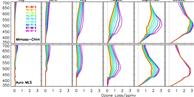
Figure 1. The 10-year (2004–2013) average monthly mean ozone loss estimated at different equivalent latitude (EqL) bins (of 2◦) from 65 to 83◦S EqL from the MIMOSA–CHIM simulations and MLS measurements. The model results are interpolated with respect to the time and location of the MLS measurements inside the vortex and then averaged for the corresponding day. The y axis represents potential temperature in K. The black dotted lines represent 0 ppmv.
of nitric acid trihydrate (NAT) and ice particles, respectively. Liquid supercooled sulfuric acid aerosols, NAT, and ice par-ticles are considered to be in equilibrium with the gas phase (Lefèvre et al., 1998). Equilibrium composition and volume of binary (H2SO4–H2O) and ternary (HNO3–H2SO4–H2O)
droplets are calculated using an analytic expression given by Carslaw et al. (1995). For NAT and ice particles, the num-ber density is set to 5 × 10⁻³cm−3, and the particle diameter is calculated within the scheme from the available volume of HNO3and H2SO4. A denitrification scheme is also
incor-porated to diagnose the sedimentation of HNO3-containing
particles. In this scheme, the NAT particles are assumed to be in equilibrium with gas phase HNO3. All three types of
NAT, ice, and liquid-aerosol particles are considered, and the sedimentation speed of the particles is calculated according to Pruppacher and Klett (2010).
We use the Aura MLS measurements version (v) 3.3 (Livesey et al., 2013) for a comparison with simulations. The ozone measurements have a vertical resolution of 2.5– 3 km over 215–0.02 hPa, and the vertical resolution of ClO measurements is about 3–3.5 km over 100–1 hPa. The time resolution of the measurements is about 3500 profiles per day. The estimated uncertainty of typical ozone and ClO re-trievals is about 5–10 and 10–20 %, respectively (Livesey et al., 2013; Santee et al., 2008a; Froidevaux et al., 2008). For a comparison with the measurements, the model results (6 h output) are interpolated to the measurement locations.
3 Results and discussion
The passive tracer method is applied to compute the ozone loss from the simulations and measurements. This requires the simulation of passive ozone (or a passive model tracer), i.e., ozone simulations without interactive chemistry. The ozone loss is computed as the difference between the mod-eled passive odd-oxygen tracer (defined as the sum of O3,
O(1D) and O3(P)) and measured or simulated ozone. To de-rive the ozone loss inside the vortex, we use a vortex edge criterion of 65◦EqL. The following equation is used to de-rive the vortex-averaged ozone loss rates and production rates from the model results.
δO3(θ, j ) (ppbv/sh) = λeq=90 P λeq=65 δO3(θ, j, λeq) ×sh(θ, j, λeq) λeq=90 P λeq=65 sh(θ, j, λeq) , (1)
where δO3(θ, j )is the ozone loss or production averaged
within EqL (λeq) ≥ 65◦for each model vertical level (θ ) and
day (j ). δO3(θ, j, λeq) is the instantaneous ozone loss or
production calculated by the model for each grid point de-fined by latitude (φ) and longitude (ψ) for each θ and j .
sh(θ, j, λeq)is the sunlit hour, which is calculated with
re-spect to solar zenith angle < 95◦and which varies between 0 and 1 for complete darkness to full illumination. The λeq
is computed for each model grid point (θ ,φ,ψ) and for each day using potential-vorticity (PV) data.
3.1 Ozone loss: the 2004–2013 average
To elucidate various chemical ozone loss features, we ana-lyze the vertical distribution of the average loss in 2004–2013 for different EqL bins estimated from the model and MLS data from May to October and shown in Fig. 1. The EqL-based analyses extend from 65 to 83◦S in 2◦increments as calculated for the MLS measurements. A detailed discussion on the calculation of EqLs and determination of the polar vortex edge can be found in Nash et al. (1996) and references therein. The simulations show that the chemical loss starts at lower EqLs of 65–67◦S at the edge of the Antarctic vortex in May, above 600 K, as also shown by Lee et al. (2000), Godin et al. (2000), and Roscoe et al. (2012). It moves down to the lower altitudes by July, and the loss is largest at 65– 67◦S EqL. The loss continues to increase in August, with the
EqLs of 65 and 83◦S showing the largest and smallest loss,
respectively, in accordance with the increase in incidence of sunlight over the region. A clear difference in the amount of ozone loss estimated at different EqLs is well simulated. At the edge of the vortex, a maximum modeled ozone loss of 2.1 ppmv (parts per million by volume) is found around 500–550 K, while in the 70–80◦S EqL range the peak loss is found above 600 K.
The ozone loss continues through to September, when all EqLs show a large loss. The largest modeled loss is still found in the lower EqLs of 65–69◦S, reaching about 3 ppmv at 500 K. The higher EqLs (77–83◦S) show the smallest ozone loss and it peaks in the middle stratosphere (600 K), while other EqLs show their peak loss below 575 K. Above 600 K, all EqLs show a similar ozone loss of about 1.4 ppmv. The maximum loss is about 3 ppmv over 65–70◦S at 500 K,
2.5 ppmv over 70–75◦S at 550 K, 1.7 ppmv over 75–80◦S at
575 K, and 1.3 ppmv over 80–83◦S at 600 K, and thus, the al-titude of maximum loss increases with EqL up to September. As expected, the maximum ozone loss is found in October, and all EqLs show more or less the same loss (about 3 ppmv) at the peak loss altitude of around 500 K. In addition, all EqLs show a more or less similar amount of ozone loss with altitude below 500 K in October. Above 500 K, the ozone loss shows slight differences, with the largest loss occurring at the highest EqLs, unlike in months earlier than September. Note that the ozone loss presented here is the monthly mean ozone loss, not the instantaneous loss (see later analyses in Sect. 3.2.3 and 3.2.5), which explains the large ozone loss estimated for late September and October after the chlorine activation period (mid-June to mid-September). In addition, in October, the mixing processes affecting the air mass within the vortex when the ozone loss cycles are stopped also ho-mogenize the ozone distributions.
The analyses with model results below 500 K are in good agreement with those of the MLS measurements. Neverthe-less, the loss estimated from the observations is more com-pact with altitude in October, and the model–measurement differences are larger in September than in other months.
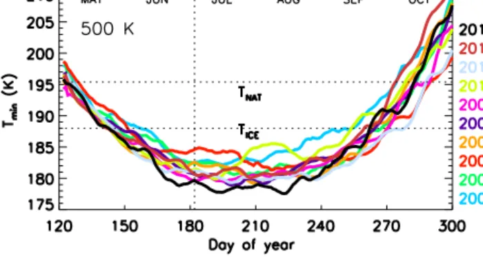
Figure 2. Evolution of polar cap (50–90◦S) minimum tempera-ture derived from the ECMWF operational analyses for each winter from 2004 to 2013 at 500 K (∼ 19 km) potential temperature. The TNATand TICEthresholds are also marked.
The comparison of ozone loss above 550 K shows that the model overestimates the ozone loss there. The ozone loss of about 0.05–0.08 ppmv that is derived from the measure-ments in May at 360–370 K is within the estimated error bars of the measurements and therefore insignificant. The differences between measurements and simulations will be discussed further in Sect. 3.2.
3.2 Interannual variations
We have discussed the general features of the measured and modeled ozone loss evolution in the Antarctic stratosphere. Now we look into the details of the interannual variations in Antarctic ozone loss. It is well-known that low temperatures initiate PSC formation, enabling chlorine activation, which then triggers ozone loss. Therefore, we first analyze the min-imum temperature and meteorological situation of each win-ter in 2004–2013. The link between the prevailing meteorol-ogy and chlorine activation of the winters is discussed in the following section, as the amount and extent of activated chlo-rine are a good indicator of the yearly changes in ozone loss. The year-to-year changes in ozone loss, i.e., the vertical pro-file of ozone loss, column ozone loss, and the instantaneous ozone loss are discussed in detail with respect to the afore-mentioned factors in the subsequent sections.
3.2.1 Meteorological conditions
Figure 2 shows the minimum polar cap (50–90◦S)
temper-ature extracted from the ECMWF operational analyses for each winter since 2004 at 500 K (∼19 km) potential tempera-ture. In general, the winters show a minimum temperature of about 179–186 K from mid-June to mid-September. Among the winters, 2004 shows relatively higher minimum temper-atures in the range of 184–200 K from August onward, al-though some days can be excluded. In 2005, the tempera-tures are relatively low and remained around 182 K in July– September, although a minor warming is evident in June.
J. Kuttippurath et al.: Variability in Antarctic ozone loss 10389
Figure 3. Vertical distribution of the vortex-averaged (defined by ≥ 65◦EqL) ClO estimated from the MIMOSA–CHIM model and MLS measurements for the Antarctic winters 2004–2013. The model results are interpolated with respect to the time and location of the MLS measurements inside the vortex and then averaged for the corresponding day. ClO data are not available for early May 2006 and late July and early August 2007. The measurements are selected for 10:00–16:00 local solar time and solar zenith angles below 89◦. Both model results and MLS data are smoothed for 7 days. The y axis represents potential temperature in K. The white dotted lines represent 500 K (∼19 km) and 675 K (∼26 km).
In 2006, the temperatures are higher (around 184 K) than in other winters in late June and July, but the September and Oc-tober temperatures (183–199 K) are very low. In 2007, 2008 and 2009, the evolution of temperature is very similar, but there are minor differences in the details, such as a sudden increase of about 181–183 K in July in 2007. In 2010, minor warmings are apparent in early August (182–186 K) and mid-September (185–190 K). The lowest mid-August to October temperatures at this level are found in 2011 as in the case of 2006, but the highest temperatures in October are found in 2012 with values of 194–212 K. In addition, the winter of 2013 shows the lowest July–August temperatures, with about
177–179 K. In brief, the winters of 2004, 2010 and 2012 can be termed warm winters (de Laat and van Weele, 2011) and 2005, 2006, 2011, and 2013 cold or very cold winters (WMO, 2014). Since the temperature evolution is between these extremes, the other winters can be called moderately cold or moderately warm. Note that the winters are catego-rized with respect to the temperature evolution at this particu-lar potential temperature, and hence the classification can be slightly different at other altitude levels. Further details about the temperature distribution and meteorology of the winters of 2010–2013 can be found in WMO (2014).
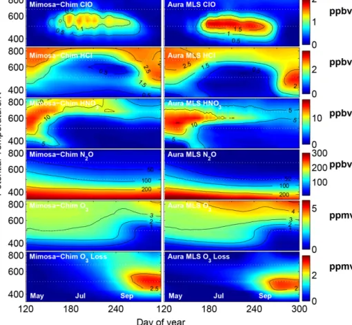
Figure 4. The vortex-averaged (defined by ≥ 65◦EqL) vertical and temporal evolution of ClO, HCl, HNO3, N2O, O3and ozone loss
from the MIMOSA–CHIM model and MLS measurements. The model results are interpolated with respect to the time and location of the MLS observations inside the vortex and then averaged for the corresponding time period. The data are the average of 10 Antarctic winters (2004–2013) and are smoothed for 7 days. ClO data are not available for early May 2006 and late July and early August 2007. The ClO measurements are selected for 10:00–16:00 for local solar time and solar zenith angles below 89◦. The y axis represents potential temperature in K and is on a logarithmic scale. The white dotted lines represent 500 K (∼19 km) and 675 K (∼26 km).
3.2.2 Activated chlorine
Figure 3 compares the simulated and measured ClO at the MLS sampling points inside the vortex, defined here by the area within 65–90◦S EqL and with a solar zenith angle (SZA) of less than 89◦, for the Antarctic winters of 2004– 2013. In MIMOSA–CHIM, relatively high chlorine activa-tion is found in 2005, when a maximum of 1.6–1.8 ppbv (parts per billion by volume) is simulated from June to late July and early August, consistent with the lower tempera-tures in that winter (WMO, 2014). The other winters show a more or less similar distribution of ClO and thus, chlorine ac-tivation, except in the warm winters of 2010 and 2012. The simulated ClO stands in contrast to the temperature struc-ture and PSC observations in each winter (Pitts et al., 2009), which showed the largest areas of PSCs in the coldest win-ters of 2005 and 2006. It should be noted that chlorine acti-vation does not depend only on temperature and the occur-rence of PSCs but also on the available chlorine reservoirs, which vary from one year to the next (Strahan et al., 2014).
However, when we examine the MLS measurements, they mostly follow the temperature history of each winter, as the observations show the strongest chlorine activation in 2005 and 2006 and the weakest in 2010 and 2012. The highest ClO values (> 1.5 ppbv) are found from July to the end of September over 450–600 K in the colder winters but around 550 K episodically in July–August in the warmer winters in the observations. Therefore, in contrast to the model results, the vortex-averaged MLS measurements display a clear in-terannual variation in the chlorine activation. These compar-isons show that the model underestimates the observed ClO over the 450–600 K range.
In order to find out the reasons for the differences between simulated and measured ClO, we compared the simulated HCl, N2O, and HNO3with the MLS observations. Figure 4
illustrates the 10-year average of the vortex mean (defined by ≥ 65◦ EqL) ClO, HCl, HNO3, N2O, O3and ozone loss
from the MIMOSA–CHIM simulations and MLS measure-ments. The N2O comparisons show that the simulated values
J. Kuttippurath et al.: Variability in Antarctic ozone loss 10391
Figure 5. Vertical distribution of the vortex-averaged (defined by ≥ 65◦EqL) ozone loss estimated for the Antarctic winters in 2004–2013. The model results are interpolated with respect to the time and location of the MLS measurements inside the vortex and then averaged for the corresponding day. Left: the ozone loss derived from the difference between the passive ozone and the chemically integrated ozone by MIMOSA–CHIM. Right: the ozone loss derived from the difference between the MIMOSA–CHIM passive ozone and the ozone measured by MLS. Both model results and MLS data are smoothed for 7 days. The y axis represents potential temperature in K. The white dotted lines represent 500 K (∼19 km) and 675 K (∼26 km).
and 100 ppbv isopleths. This bias in the simulations implies that the vertical diabatic descent in the model is slower than that deduced from MLS observations in polar spring. Con-sequently, the Cly and thus ClO in the model are relatively
smaller. Therefore, the available chlorine or HCl for conver-sion to activated ClO is smaller in the model. The HCl com-parison corroborates this feature of the simulations, as HCl is smaller in the simulations than in the measurements in early and midwinter and in late spring in the lower stratosphere. The deficiency in the vertical descent in the model has clearly affected the ozone simulations. For instance, the statistics of
the ozone comparison reveal that the differences in May are negligible at all altitudes. In June–August, the model under-estimates the measured ozone by about 0.2–0.5 ppmv below 500 K. In September–October, the model overestimates (0.2– 0.4 ppmv) the measured ozone below 450 K, with a peak at around 400 K. However, this overestimation is well be-low the peak ozone loss altitudes. Above 500 K, the model consistently underestimates the measured ozone from about 0.2 ppmv in June to 0.5–1 ppmv in August–October. Hence the differences at these altitudes are also qualitatively consis-tent with the slower vertical descent of ozone in the model.
A simulation with a different Cl2O2 recombination rate
constant (Nickolaisen et al. (2006) instead of the JPL rec-ommendation, as suggested by von Hobe et al. (2007)), was performed to test the sensitivity of the simulations and to diagnose whether the new simulations reduce the model– measurement differences. However, the ClO results did not improve significantly and hence the original simulations are presented. The HNO3comparisons also indicate that the
den-itrification in the model is overestimated, due to the equilib-rium PSC scheme of the model, as it forms large NAT par-ticles too readily, causing more sedimentation of PSCs and thus more denitrification.
Note that the relatively low model top could also influ-ence the slower descent or vertical transport in the model. A detailed discussion of the differences in measured and mod-eled ClO and HCl, chlorine partitioning in the model, and the influence of the lower model top in the simulated re-sults will be presented in a separate paper. Also, there can be small interannual differences in the diabatic descent, de-pending on the accuracy of the wind fields. These have to be kept in mind while interpreting the simulations. However, in a similar study, Santee et al. (2008a) compared the MLS measurements to SLIMCAT (Single Layer Isentropic Model for Chemistry And Transport) model (Chipperfield, 1999) re-sults and found that their simulations slightly overestimate the ClO measurements for the Antarctic winters of 2004 and 2005. They attributed these differences to the equilibrium PSC scheme of the model. In contrast, our model ClO re-sults underestimate the observations, although using a very similar PSC scheme. It suggests that even if the models use similar PSC schemes, the difference in model dynamics can induce significant changes in the simulated results. Never-theless, note that the model has performed better in northern hemispheric simulations, where the ClO simulations overes-timate the MLS measurements in the 2011 winter (Kuttippu-rath et al., 2012) but slightly underestimate them in 2005– 2010 (Kuttippurath et al., 2010).
3.2.3 Ozone loss: vertical and temporal features
Figure 5 shows the vortex-averaged ozone loss estimated from the model and MLS at the MLS sampling locations in-side the vortex in 2004–2013. As discussed in Sect. 3.1, the ozone loss onset (i.e., ozone loss > 0.5 ppmv) in the model occurs in mid-June at altitudes above 550 K and gradually moves down to the lower stratosphere by mid-August. The loss intensifies by mid-August, peaks by late September– early October and slows down thereafter as the ozone recov-ers through dynamical processes.
In the simulations, as expected, the colder winters of 2005 and 2006 show the early onset of ozone loss, in mid-June. The estimated loss is less than 0.5 ppmv above 675 K until mid-August, increases to 1–1.5 ppmv by mid-September in the lower stratosphere, and peaks at 2.5–3.6 ppmv over 450– 600 K by early October, consistent with the temporal and
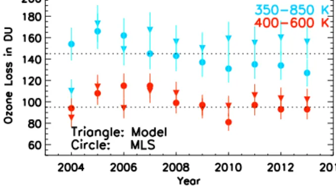
ver-Figure 6. Vortex-averaged (defined by ≥ 65◦EqL) column ozone loss computed from the MIMOSA–CHIM model simulations and MLS measurements, during the maximum ozone loss period in the Antarctic, at 350–850 K and 400–600 K for the 2004–2013 period. The estimated uncertainty of the column loss computed from both simulations and measurements is about 10 % (e.g., Kuttippurath et al., 2011).
tical extent of activated ClO in these winters. A maximum ozone loss of around 3.5 ppmv is derived around 550 K in 2005–2006 and about 3 ppmv around 500 K in 2007, 2008 and 2011. A smaller ozone loss is found in the warmer win-ters of 2004, 2010 and 2012, where the peak loss is about 2.6 ppmv, around 475 K. A similar range of ozone loss, but in a slightly broader vertical extent of 450–600 K, is simulated in 2009 and 2013. Therefore, the center of the peak ozone loss altitude (i.e., loss > 2 ppmv) also shows corresponding variations in agreement with the meteorology of the winters, as it is located around 550 K in very cold winters (e.g., 2005 and 2006), around 500 K in moderately cold winters (e.g., 2007), and around 475 K in warm winters (e.g., 2004 and 2012).
In general, the timing and vertical range of ozone loss in the simulations are similar to those of the observations. The modeled ozone loss onset is in mid-June, except for the colder winters (when it is in mid-May), as discussed pre-viously, and the loss strengthens by August–September and reaches a maximum in early to mid-October, consistent with the maxima of the observations. The large ozone losses ob-served above 550 K in September–October in the colder win-ters (e.g., 2005, 2006, 2007, 2008, and 2011) are also re-produced by the model. In contrast to the observed loss, the simulated ozone loss in 2007 is slightly higher than that of 2005, consistent with the temperature during these years at 500 K. However, the model consistently overestimates the measured ozone loss in the middle stratosphere in all years by about 0.2–0.5 ppmv in spring, as the model underestimates the measured ozone by the same amount at these altitudes, primarily due to the slower descent in the model during the period as discussed before. Therefore, the interannual vari-ations are more prominent in the measurements than in the model simulations. Note that since the same passive model
J. Kuttippurath et al.: Variability in Antarctic ozone loss 10393
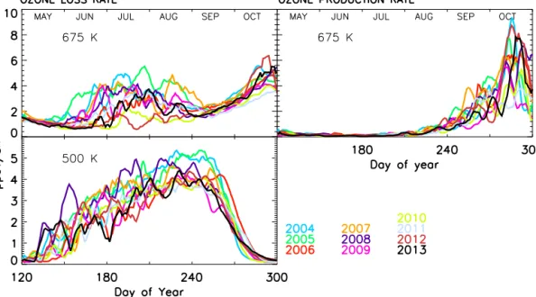
Figure 7. Vortex-averaged (defined by ≥ 65◦EqL) chemical ozone loss and production rates at 675 K (∼ 26 km) and 500 K (∼19 km) in ppbv per sunlit hour (ppbv sh−1) for the Antarctic winters 2004–2013 estimated from the MIMOSA–CHIM model simulations.
tracer affected by the slower diabatic descent in spring is used to derive ozone loss from the measurements, the mea-sured ozone loss is also overestimated. Both the simulations and measurements, however, provide consistent results for the peak ozone loss altitudes in each winter.
The ozone loss derived from the SCanning Imaging Absorption spectroMeter for Atmospheric CHartographY (SCIAMACHY) (Bovensmann et al., 1990) ozone profiles using the vortex descent method shows comparable values to that of the simulations and MLS data for the Antarctic win-ters of 2004–2008 (Sonkaew et al., 2013). There is also good agreement in peak ozone loss values (around 3–3.5 ppmv) and the differences in the altitudes of maximum loss for var-ious winters. In addition, the large loss above 500 K found in the model and MLS data is also inferred from the SCIA-MACHY measurements.
3.2.4 Partial column ozone loss
In order to gain further insights into the interannual variabil-ity in ozone loss, we now analyze the column ozone loss de-rived from simulations and measurements. Since there are also other published results available for comparisons, ana-lyzing partial column loss will assist with the interpretation of interannual changes. We have calculated the column ozone loss from the simulations and observations at the MLS foot-prints inside the vortex for each winter for the complete alti-tude range of the model and for the altialti-tude region over which peak loss occurs (400–600 K); results are given in Fig. 6. The ozone loss as computed are the average over the maximum loss period in the Antarctic; from late September to early October (25 September–5 October). The simulated results
show the lowest ozone loss in 2004 and the highest in 2005 at 350–850 K, depending on the meteorology and chlorine activation during the winters. However, note that the ozone hole in 2006 was record-breaking, but both the model simu-lations and measurements show only slightly lower total col-umn ozone loss compared to 2005, due to the comparatively larger chlorine activation in early winter in 2005, as also il-lustrated in Fig. 3 (see the difference in chlorine activation in 2006 and 2005). Large ozone loss of about 167 DU is also simulated in the winter of 2007 due to relatively strong chlo-rine activation in that winter (Fig. 3). The other winters show a column ozone loss of about 155 ± 10 DU over the same al-titude range. On the other hand, the ozone loss derived from MLS observations shows the highest column ozone loss of about 162–166 DU in the very cold winters of 2005 and 2006 and the lowest of around 127–134 DU in the moderately cold winter of 2013 and the warm winters of 2010 and 2012 at 350–850 K; these are in agreement with the meteorology of the winters. Despite the differences in the values, the ozone column loss computed for 400–600 K also shows similar pat-terns as those discussed for the 350–850 K range. Note that there was strong and prolonged chlorine activation in the coldest winter of 2006 (i.e., ClO was enhanced for slightly longer in this winter than in most other winters). Also, Santee et al. (2011) showed that there was unusually strong chlorine activation in the lowermost stratosphere (around 375 K) that contributed to the record-setting ozone hole and ozone loss in that winter. Therefore, the data exhibit a clear interannual variation of ozone column loss as discussed for the ozone loss profile comparisons in Sect. 3.2.3.
The average partial column ozone depletion above the 550 K level computed from the model and data for the 10 winters is about 50 ± 5 DU. This column ozone loss has to be considered when deriving partial column loss from profiles. This is slightly different from the Arctic, where significant ozone loss occurs mostly in the lower stratosphere over 350– 550 K in colder winters and where the depletion above 550 K is limited to ∼ 19 ± 7 DU (Kuttippurath et al., 2010). The larger Antarctic ozone column loss contribution from higher altitudes (above 550 K) is consistent with the loss estimated above these altitudes, as shown by the ozone profiles in this study for 2004–2013 and in Lemmen et al. (2006) and Hop-pel et al. (2005) for a range of Antarctic winters prior to 2004. It is also evident from the maximum ozone loss altitudes, as most Antarctic winters have their peak loss altitudes around 525 K as opposed to 475 K in the Arctic (e.g., Kuttippurath et al., 2012; Tripathi et al., 2007; Grooß et al., 2005a; Rex et al., 2004).
The partial column loss estimated from the Halogen Oc-cultation Experiment ozone measurements (∼ 172 DU) over 350–600 K (Tilmes et al., 2006) is larger than our results for 2004. Our loss estimates over 350–850 K for 2004–2010 are in reasonable agreement with those derived from ground-based and other satellite total ozone observations in the Antarctic (Kuttippurath et al., 2013). The ozone loss com-puted from a bias-corrected satellite data set using a param-eterized tracer by Huck et al. (2007) for the winter of 2004 also shows a similar estimate. The slight differences amongst various ozone loss values can be due to the differences in the altitude of ozone loss estimates, vortex definition, vortex sampling, and the method used to quantify the loss by the respective studies.
3.2.5 Ozone loss and production rates
The interannual variability in ozone loss is further analyzed with the ozone loss and production rates in the model sim-ulations. Figure 7 shows the instantaneous loss and produc-tion rates at 675 and 500 K. In general, at 500 K, the loss rates are about 2–3 ppbv sh−1(ppbv/sunlit hour) in mid-June during the onset of ozone loss, about 3–4 ppbv sh−1 in July as the loss advances to the vortex core (i.e., inside the vor-tex at higher EqLs) and about 4–5 ppbv sh−1from August to mid-September during the peak loss period. The loss rates decrease from late September onward and reach 0 by mid-October and stay at near-zero values thereafter. Since the loss rate during the mid-September to October period depends on photochemical ozone production and loss, interannual vari-ability is small in that period, and most winters show loss rates of about 2–5 ppbv sh−1. However, significant year-to-year variations are noted from mid-June to mid-August, as the loss rate depends on the chlorine activation and, hence, on the meteorology of the winters.
The very cold winter of 2006 exhibits an extended period of loss rates of about 4 ppbv sh−1until early October, while
the winter of 2009 shows the shortest span of high loss rates, only until mid-August. The colder winter of 2008 also ex-hibits high loss rates in most months, May–August in par-ticular. In some winters (e.g., 2004 and 2008) the loss rates in August are also higher than those in September. The lidar measurements of Godin et al. (2001) in the Antarctic winters of 1992–1998, and model studies of Tripathi et al. (2007) and Frieler et al. (2007) in the Antarctic winter of 2003, also show comparable loss rates at 475 K. Our analyses are consistent with the loss rates found in the very cold Arctic winters (1994/1995, 1999/2000, 2004/2005, and 2010/2011) during the peak loss rate period in January–February, for which loss rates of about 5–8 ppbv sh−1around 450–500 K are estimated (Kuttippurath et al., 2012, 2010; Frieler et al., 2007). No sig-nificant ozone production is found at this altitude level.
At 675 K, large interannual variability is found in the ozone loss rates from June to August, which are about 2– 5 ppbv sh−1, depending on the day of year and winter. The loss rates are typically about 2 ppbv sh−1in September and then increase rapidly to 4–6 ppbv sh−1 thereafter. For in-stance: in 2005, the largest ozone loss rates of 3–5 ppbv sh−1 are simulated in early winter, whereas about 3 ppbv sh−1 is calculated in 2008. The lowest loss rates (about 1– 2 ppbv sh−1) among the 10 winters during the ozone hole period (June–September) are found in the warm winters of 2010 and 2012. Note that a similar range of loss rates of 2– 7 ppbv sh−1is also calculated for the colder Arctic winters in late March and mid- to late April in 2010/2011, February– March in 2008/2009 and March in 2004/2005, depending on the day of year (Kuttippurath et al., 2010, 2012).
The production rates at 675 K show large variations from one year to the next, from 0 in mid-August to 7 ppbv sh−1 in late October. These substantial production rates in the September–October period offset the large loss rates during the same period. The high production rates at the end of winter are expected as small disturbances (toward the final warming) shift the polar vortices to sunlit parts of the midlat-itudes. The analyses of the ozone production and loss rates at 675 K imply that the ozone loss in the middle stratosphere also depends on the position of the polar vortex in sunlight and the dynamics of the winter.
4 Conclusions
The interannual variability in the Antarctic winter meteo-rology was relatively large in the last decade (2004–2013), which included an extremely cold winter (2006), three mod-erately cold winters (2005, 2008, and 2011), and three warm winters (2004, 2010, and 2012). As analyzed from the aver-age of the 10 winter simulations, ozone loss in the Antarctic starts at the edge of the vortex at low EqLs (65–67◦EqL) by mid-June, consistent with the findings of Lee et al. (2000). Ozone loss progresses with time and advances to higher EqLs (69–83◦EqL), with the largest loss at lower EqLs (65–
J. Kuttippurath et al.: Variability in Antarctic ozone loss 10395
69◦EqL) in June–August in agreement with the exposure of
the vortex to sunlight. The maximum ozone loss is attained in the mid-September to mid-October period. The peak ozone loss (> 2 ppmv) is found over a broad altitude range of 475– 550 K. The maximum modeled ozone loss is about 3.5 ppmv around 550 K in 2005 and 2006, the coldest winters with the largest loss. In contrast, the maximum loss in the warmer winters of 2004, 2010 and 2012 was restricted to 2.6 ppmv. The modeled column loss shows the largest value of 173 DU in 2005 and the lowest of 110 DU in 2004 over 350–850 K, consistent with the meteorology of the winters. The com-parison between simulated and observed trace gas evolution during the winters suggests that the diabatic descent during spring is slower in the model. Therefore, the amount of chlo-rine available to be activated in spring is lower and hence, the simulated ClO is smaller than the measurements in the lower stratosphere below 550 K, leading to less simulated chemi-cal ozone loss. However, the slower descent also leads to less ozone-rich air being brought down from above. Simulated ozone values reflect a balance between these two effects.
In the lower stratosphere at 500 K, the ozone loss rates have a comparable distribution in all winters, with about 2– 3 ppbv sh−1 in July and 4–5 ppbv sh−1from August to late September. However, as expected, the very cold winters are characterized by slightly larger and extended periods of high loss rates. In the middle stratosphere at 675 K, a loss rate of about 2–5 ppbv sh−1in July–September, and a production rate of about 4–9 ppbv sh−1in September–October, are sim-ulated. Therefore, these higher production rates largely out-weigh the loss rates during the same period.
Our study finds large interannual variability in Antarctic ozone loss in the recent decade with a number of winters showing shallow ozone holes but also with the year with the maximum ozone hole in the last decades. These smaller ozone holes or ozone losses are mainly related to the year-to-year changes in dynamical processes rather than the vari-ations in anthropogenic ODSs, as the change in ODS levels during the study period was very small.
Acknowledgements. The authors would like to thank Cathy Boonne
of IPSL/CNRS for the REPROBUS model data. Work at the Jet Propulsion Laboratory, California Institute of Technology, was done under contract to NASA. The ECMWF data are obtained from the NADIR database of NILU and we greatly appreciate access to them. The work is supported by funds from the ANR/ORACLE–O3
France, the EU SCOUT–O3 and the FP7 RECONCILE project
under the grant number: RECONCILE-226365-FP7-ENV-2008-1. Edited by: F. Khosrawi
References
Bovensmann H., Burrows, J. P., Buchwitz, M., Frerick, J., Noel, S., Rozanov, V. V., Chance, K. V., and Goede, A. P. H.: SCIA-MACHY: Mission Objectives and Measurement Modes, J. At-mos. Sci., 56, 127–150, 1999.
Burkholder, J. B., Orlando, J. J., and Howard, C. J.: Ultraviolet ab-sorption cross-sections of Cl2O2 between 210 and 410 nm, J.
Phys. Chem., 94, 687–695, 1990.
Carslaw, K., Luo, B., and Peter, T.: An analytic expression for the composition of aqueous HNO3–H2SO4 stratospheric aerosols including gas phase removal of HNO3, Geophys. Res. Lett., 22,
1877–1880, doi:10.1029/95GL01668, 1995.
Chipperfield, M. P.: Multiannual Simulations with a Three-Dimensional Chemical Transport Model, J. Geophys. Res., 104, 1781–1805, doi:10.1029/98JD02597, 1999.
de Laat, A. T. J. and van Weele, M.: The 2010 Antarctic ozone hole: observed reduction in ozone destruction by minor sudden strato-spheric warmings, Sci. Rep. 1, 38, doi:10.1038/srep00038, 2011. Frieler, K., Rex, M., Salawitch, R. J., Canty, T., Streibel, M., Stimpfle, R. M., Pfeilsticker, K., Dorf, M., Weisenstein, D. K., and Godin-Beekmann, S.: Toward a better quantitative under-standing of polar stratospheric ozone loss, Geophys. Res. Lett., 33, L10812, doi:10.1029/2005GL025466, 2006.
Froidevaux, L., Jiang, Y. B., Lambert, A., Livesey, N. J., Read, W. G., Waters, J. W., Browell, E. V., Hair, J. W., Av-ery, M. A., McGee, T. J., Twigg, L. W., Sumnicht, G. K., Jucks, K. W., Margitan, J. J., Sen, B., Stachnik, R. A., Toon, G. C., Bernath, P. F., Boone, C. D., Walker, K. A., Fil-ipiak, M. J., Harwood, R. S., Fuller, R. A., Manney, G. L., Schwartz, M. J., Daffer, W. H., Drouin, B. J., Cofield, R. E., Cuddy, D. T., Jarnot, R. F., Knosp, B. W., Perun, V. S., Snyder, W. V., Stek, P. C., Thurstans, R. P., and Wag-ner, P. A.: Validation of Aura Microwave Limb Sounder strato-spheric ozone measurements, J. Geophys. Res., 113, D15S20, doi:10.1029/2007JD008771, 2008.
Godin S., Bergeret, V., Bekki, S., and Mégie, G.: Study of the Antarctic ozone seasonal variation as a function of equivalent latitude, Proc. of Quad. Ozone Symposium, Sapporo, Japan, 3– 8 July 2000, 119–120, 2000.
Godin, S., Bergeret, V., Bekki, S., David, C., and Mégie, G.: Study of the interannual ozone loss and the permeability of the Antarc-tic Polar Vortex from long-term aerosol and ozone lidar measure-ments in Dumont d’Urville (66.4◦S, 140◦E), J. Geophys. Res., 106, 1311–1330, 2001.
Grooß, J.-U., Günther, G., Müller, R., Konopka, P., Bausch, S., Schlager, H., Voigt, C., Volk, C.M., and Toon, G. C.: Simulation of denitrification and ozone loss for the Arctic winter 2002/2003, Atmos. Chem. Phys., 5, 1437–1448, doi:10.5194/acp-5-1437-2005, 2005a.
Hanson, D. and Mauersberger, K.: Laboratory studies of the ni-tric acid trihydrate: implications for the south polar stratosphere, Geophys. Res. Lett., 15, 855–858, 1988.
Hoppel, K., Nedoluha, G., Fromm, M., Allen, D., Bevilac-qua, R., Alfred, J., Johnson, B., and König-Langlo, G.: Re-duced ozone loss at the upper edge of the Antarctic ozone hole during 2001–2004, Geophys. Res. Lett., 32, L20816, doi:10.1029/2005GL023968, 2005.
Huck, P. E., Tilmes, S., Bodeker, G. E., Randel, W. J., McDon-ald, A. J., and Nakajima, H.: An improved measure of ozone
depletion in the Antarctic stratosphere, J. Geophys. Res., 112, D11104, doi:10.1029/2006JD007860, 2007.
Kuttippurath, J., Godin-Beekmann, S., Lefèvre, F., and Goutail, F.: Spatial, temporal, and vertical variability of polar stratospheric ozone loss in the Arctic winters 2004/2005–2009/2010, Atmos. Chem. Phys., 10, 9915–9930, doi:10.5194/acp-10-9915-2010, 2010.
Kuttippurath, J., Kleinböhl, A., Sinnhuber, M., Bremer, H., Küll-mann, H., Notholt, J., Godin-BeekKüll-mann, S., Tripathi, O., and Nikulin, G.: Arctic ozone depletion in 2002–2003 measured by ASUR and comparison with POAM observations, J. Geophys. Res., 116, D22305, doi:10.1029/2011JD016020, 2011.
Kuttippurath, J., Godin-Beekmann, S., Lefèvre, F., Nikulin, G., San-tee, M. L., and Froidevaux, L.: Record-breaking ozone loss in the Arctic winter 2010/2011: comparison with 1996/1997, At-mos. Chem. Phys., 12, 7073–7085, doi:10.5194/acp-12-7073-2012, 2012.
Kuttippurath, J., Lefèvre, F., Pommereau, J.-P., Roscoe, H. K., Goutail, F., Pazmiño, A., and Shanklin, J. D.: Antarctic ozone loss in 1979–2010: first sign of ozone recovery, Atmos. Chem. Phys., 13, 1625–1635, doi:10.5194/acp-13-1625-2013, 2013. Lee, A. M., Roscoe, H. K., and Oltmans, S.: Model and
measure-ments show Antarctic ozone loss follows edge of polar night, Geophys. Res. Lett., 27, 3845–3848, 2000.
Lefèvre, F., Brasseur, G. P., Folkins, I., Smith, A. K., and Simon, P.: Chemistry of the 1991/1992 stratospheric winter: three dimen-sional model simulation, J. Geophys. Res., 99, 8183–8195, 1994. Lefèvre F., Figarol, F., Carslaw, K. S., and Peter, T.: The 1997 Arctic ozone depletion quantified from three-dimensional model simu-lations, Geophys. Res. Lett., 25, 2425–2428, 1998.
Lemmen, C., Dameris, M., Müller, R., and Riese, M.: Chemical ozone loss in a chemistry-climate model from 1960 to 1999, Geo-phys. Res. Lett., 33, L15820, doi:10.1029/2006GL026939, 2006. Livesey, N. J., Read, W. G., Froidevaux, L., Lambert, A., Man-ney, G. L., Pumphrey, H. C., Santee, M. L., Schwartz, M. J., Wang, S., Cofeld, R. E., Cuddy, D. T., Fuller, R. A., Jarnot, R. F., Jiang, J. H., Knosp, B. W., Stek, P. C., Wagner, P. A., and Wu, D. L.: Earth Observing System (EOS) Aura Microwave Limb Sounder (MLS) Version 3.3 and 3.4 Level 2 data quality and description document, JPL D-33509, Jet Propulsion Labo-ratory California Institute of Technology, Pasadena, California, USA, 1–164, 2013.
Murray, F. W.: On the computation of saturation vapour pressure, J. Appl. Meteorol., 6, 203–204, 1967.
Nash, E. R., Newman, P. A., Rosenfield, J. E., and Schoeberl, M. R.: An objective determination of the polar vortex using Ertel’s po-tential vorticity, J. Geophys. Res., 101, 9471–9478, 1996. Nickolaisen, S. L., Friedl, R. R., and Sander, S. P.: Kinetics and
mechanism of the ClO + ClO reaction – pressure and temper-ature dependences of the bimolecular and termolecular chan-nels and thermal-decomposition of Chlorine Peroxide, J. Phys. Chem., 98, 155–169, 1994.
Papanastasiou, D. K., Papadimitriou, V. C., Fahey, D. W., and Burkholder, J. B.: UV absorption spectrum of the ClO dimer (Cl2O2) between 200 and 420 nm, J. Phys. Chem. A, 113,
13711–13726, 2009.
Pitts, M. C., Poole, L. R., and Thomason, L. W.: CALIPSO polar stratospheric cloud observations: second-generation detection
al-gorithm and composition discrimination, Atmos. Chem. Phys., 9, 7577–7589, doi:10.5194/acp-9-7577-2009, 2009.
Pruppacher, H. R. and Klett, J. D.: Microstructure of atmospheric clouds and precipitations, Atmos. Ocean. Sci. Lib., 18, 10–73, 2010.
Rex, M., Salawitch, R. J., von der Gathen, P., Harris, N. R. P., Chipperfield, M. P., and Naujokat, B.: Arctic ozone loss and climate change, Geophys. Res. Lett., 31, L04116, doi:10.1029/2003GL018844, 2004.
Roscoe, H. K., Feng, W., Chipperfield, M. P., Trainic, M., and Shuckburgh, E. F.: The existence of the edge region of the Antarctic stratospheric vortex, J. Geophys. Res., 117, D04301, doi:10.1029/2011JD015940, 2012.
Sander, S., Friedl, R. R., Barkern, J., Golden, D., Kurylo, M., Wine, P., Abbat, J., Burkholder, J., Moortgart, C., Huie, R., and Orkin, R. E.: Chemical kinetics and photochemical data for use in atmospheric studies, Technical Report, NASA/JPL Publica-tion, California, USA, Evaluation No. 17, JPL Publication 10-6, 2011.
Santee, M. L., Manney, G. L., Livesey, N. J. J., Froide-vaux, L., MacKenzie, I. A., Pumphrey, H. C., Read, W. G., Schwartz, M. J., Waters, J. W., and Harwood, R. S.: Polar pro-cessing and development of the 2004 Antarctic ozone hole: first results from MLS on Aura, Geophys. Res. Lett., 32, L12817, doi:10.1029/2005GL022582, 2005.
Santee, M. L., Lambert, A., Read, W. G., Livesey, N. J., Man-ney, G. L., Cofield, R. E., Cuddy, D. T., Daffer, W. H., Drouin, B. J., Froidevaux, L., Fuller, R . A., Jarnot, R. F., Knosp, B. W., Perun, V. S., Snyder, W. V., Stek, P. C., Thurstans, R. P., Wagner, P. A., Waters, J. W., Connor, B., Ur-ban, J., Murtagh, D., Ricaud, P., Barrett, B., Kleinböhl, A., Kuttippurath, J., Küllmann, H., von Hobe, M., Toon, G. C., and Stachnik, R. A.: Validation of the Aura Microwave Limb Sounder ClO measurements, J. Geophys. Res., 113, D15S22, doi:10.1029/2007JD008762, 2008a.
Santee, M., MacKenzie, I. A., Manney, G., Chipperfield, M., Bernath, P. F., Walker, K. A., Boone, C. D., Froidevaux, L., Livesey, N., and Waters, J. W.: A study of stratospheric chlorine partitioning based on new satellite measurements and modeling, J. Geophys. Res., 113, D12307, doi:10.1029/2007JD009057, 2008b,
Santee, M. L., Manney, G. L., Livesey, N. J., Froidevaux, L., Schwartz, M. J., and Read, W. G.: Trace gas evolution in the lowermost stratosphere from Aura Microwave Limb Sounder measurements, J. Geophys. Res., 116, D18306, doi:10.1029/2011JD015590, 2011.
Shine, K. P: The middle atmosphere in the absence of dynamical heat fluxes, Q. J. Roy. Meteor. Soc., 113, 8322, 603–633, 1987. Sonkaew, T., von Savigny, C., Eichmann, K.-U., Weber, M.,
Rozanov, A., Bovensmann, H., Burrows, J. P., and Grooß, J.-U.: Chemical ozone losses in Arctic and Antarctic polar winter/spring season derived from SCIAMACHY limb mea-surements 2002–2009, Atmos. Chem. Phys., 13, 1809–1835, doi:10.5194/acp-13-1809-2013, 2013.
Strahan, S. E., Douglass, A. R., Newman, P. A., and Steenrod, S. D.: Inorganic chlorine variability in the Antarctic vortex and impli-cations for ozone recovery, J. Geophys. Res., 119, 14098–14109, doi:10.1002/2014JD022295, 2014.
J. Kuttippurath et al.: Variability in Antarctic ozone loss 10397
Stimpfle, R. M., Wilmouth, D. M., Salawitch, R. J., and Ander-son, J. G.: First measurements of ClOOCl in the stratosphere: the coupling of ClOOCl and ClO in the Arctic polar vortex, J. Geophys. Res., 109, D03301, doi:10.1029/2003JD003811, 2004. Tilmes, S., Müller, R., Engel, A., Rex, M., and Russell, J. M.: Chemical ozone loss in the Arctic and Antarctic stratosphere between 1992 and 2005, Geophys. Res. Lett., 33, L20812, doi:10.1029/2006GL026925, 2006.
Tripathi, O. P., Godin-Beekmann, S., Lefèvre, F., Pazmino, A., Hauchecorne, A., Chipperfield, M., Feng, W., Millard, G., Rex, M., Streibel, M., and von der Gathen, P.: Comparison of po-lar ozone loss rates simulated by 1-D and 3-D models with match observations in recent Antarctic and Arctic winters, J. Geophys. Res., 112, D12308, doi:10.1029/2006JD008370, 2007.
Tully, M. B., Klekociuk, A. R., Deschamps, L. L., Henderson, S. I., Krummel, P. B., Fraser, P. J., Shanklin, J., Downey, A. H., Gies, H. P., and Javorniczky, J.: The 2007 Antarctic ozone hole, Aust. Meteorol. Mag., 57, 279–298, 2008.
Tully, M. B., Klekociuk, A. R., Alexander, S. P., Dargaville, R. J., Deschamps, L. L., Fraser, P. J., Gies, H. P., Henderson, S. I., Ja-vorniczky, J., Krummel, P. B., Petelina, S. V., Shanklin, J. D., Siddaway, J. M., and Stone, K. A.: The Antarctic ozone hole during 2008 and 2009, Australian Meteorological and Oceano-graphic Journal, 61, 77–90, 2011.
von Hobe, M., Salawitch, R. J., Canty, T., Keller-Rudek, H., Moort-gat, G. K., Grooß, J.-U., Müller, R., and Stroh, F.: Understand-ing the kinetics of the ClO dimer cycle, Atmos. Chem. Phys., 7, 3055–3069, doi:10.5194/acp-7-3055-2007, 2007.
Waters, J., Read, W., Froidevaux, L., Jarnot, R., Cofield, R., Flower, D., Lau, G., Pickett, H., Santee, M., Wu, D., Boyles, M., Burke, J., Lay, R., Loo, M., Livesey, N., Lungu, T., Manney, G., Nakamura, L., Perun, V., Ridenoure, B., Shippony, Z., Siegel, P., Thurstans, R., Harwood, R., and Filipiak, M.: The UARS and EOS microwave limb sounder experiments, J. Atmos. Sci., 56, 194–218, 1999.
WMO (World Meteorological Organisation): Scientific assessment of ozone depletion: 2014, Global Ozone Research and Monitor-ing Project-Report No. 55, Geneva, Switzerland, 416 pp., 2015. Yang, E.-S., Cunnold, D. M., Salawitch, R. J.,
Mc-Cormick, M. P., Russell, J., Zawodny III, J. M., Olt-mans, S., and Newchurch, M. J.: Attribution of recovery in lower-stratospheric ozone, J. Geophy. Res., 111, D17309, doi:10.1029/2005JD006371, 2006.