HAL Id: hal-00317139
https://hal.archives-ouvertes.fr/hal-00317139
Submitted on 1 Jan 2002
HAL is a multi-disciplinary open access
archive for the deposit and dissemination of
sci-entific research documents, whether they are
pub-lished or not. The documents may come from
teaching and research institutions in France or
abroad, or from public or private research centers.
L’archive ouverte pluridisciplinaire HAL, est
destinée au dépôt et à la diffusion de documents
scientifiques de niveau recherche, publiés ou non,
émanant des établissements d’enseignement et de
recherche français ou étrangers, des laboratoires
publics ou privés.
On the factors controlling occurrence of F-region
coherent echoes
D. W. Danskin, A. V. Koustov, T. Ogawa, N. Nishitani, S. Nozawa, S. E.
Milan, M. Lester, D. Andre
To cite this version:
D. W. Danskin, A. V. Koustov, T. Ogawa, N. Nishitani, S. Nozawa, et al.. On the factors controlling
occurrence of F-region coherent echoes. Annales Geophysicae, European Geosciences Union, 2002, 20
(9), pp.1385-1397. �hal-00317139�
Annales
Geophysicae
On the factors controlling occurrence of F-region coherent echoes
D. W. Danskin1, A. V. Koustov1,2, T. Ogawa2, N. Nishitani2, S. Nozawa2, S. E. Milan3, M. Lester3, and D. Andre1
1Institute of Space and Atmospheric Studies, University of Saskatchewan, 116 Science Place, Saskatoon, S7N 5E2 Canada 2Solar-Terrestrial Environment Laboratory, Nagoya University, 3–13 Honohara, Toyokawa, Aichi 442, Japan
3Department of Physics and Astronomy, University of Leicester, Leicester, LE1 7RH, UK
Received: 11 October 2001 – Revised: 25 March 2002 – Accepted: 27 March 2002
Abstract. Several factors are known to control the HF echo
occurrence rate, including electron density distribution in the ionosphere (affecting the propagation path of the radar wave), D-region radio wave absorption, and ionospheric ir-regularity intensity. In this study, we consider 4 days of CUTLASS Finland radar observations over an area where the EISCAT incoherent scatter radar has continuously monitored ionospheric parameters. We illustrate that for the event under consideration, the D-region absorption was not the major fac-tor affecting the echo appearance. We show that the electron density distribution and the radar frequency selection were much more significant factors. The electron density magni-tude affects the echo occurrence in two different ways. For small F-region densities, a minimum value of 1 × 10¹¹m−3
is required to have sufficient radio wave refraction so that the orthogonality (with the magnetic field lines) condition is met. For too large densities, radio wave strong “over-refraction” leads to the ionospheric echo disappearance. We estimate that the over-refraction is important for densities greater than 4×10¹¹m−3. We also investigated the backscatter power and the electric field magnitude relationship and found no obvi-ous relationship contrary to the expectation that the gradient-drift plasma instability would lead to stronger irregularity in-tensity/echo power for larger electric fields.
Key words. Ionosphere (ionospheric irregularities; plasma
waves and instabilities; auroral ionosphere)
1 Introduction
Super Dual Auroral Radar Network (SuperDARN) HF co-herent radars (Greenwald et al., 1995) are an important in-strument for studies of various high-latitude phenomena, es-pecially the ones for which knowledge of plasma convec-tion is essential. In these studies, measured line-of-sight Doppler velocities are used either directly for an individual
Correspondence to: D. W. Danskin
(danskin@dansas.usask.ca)
radar or combined together to obtain two-dimensional con-vection maps. Ideally, concon-vection could be monitored on a global scale but in practice, measurements are limited to those parts of the ionosphere from which strong F-region echoes are received. Recently, Ruohoniemi and Baker (1998) developed a new technique (by applying a polynomial fit to existing data) that allows for the expansion of convection maps beyond the areas of actual radar measurements. For most events, this technique enlarges the area where tion predictions are available. However, for reliable convec-tion estimates, the physical radar coverage is desired to be as large as possible. In spite of good overall “illumination” of the high-latitude ionosphere by the SuperDARN radars (cur-rently, there are 9 radars in the Northern Hemisphere and 6 radars in the Southern Hemisphere), there are occasion-ally extended spatial regions and prolonged periods of time with low echo occurrence. A natural question is what are the factors that control the appearance of F-regions coherent echoes?
Several factors are known to determine whether F-region coherent echoes can be detected (Fejer and Kelley, 1980; Hanuise, 1983; Tsunoda, 1988; Greenwald et al., 1995). One can divide these factors into two groups: one group is related to the radar wave propagation effects and the other is re-lated to the irregularity production factors. Ruohoniemi and Greenwald (1997), by looking at echo statistics for the Goose Bay HF radar, concluded that there are solar cycle, seasonal and diurnal variations in echo occurrence. In the auroral zone, echoes tend to occur more frequently near the maxi-mum of the solar cycle. This might occur due to the more fre-quent occurrence of strong electric fields during these years, and thus, the appearance of HF echoes. The echo power are greatly determined by the intensity of ionospheric irregular-ities. This notion has been recently elaborated on by Balla-tore et al. (2001), who showed that echo occurrence is sig-nificantly increased during periods of negative interplanetary magnetic field (IMF) Bzcomponent conditions, when
mag-netospheric merging is enhanced and when stronger electric fields are expected. With respect to the season, Ruohoniemi
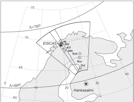
Rov Oul Sod #45 #22 #8 EISCAT Hankasalmi L=60o L=70o #37
Fig. 1. Field-of-view of the Hankasalmi CUTLASS HF radar for ranges in between 400 and 1200 km at the height of 300 km. Dashed lines are 600 and 900 km slant range marks. The outlined sector is the location of beam 5 with the shaded area corresponding to the range bin 16. The solid dot shows the area where ionospheric parameters were measured by the EISCAT incoherent scatter radar. Circles with pluses inside indicate the field-of-view for the Finnish riometers at a height of 90 km. Ellipses with pluses indicate the beam projections at 90 km for the IRIS beams as indicated. Also shown are PACE lines of equal magnetic latitudes of 3 = 60◦and 3 = 70◦.
and Greenwald (1997) concluded that auroral zone echoes occurred more frequently during winter for the direct prop-agation mode, when radio waves reached the ionospheric ir-regularities by means of mildly refracted propagation. The lack of echoes during summer was interpreted as an effect of solar radiation in the sunlit ionosphere smoothing out the plasma gradients and reducing irregularity production. Ruo-honiemi and Greenwald (1997) did not discuss the diurnal variations, but their diagrams show that echoes tend to oc-cur more frequently during late afternoon-midnight-morning hours, although this depends strongly on the season. This might again be indicative of the importance of the irregular-ity production effects.
On the other hand, Milan et al. (1997), by investigating 20-month statistics for the Co-operative UK Twin Located Auroral Sounding System (CUTLASS) HF radars in North-ern Scandinavia, concluded that the electron density in the ionosphere contributes strongly to the echo appearance at a specific range. These authors described changes in the radar wave propagation modes and pointed out that the proper amount of refraction is a very important factor leading to preferential time sectors and radar ranges for echo detection. In addition, they also observed that the low echo occurrence during the winter daytime for short distances is due to a lack of irregularities in the sub-auroral ionosphere. Finally, they confirmed the low echo occurrence during summer. Milan et al. (1997) reported a general decrease in F-region echoes with magnetic activity increase. Ballatore et al. (2001) also noted that there was no clear correlation between the polar cap echo occurrence and the merging electric field intensity,
indicating other factors need to be considered.
To find the reason for the F-region echo appearance, namely the threshold conditions, perhaps one needs to de-termine all of the factors that control the power of echoes when they exist. In the past, only a few attempts have been made in this direction (e.g. Villain et al., 1986; Milan et al., 1999; Fukumoto et al., 2000), mostly due to the difficulty of the measurements of ionospheric parameters within the radar scattering volume. In this study, we combine HF data gath-ered by the CUTLASS Hankasalmi radar with ionospheric measurements performed by the EISCAT incoherent scatter radar and riometer observations along the HF radar beam. We consider an almost 4-day long period in February 1999 and basically employ an approach of Milan et al. (1999).
2 Experiment
In Fig. 1, we show the location of the CUTLASS Hankasalmi HF radar (62.3◦N, 26.6◦E) and its viewing zone between
the ranges of 400 and 1200 km at the height of 300 km. The radar was operated in the high time resolution mode with beam scanning through 16 positions over 1 min. We con-centrate here on observations in beam 5 whose orientation is showed in Fig. 1 by straight lines within the overall view-ing zone. This beam was selected because it overlaps with the region where ionospheric parameters were monitored by the incoherent scatter radar EISCAT (solid circle). The HF radar integration time was around 3 s and the range resolution was 45 km with a starting range of 180 km. The operating
09 Feb 99 12 Feb 99 11 Feb 99 10 Feb 99 Universal Time 00 03 06 09 12 15 18 21 24 a) d) c) b) Range 3000 2400 1800 1200 600 0 Range 3000 2400 1800 1200 600 0 Range 3000 2400 1800 1200 600 0 Range 3000 2400 1800 1200 600 0 1000 m/s 0 m/s -1000 m/s 1000 m/s 0 m/s -1000 m/s 1000 m/s 0 m/s -1000 m/s 1000 m/s 0 m/s -1000 m/s 1000 m/s 0 m/s -1000 m/s
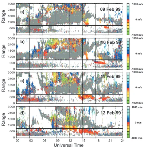
Fig. 2. (a)–(d) Doppler velocity measured by the CUTLASS Hankasalmi radar in beam 5 on 9–12 February 1999. Horizontal solid line at 900 km shows the range corresponding to the area where measurements were made by the EISCAT incoherent scatter radar. The gray color denotes the ground scatter. MLT = UT + 2 h.
frequency was chosen to be 10.0 MHz during nighttime and 12.4 MHz during daytime, to optimize the echo occurrence rate.
The EISCAT UHF radar worked in CP-1K mode with the remote antennas at Kiruna (Sweden) and Sodankyl¨a (Fin-land) being oriented to a common area at a height of 250 km, where additional Doppler velocity measurements were per-formed by the Tromsø receiving antenna along the magnetic flux line. Such an arrangement allowed for tri-static electric field measurements in the area close to bin 16 (slant range of 900 km) of the CUTLASS Hankasalmi radar. In addition to the electric field measurements, the electron density distri-bution with height was derived from the power of the return signals at Tromsø. The altitude resolution for EISCAT den-sity measurements was 22 km for the long pulse method in the F-region, and 3.1 km for the alternate code method in the E- and D-regions. We considered 2-min averaged EISCAT data in this study to have a time resolution as close as possi-ble to the HF radar integration time.
Finally, estimates of non-deviative D-region absorption for HF radio waves were obtained from the 38.2-MHz Imag-ing Riometer for Ionospheric Studies (IRIS) facility located at Kilpisjarvi, Finland (69.1◦N, 20.8◦E) and from Finnish riometer stations at Oulu, Rovaniemi and Sodankyl¨a. The
field-of-view at a height of 90 km for the Finnish riometers and four IRIS beams are indicated by circles and ellipses, re-spectively, with a plus sign indicating the center of the beam. The Finnish stations are located closer to the HF radio wave entry point into the D-region of ionosphere where the major-ity of absorption occurs.
3 Overview of the observational period
We consider the 4-day period of 9–12 February 1999, Figs. 2a–d. The Hankasalmi HF radar observed echoes quite often throughout this interval, although many of the echoes were ground scatter, as indicated in Fig. 2 in gray. Ground scatter is observed when radio waves are refracted to the ground by the ionosphere and reflected back from the ground (for illustrations, see, for example, Villain et al., 1984). Ground scatter was especially strong between 06:00 UT and 18:00 UT, roughly from local sunrise to local sunset (MLT = UT + 2 h). Most of the ground scatter was at slant ranges larger than the EISCAT observation spot (bin 16, range of 900 km), indicated in Fig. 2 by a solid line. Also, short dis-tance meteor-like sporadic echoes were observed most of the time in the evening-midnight-morning sector.
100 200 300 400 Magnetic Disturbance, nT 50 100 150 Electric Field, mV/m -180 -120 -60 0 60 120 180 Azimuth, deg 2 4 6 8 Density, 10 11 m -3
9 Feb 10 Feb 11 Feb 12 Feb 13 Feb
0 12 0 12 0 12 0 12 0
a)
b)
c)
Fig. 3. (a) Horizontal magnetic perturbations at Tromsø, (b) electric field magnitude (solid line) and azimuth (crosses), and (c) electron density at 250 km (solid line) and 110 km (dots). Vertical bars in panels (a) and (b) indicate the times of HF echo occurrence in beam 5, bin 16.
In this study, we are concerned about ionospheric scatter only. For all 4 days, such echoes were observed mostly at large ranges of 2000–3000 km (Figs. 2a–d). It is very likely that these echoes were received through the 1 & 1/2 hop propagation mode, when the radio waves experienced refrac-tion in the F-layer, ground reflecrefrac-tion and propagarefrac-tion to the scatter points with return along the same path. On 9, 10 and 11 February, the F-region densities between ∼10:00 UT and ∼15:00 UT were favorable for maintaining this mode (Milan et al., 1997), as we will show later.
On 9 February, with the electron density decrease after 15:00 UT, near local sunset time, echoes started to be re-ceived at shorter and shorter distances so that between 16:00 and 21:00 UT, the echo band was seen over the EISCAT spot. This general morphology of ionospheric and ground scatter repeated on other days. On 12 February (Fig. 2d), much more ionospheric scatter was detected over the EISCAT spot dur-ing noon hours.
The first 2 days were magnetically quiet, with Kpindices
being around 1, while the other 2 days were moderately dis-turbed with typical Kpindices ranging between 3 and 4
(Cof-fey, 1999). Total horizontal magnetic perturbations (abso-lute value with respect to the background lines for X- and Y-components) at a magnetic station near the EISCAT spot (Tromsø) are presented in Fig. 3a. Very minor perturbations (<100 nT) are seen on 9 and 10 February, and much more significant perturbations (up to 300 nT) in the evening and
midnight MLT sectors on 11 and 12 February (for Tromsø, roughly, MLT = UT + 2 h). In Figs. 3a and c, we indicate, by vertical bars, the times for the ionospheric HF echo appear-ance over the EISCAT spot. A general trend seems to indi-cate that HF echoes occur during times of magnetic distur-bance; however, HF echoes were detected quite often during periods of very low disturbances (10 February, 10:00 UT; 11 February, 06:00–08:00 UT). Also, one can notice an absence of echoes during periods of strongest magnetic disturbances (11 February, 01:00 UT, 14:00 UT; 12 February, 02:00 UT).
Throughout the considered period, the EISCAT radar was operated almost continuously. EISCAT data were available starting from 10:00 UT on 9 February all the way to 16:00 UT on 12 February with an 8-h gap in electric field data on 11 February. The electric field (Fig. 3b) exhibited enhancements during the evening and midnight hours for all days. EISCAT measurements of the ionospheric electron density at 110 km (E-region) and 250 km (F-region) are presented in Fig. 3c. In terms of F-region electron densities, the 9, 10, and 11 Febru-ary events were very much typical, with densities reached around (5 − 7)×1011m−3 in the daytime sunlit ionosphere (sunrise and sunset times are around 06:00 UT and 15:00 UT, respectively). On 12 February, the daytime F-region densi-ties were about 2 times smaller than the previous days. E-region densities were varying sporadically during each day. This is not a surprise since the Sodankyl¨a ionosonde regis-tered sporadic E-layer activity on each day, especially in the
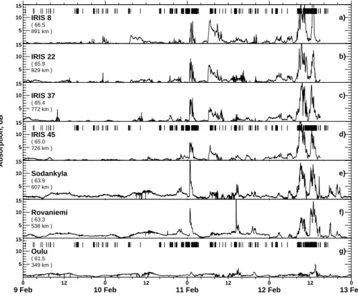
5 10 15 Sodankyla ( 63.9 607 km ) 5 10 15 Rovaniemi ( 63.3 538 km ) 5 10 15 Oulu ( 61.5 349 km ) 5 10 15 IRIS 8 ( 66.5 891 km ) 5 10 15 IRIS 22 ( 65.9 829 km ) 5 10 15 IRIS 37 ( 65.4 772 km ) 5 10 15 IRIS 45 ( 65.0 726 km ) Absorption, dB
9 Feb 10 Feb 11 Feb 12 Feb 13 Feb
0 12 0 12 0 12 0 12 0 a) b) c) d) e) f) g)
Fig. 4. (a)–(g) Variations of D-region absorption at 12 MHz determined by riometers near CUTLASS beam 5, see Fig. 1. Absorption was estimated from original riometer records by applying the f−2dependence, where f is the riometer frequency. Vertical bars in panels (a), (d) and (g) indicate the times of HF echo detection over the EISCAT spot of measurements.
evening and midnight sectors. Clearly, the observed mag-netic perturbations were related to both variations of the elec-tric field magnitude and electron density in the E-layer.
On 10 February, very few ionospheric echoes were ob-served at the EISCAT spot during daytime perhaps partly due to a fairly low electric field, less than 10 mV/m (often even several times smaller). With an electric field increase during evening hours, matched with a decrease in the F-region elec-tron density (due to sunset), echoes started to appear more frequently, especially around magnetic midnight, where F-region densities were favorable for direct propagation mode. Between 17:00 UT and 20:00 UT, a band of E-region echoes was observed at closer ranges of ∼ 700 km.
For 11 February, electric field data were not available for the first 8 h, during which there were some echoes obtained through the direct propagation mode to the EISCAT spot. Later during the day, echoes were observed again for moder-ate values of F-region electron density and electric field.
On 12 February, simple eye inspection shows that HF echo occurrence at the EISCAT spot correlates well with the pe-riod of moderate F-region densities of 2 × 10¹¹m−3, low
E-region densities of less than 1 × 10¹¹m−3and occasion-ally, an enhanced electric field. With the increase of the E-region electron density after 14:00 UT, echoes were observed at ranges ∼ 600 km. Elevation angle measurements indicate that these were E-region echoes.
D-region absorption determined by the riometers near
CUTLASS beam 5 is shown in Fig. 4. Absorption was re-calculated from the original riometer records (at frequencies 30–50 MHz) to the equivalent frequency of f = 12.4 MHz using f−2dependence. Clearly, absorption is almost negli-gible during the first two days and there are some enhance-ments during the other two days, especially in the midnight sector. Also, absorption is larger at higher latitudes, as ex-pected in the auroral zone. One can notice that for some periods, during the considered 4 days (e.g. 10 February, 10:00–16:00 UT) echoes were not detected. During these periods enhanced absorption was observed at low latitudes (e.g. Rovaniemi riometer, Fig. 4f), suggesting that absorp-tion might be a factor in the echo disappearance. On the other hand, one can see that on 12 February, echoes were in abun-dance, even though the absorption was the strongest over the 4-day period. One should also note that there were extended periods when absorption was really small while echoes were not observed.
4 Relationship of echo power and various ionospheric
parameters
From the above review of the period under study, one can conclude that there is no one single factor that dominantly controls the HF echo appearance. In this section, we explore data for those times when HF echoes were observed. We
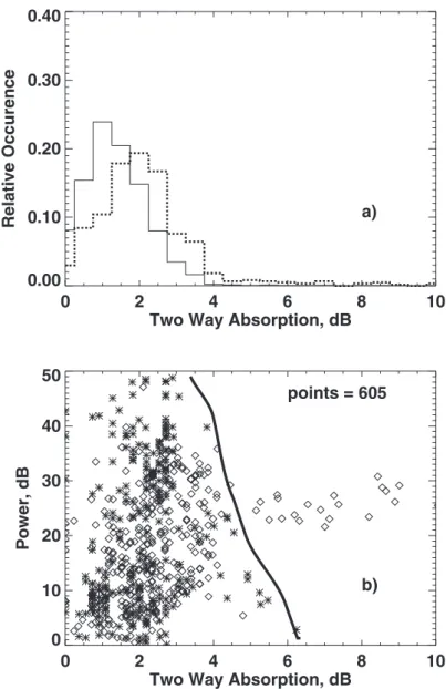
Fig. 5. (a) Histogram of the relative oc-currence of riometer absorption at Oulu for all four days (solid line) and for all times when HF ionospheric echoes were received (dotted line). (b) Scatter plot of HF echo power in bin 16 ver-sus D-region absorption at slant range of ∼ 350 km obtained from the origi-nal riometer records at Oulu, the closest station to the entry point of radar waves into the D-region (605 points). Aster-isks (diamonds) correspond to observa-tions at 10.0 (12.4) MHz.
compare echo power with each of the ionospheric parameters in order to reveal any kind of relationship.
4.1 D-region absorption
Figure 5b shows echo power versus D-region two-way ab-sorption calculated for the radar frequency of 12.4 (10) MHz at the Oulu riometer location. The histograms of occur-rence of riometer absorption (Fig. 5a) for the entire 4 days (solid line) and riometer absorption when ionospheric scat-terers were present during the 4 days (dotted line) indicate that ionospheric scatterers are most likely when the absorp-tion is of the order of 2 dB. One can see that echoes are more intense for small amounts of absorption, less than 3 dB, with the exception of a “separate” cloud of 20 points at ∼ 25 dB. These exceptional data came from observations on 12 Febru-ary, around 13:30 UT (see the spike in absorption on Fig. 4g). The line in Fig. 5b (drawn by hand) determines the limits of the echo power for various amounts of two-way absorption.
This line shows a tendency for the echo power to decrease with absorption, which is expected. However, the majority of observed echoes correspond to small absorption values and the conclusion from this graph is that if F-region echoes oc-cur, the amount of absorption does not substantially reduce their power nor completely absorb the radar waves. Similar conclusions were drawn from the comparison of echo power with absorption at other riometer locations.
4.2 Electron density and radio wave propagation
Previous studies have shown that both E- and F-region densi-ties can be important for the F-region echo appearance (e.g. Milan et al., 1999). Electron density distribution in the iono-sphere controls, first of all, the amount of refraction for ob-servations at a specific range, e.g. Villain et al. (1984). In order to study the role of refraction in our measurements, we temporally assume that F-region irregularities occupy all heights, from the bottom to the top of the F-region. Then the
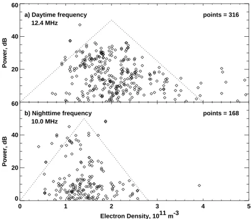
20 40 60 Power, dB points = 316 a) Daytime frequency 12.4 MHz 0 1 2 3 4 5 Electron Density, 1011 m-3 0 20 40 60 Power, dB points = 168 b) Nighttime frequency 10.0 MHz
Fig. 6. Echo power versus electron density at the height of 250 km (a) for the daytime observations at 12.4 MHz (316 points) and (b) for the nighttime observations at 10.0 MHz (168 points). Dotted lines roughly encompass the maximum power observed for each electron density at 250 km.
only concern is an appropriate amount of refraction for the radio waves to reach magnetic flux lines orthogonally within the scattering volume.
In Fig. 6, we present the power of observed echoes ver-sus electron density at the height of 250 km. The available data were split into two sets: the top panel shows daytime observations performed at the radar frequency of 12.4 MHz, while the bottom panel shows similar data for the nighttime observations at the radar frequency of 10.0 MHz . The ten-dency is clear; there is an optimal density that provides the greatest echo power for each radar frequency. These opti-mal values are around 2.0 × 10¹¹m−3for at 12.4 MHz and
1.4 × 10¹¹m−3 at 10.0 MHz. We interpret this result as follows. At densities smaller than the optimal values, the amount of refraction is not enough to meet the orthogonal-ity condition within the expected area of scatter, while for higher electron density over-refraction occurs and again, the orthogonality condition is not met.
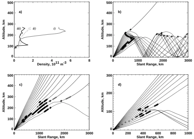
To explore what optimal density means in terms of radio wave propagation for our observations, we made a series of ray tracing modeling for the electron density profiles typi-cally observed by EISCAT during periods of echo registra-tion. We assumed that the density only varies with altitude, since two-dimensional measurements of the profiles are not available in the CP1 mode. By the identification of com-mon radar features predicted by the ray tracing, we believe
this approach is a valid first order approximation. In Fig. 7a, we show three 10-min electron density profiles, as measured by EISCAT at 12:30 UT on 10 February (case (i)), and at 12:30 UT (case (ii)) and 14:30 UT (case (iii)) on 12 Febru-ary. In Figs. 7b–d, we show the slant ranges and altitudes of expected backscatter (with aspect angles within ±1◦range)
by crosses along specific rays where the rays correspond to elevation angles of 6◦–30◦in 2◦steps.
In Fig. 7b, we show that for electron densities typical for daytime observations on several days, there are no chances to receive direct F-region echoes at ∼ 900 km, but there are opportunities to receive 1 & 1/2 hop signals at ∼ 2500 km. Also, reception of ground scatter is very likely from 1200– 2800 km. Ionospheric echoes are expected to come from the altitudes of 190–250 km with elevation angles of 20◦–30◦. These values of elevation angles are in reasonable agreement with radar measurements. This diagram also predicts that echoes (from both E- and bottom F-regions) can be obtained from short distances, but they were not detected according to Fig. 2b, except for sporadic traces of echoes at near ranges of 300–600 km. We believe that E-region echo absence is related to the low electric field observed at this time.
Figure 7c shows how propagation is affected due to a sub-stantially decreased F-region density, as was typical during the daytime of 12 February. One can see no 1 & 1/2 hop propagation mode here. After 14:00 UT, the E-region
elec-0 2 4 6 8 Density, 1011 m-3 0 100 200 300 400 500 Altitude, km i) ii) iii) a) 0 1000 2000 3000 Slant Range, km 0 100 200 300 400 500 Altitude, km b) 0 1000 2000 3000 Slant Range, km 0 100 200 300 400 500 Altitude, km c) 0 200 400 600 800 1000 Slant Range, km 0 100 200 300 Altitude, km d)
Fig. 7. (a) The electron density distribution in the ionosphere used in ray tracings (b)–(d) and possible ray paths for 12.4 MHz observations from Hankasalmi for (b) 10 February 12:30 UT, using profile i), (c) 12 February 12:30 UT, using profile ii), and (d) 12 February 14:30 UT, using profile iii). Crosses indicate ranges where the ray is within ±1◦of orthogonality to the magnetic field.
tron density was enhanced, which caused the rays to reach orthogonality only in at E-region altitude and at much shorter ranges, as depicted in Fig. 7d. Thus, ray tracing supports our conclusions on the propagation modes that were in effect during our measurements.
Another way the electron density distribution can affect the appearance of F-region irregularities is through slowing down the gradient-drift (GD) instability responsible for the irregularity excitation. This happens due to shorting out the polarization electric field in growing GD modes (Vickrey and Kelley, 1982; Chaturvedi et al., 1994). We will explore this effect in the next sub-section, since it is closely related to the intensity of the electric field in the ionosphere.
4.3 Electric field intensity
The existence of ionospheric irregularities of appropriate scale size ultimately determines the appearance of auroral echoes; without the irregularities no return echo could be de-tected. Unfortunately, not much is known about the proper-ties of F-region irregulariproper-ties of decameter scale (Fejer and Kelley, 1980; Hanuise, 1983; Tsunoda, 1988). In the auro-ral zone, the most likely mechanism of F-region irregularity formation is the gradient-drift instability. The positive con-tribution to the growth rate of the GD instability is deter-mined by the electric field magnitude, the scale of the
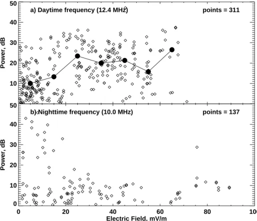
back-ground gradient and their mutual orientation (Keskinen and Ossakow, 1982). Damping of the GD waves is determined by the diffusion (dependent on the temperatures and collision frequencies of charged particles). As mentioned above, dif-fusion can be enhanced in the presence of highly conducting E-layer (Vickrey and Kelley, 1982). According to Vickrey and Kelley (1982), the effect is determined by the param-eter ζ = 1 − M−1, where M = 1 + 6Fp/6pE and 6pE and 6pF are the height integrated Pedersen conductances of the E-and F-layers, respectively. For a poorly conducting E-layer, 6pE →0, M → ∞ and ζ → 1. For a highly conducting E-layer, M → 1 and ζ → 0 and the growth rate of the GD in-stability is greatly decreased. In this section, we explore the role of both these factors in observations of F-region echoes. Figure 8 is a scatter plot of echo power versus electric field magnitude separated once again into daytime and nighttime events. There is a significant data spread here; however, dur-ing the daytime, points seem to show a power increase, as indicated by the shaded circles which represent the average power in each 10 mV/m electric field bin. Overall, one can say that a stronger electric field is preferred. For the night-time, no such trend is seen. However, for the night-time fre-quency, there does appear to be a limit in the electric field of about 20 mV/m above which the power does not exceed 20 dB. Indeed, some echoes observed at electric fields as high as 80 mV/m were of low intensity.
10 20 30 40 50 Power, dB points = 311 a) Daytime frequency (12.4 MHz) 0 20 40 60 80 100 Electric Field, mV/m 0 10 20 30 40 50 Power, dB points = 137 b) Nighttime frequency (10.0 MHz)
Fig. 8. Scatter plot of echo power versus electric field magnitude for all echoes observed over 4 days (a) for daytime observations at 12.4 MHz (311 points) and (b) for nighttime observations at 10.0 MHz (137 points). Shaded circles in (a) indicate the average power in the associated 10 mV/m electric field bin.
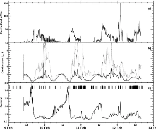
In Fig. 9, we explore the effect of a conducting E-layer on the echo appearance. We plot here the height-integrated con-ductances of the E- and F-layers and the parameter M for the times when EISCAT density measurements are available. We represented the E-layer arbitrary as being contained between 90 and 140 km, with the F-layer being spread over altitudes above 140 km, similar to Milan et al. (1999). We also indi-cate by vertical bars in Fig. 9c the times for the echo appear-ance over the EISCAT spot. The general impression from Fig. 9 is that echoes are mostly observed during the times of low values of the M factor. Contrary to expectation, every time M was enhanced at noon, very few echoes were seen. One should note that periods of high M values typically also coincide with periods of low electric field, so the judgment on the importance of the effect is difficult to ascertain. For example, on 11 February, the echoes were seldom between 08:00 UT and 13:00 UT, even though the M value was en-hanced and the electric field was about 10 mV/m or so. On the other hand, on 12 February, at ∼02:00 UT, echoes were observed, as predicted, when the M values were enhanced, perhaps due to a simultaneously enhanced electric field.
One important feature of the data presented in Fig. 9 worth mentioning is that the observations right at the end of the pe-riod on 12 February at 14:00–15:00 UT show M values to be unusually low, while the electric field was strong, but no echoes were observed. To clarify this point, we present data
for 12 February, 10:00–16:00 UT in Fig. 10 with better time resolution than data in Fig. 9. One can see the effect easily as the value of M approaches 1; the instability is inhibited. However, this is not the likely reason for the lack of F-region echoes at this time. As we discussed in Sect. 4.2, echo disap-pearance at this time is very likely due to enhanced density in the lower portion of the ionosphere, so that HF radar waves are refracted to smaller heights and closer ranges (Fig. 7d). Another similar event is around 11:40 UT on this day.
On the other hand, looking at Fig. 10 and Fig. 7c, one can notice that short-lived echo disappearance is not always re-lated to propagation effects. For example, around 13:00 UT, there was no significant redistribution of electron density (no change in conductance), but echoes disappeared, perhaps due to the decrease in electric field magnitude.
5 Discussion
Over the last decade, statistics for various parameters of F-region HF coherent echoes have been reported, including power, spectral width and velocity (Milan et al., 1997; Milan and Lester, 1998; Huber, 1999; Fukumoto et al., 1999, 2000; Hosokawa et al., 2001, 2002). However, not much attention has been paid to a fundamental question on the major fac-tor(s) controlling the appearance of such echoes. Certainly,
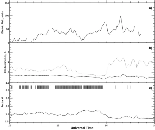
50 100 150 Electric Field, mV/m 2 4 6 8 10 Conductance, Σp , S 1.0 1.5 2.0 2.5 3.0 3.5 Factor M
9 Feb 10 Feb 11 Feb 12 Feb 13 Feb
0 12 0 12 0 12 0 12 0
a)
b)
c)
Fig. 9. Temporal variations of (a) the electric field, (b) the height-integrated Pedersen conductances in the F- and E-regions (solid line and dots, respectively), (c) the parameter M = 1 + 6pF/6Ep influencing the growth rate of the F-region gradient-drift instability in the presence of conducting E-region and HF echo occurrence over the EISCAT spot (vertical bars).
it is not easy to address this question without reliable knowl-edge of irregularity availability and of plasma parameters all along the propagation path of the HF radar wave, including, of course, the scattering volume. It is important to realize that at HF, several propagation modes are important, so that an assessment of various factors certainly should take this circumstance into account.
In this study, we consider the simplest case when F-region echoes are received through the direct F-region propagation mode. In this case, radio waves reach F-region irregulari-ties through the appropriate amount of refraction (this mode is also called 1/2F mode, Milan et al., 1997). But even for this simple situation, we had a very limited data set to work with. Namely, we had measurements of electron densities at the scattering volume and extrapolated these measurements along the HF radar beam. One should also bear in mind that the areas of EISCAT and CUTLASS effective collecting vol-umes are quite different for each instrument. EISCAT mea-sures parameters in an area with a diameter of ∼ 3 km at the height of 250 km, while the effective area for the CUTLASS radar has dimensions of ∼ 45 km × 150 km. No information on irregularity heights was available. Without knowing much about the thickness of the irregularity layer for the HF mea-surements (is it several kilometers or hundred kilometers?), the conclusions drawn from the ray tracing are not decisive. The effect of the irregularity filling the coherent radar beam
has been studied by Walker et al. (1987).
For the event under consideration, we found that echo de-tection at the point of EISCAT observations (geomagnetic latitude of ∼ 66.5◦) is strongly determined by the propaga-tion condipropaga-tions. The electron density distribupropaga-tion in the iono-sphere must be appropriate to support radio wave propaga-tion exactly to the expected area of joint observapropaga-tions, as in Fig. 7c.
Most of the echoes at the EISCAT observational area tended to occur during evening and midnight hours, the pref-erential period for Hankasalmi echoes at these latitudes (Mi-lan et al., 1997). Echoes occurred for electron densities in between 1.0 × 10¹¹m−3and 4 × 10¹¹m−3, which is exactly what is needed for radio wave focusing to the F-layer heights, according to the ray tracing analysis. The derived densities are consistent with the finding of Milan et al. (1997) that echoes typically occur for an F-layer critical frequency of 4 MHz.
One should say that during daytime/early evening hours in February 1999 stronger densities in the F-layer are usually achieved (according to the EISCAT measurements for 9, 10 and 11 February and according to the Sodankyl¨a ionosonde statistics, see Milan et al. (1997), Fig. 7). Hence, the direct mode for F-region echoes should occur, if ever, at shorter dis-tances. Hankasalmi echo occurrence rates published by Mi-lan et al. (1997) do not have enough spatial resolution to see
50 100 150 Electric Field, mV/m 2 4 6 8 Conductance, Σp , S 1.0 1.5 2.0 2.5 3.0 3.5 Factor M 10 12 14 16 Universal Time a) b) c)
Fig. 10. The same as in Fig. 9, but for 12 February 1999 observations between 10:00 and 16:00 UT.
the effect, while Hosokawa et al. (2001) did not consider very low latitudes. Recent echo occurrence analysis performed by D. Andr´e (results are not published) confirms that maxi-mum of echo occurrence for February 1999 is located at 2◦–
3◦ lower than normal latitudes, in agreement with
expecta-tions. Our observations for 9, 10, and 11 February are also in agreement with this expectation. On 12 February, echoes were observed in the noon sector, but as we demonstrated, the densities were ∼ 2 times smaller during this day.
One would expect another desirable effect with density increase, namely a better chance to obtain echo detection through the 1 & 1/2 propagation mode, since in this case, strong bending is more likely through refraction. Milan et al. (1997) clearly demonstrated that Hankasalmi daytime echoes are typically cusp/cleft echoes obtained through this mode, and other reports (e.g. Ruohoniemi and Greenwald, 1997; Hosokawa et al., 2001) support this conclusion.
One should mention that Hosokawa et al. (2001) found quite a few afternoon/evening echoes being produced at the poleward edge of the mid-latitude ionospheric trough. As we mentioned in Sect. 3, indeed echoes started to be observed more frequently right after the local sunset for the F-region, so the horizontal plasma gradient associated with the trough might have contributed well to the preferential irregularity formation during these hours. In addition, Hosokawa et al. (2001) did find a second morning peak in echo occurrence for the Canadian radars, but not for the Hankasalmi radar. In our event, quite a few echoes were observed during
morn-ing hours on 10 and 11 February and perhaps on 9 Febru-ary (EISCAT measurements are not available here, but So-dankyl¨a ionosonde data support this conclusion) prior to lo-cal sunrise. One can conclude that F-region echoes at the EISCAT spot for February can be related to the trough. For certain, echoes are seen when the ionosphere experiences a transition from the daytime to the nighttime configuration in the evening sector and from the nighttime to the daytime in the morning sector.
Our conclusion of the primary role of refraction as a factor for the HF echo appearance refers to one specific point in the Hankasalmi radar field-of-view (FoV). It cannot be simply extrapolated to other areas within this radar FoV, not to say anything about other SuperDARN radars. Besides refraction, the issue here is whether strong F-region irregularities exist at all ionospheric heights accessible to radar waves. This is especially important for observations within the polar cap, where the background density is not strong enough to support refraction as it can in the auroral zone. Polar cap patches of F-region background ionization are important in two ways: they provide enhanced refraction and, on the other hand, the gradients at their edges are the primary areas for the exci-tation of the GD instability (Tsunoda, 1988). These clouds are certainly limited in their horizontal extent and height. So for the polar cap echoes the propagation conditions should be matched with the irregularity production conditions.
The prime importance of proper refraction conditions for echo appearance does not mean that other factors are not
im-portant. First of all, with respect to the D-region absorption, we should mention that the events under consideration were, by chance, for quiet and moderately disturbed days. The ab-sorption was very small at the range (∼ 300 km) where the rays that intersect the F-region at ∼ 900 km were passing through the D-region. Stronger absorption was detected at some larger ranges, which might affect scatter at ranges be-yond 900 km, although this assessment is complicated due to the presence of ground scatter at these ranges. We would ex-pect more significant importance of D-region absorption dur-ing more disturbed days when the region of strong particle precipitation is shifted equatorward. It is well documented now that HF radar echoes quickly disappear at the expansive phase of a substorm developing in the local time sector of radar measurements (e.g. Voronkov et al., 1999).
The irregularity production factors are also important. For the considered events, the IMF Bz component was mostly
negative, so that one would expect mostly strong electric fields in the auroral zone, and the EISCAT measurements in-deed show E fields in excess of the 5–10 mV/m needed for the excitation of the GD instability. The daytime data pre-sented in Fig. 8 indicate that echo power generally increases with electric field. This conclusion is consistent with the sta-tistical analysis of the echo power-Doppler velocity relation-ship performed by Fukumoto et al. (1999, 2000). These au-thors found that the power of echoes increases with the l-o-s velocity, clearly during daytime, and in more complicated fashion in the midnight sector. This is similar to our results, if one assumes that the l-o-s velocity increases because of elec-tric field enhancement (power variations with the flow angle are not expected for the F-region echoes, though analysis of this effect has not been done yet). One would expect the den-sity fluctuation level increase with the electric field, since GD instability is strongly dependent on the electric field magni-tude (Tsunoda, 1988).
Our analysis shows that besides a strong electric field, the conductance of the E-region must be taken into account when the irregularity production is considered; this conclusion is similar to one of Milan et al. (1999). For example, on 11 February, between 16:00 and 18:00 UT, the propagation con-ditions were satisfactory, Ne = 2 × 10¹¹m−3, the electric
field was of reasonable intensity, 20 mV/m, and as a conse-quence of reasonably small M values, echoes were not seen over the EISCAT spot. However, the situation was not al-ways clear. Contrary to prediction, we showed that echoes were not always observed when M factor values were large. Several other effects can explain the echo absence over the EISCAT spot. One of these is that propagation conditions might have been such that one would need irregularities to be intense below 200 km. It well might be that irregularities simply were not generated at these heights. It is expected that the GD instability is efficient at the edges of plasma clouds in the F-region, and it might be that ionospheric gra-dients were not strong enough to generate the irregularities, although with the current experiment, the horizontal gradient could not be measured. Further studies should be carried out to ascertain the effects of horizontal gradients on the
produc-tion of F-region irregularities.
6 Conclusions
In this study, we attempted to evaluate the factors influenc-ing the F-region echo appearance at a specific spot in the high latitude ionosphere. The monitored area was conveniently lo-cated for a direct HF propagation mode. A 4-day period was considered with 2 relatively quiet days and 2 moderately dis-turbed days. Overall, significant amounts of echoes were ob-served. We found that D-region absorption is a minor factor for the echo detection. Often absorption just decreased the power of the signals. We also demonstrated that echoes were more intense for a stronger electric field, though often, they occurred for a fairly low electric field of ∼ 10 mV/m. The most significant factor that controls echo appearance was the electron density distribution in the ionosphere, both in the E-and F-regions. F-region density controls radio wave propa-gation/focusing to the test spot and the density needs to be in between 0.5 × 10¹¹m−3and 4 × 10¹¹m−3. E-region density, besides supporting the propagation mode, may perhaps influ-ence the wave electric field of F-region irregularities, so that in the case of a very dense E-region, the instability is slowed down or even prevented by the enhanced conductance.
Acknowledgements. CUTLASS Finland radar is supported by
PPARC, the Swedish Institute for Space Physics, Uppsala, and the Finnish Meteorological Institute. EISCAT is an international facil-ity supported by Finland, France, Germany, Japan, Norway, Swe-den and the UK. Data of the Sodankyl¨a ionosonde and Finnish riometers are from the Sodankyl¨a Geophysical Observatory. Ad-ditional riometer data originated from the Imaging Riometer for Ionospheric Studies (IRIS), operated by the Department of Com-munications Systems at Lancaster University (UK), funded by the Particle Physics and Astronomy Research Council (PPARC) in collaboration with the Sodankyl¨a Geophysical Observatory. The geomagnetic data are from the Tromsø Geophysical Observatory (Nordlysobservatoriet), University of Tromsø, Norway. A.V.K. ac-knowledges the Solar-Terrestrial Environment Laboratory of the Nagoya University for funding during his stay in Japan. The work was also supported by an NSERC grant (Canada) to A.V.K. The authors are grateful to K. Schlegel and R. Woodman for helpful dis-cussions.
The Editor in chief thanks two referees for their help in evaluat-ing this paper.
References
Ballatore, P., Villain, J.-P., Vilmer, N., and Pick, M.: The influence of the interplanetary medium on SuperDARN radar scattering oc-currence, Ann. Geophysicae, 18, 1576–1583, 2001.
Chaturvedi, P. K., Keskinen, M. J., Ossakow, S. L., and Fedder, J. A.: Effects of field line mapping on the gradient-drift insta-bility in the coupled E- and F-region high-latitude ionosphere, Radio Sci., 29, 317–335, 1994.
Coffey, H.: Geomagnetic and solar data, J. Geophys. Res., 104, 22 819–22 820, 1999.
Fejer, B. G. and Kelley, M. C.: Ionospheric irregularities, Rev. Geo-phys., 18, 401–454, 1980.
Fukumoto, M., Nishitani, N., Ogawa, T., Sato, N., Yamagishi, H., and Yukimatu, A. S.: Statistical analysis of echo power, Doppler velocity and spectral width obtained with the Syowa South HF radar, Adv. Polar Upper Atmos. Res., 13, 37–47, 1999.
Fukumoto, M., Nishitani, N., Ogawa, T., Sato, N., Yamagishi, H., and Yukimatu, A. S.: Statistical study of Doppler velocity and echo power around 75◦magnetic latitude with the Syowa East HF radar, Adv. Polar Upper Atmos. Res., 14, 93–102, 2000. Greenwald, R. A., Baker, K. B., Dudeney, J. R., et al.:
DARN/SuperDARN: A global view of the dynamics of high-latitude convection, Space Sci. Rev., 71, 761–796, 1995. Hanuise, C.: High-latitude ionospheric irregularities: a review of
recent results, Radio Sci., 18, 1093–1121, 1983.
Hosokawa, K., Iyemori, T., Yukimatu, A. S., and Sato, N.: Source of field aligned irregularities in the subauroral F-region as ob-served by the SuperDARN radars, J. Geophys. Res., 106, 24 713– 24 731, 2001.
Hosokawa, K., Woodfield, E. E., Lester, M., Milan, S. E., Sato, N., Yukimatu, A. S., and Iyemori, T.: Statistical characteristics of spectral width as observed by the conjugate SuperDARN radars, Ann. Geophysicae, 20, 1213, 2002.
Huber, M.: HF radar echo statistics and spectral studies using Su-perDARN, M.Sc. Thesis, University of Saskatchewan, Saska-toon, Canada, 1999.
Keskinen, M. J. and Ossakow, S. L.: Nonlinear evolution of plasma enhancements in the auroral ionosphere. 1. Long wavelength ir-regularities, J. Geophys. Res., 87, 144–150, 1982.
Milan, S. E., Yeoman, T. K., Lester, M., Thomas, E. C., and Jones, T. B.: Initial backscatter occurrence statistics from the CUT-LASS HF radars, Ann. Geophysicae, 15, 703–718, 1997. Milan, S. E. and Lester, M.: Simultaneous observations at
differ-ent altitudes of ionospheric backscatter in the eastward electrojet, Ann. Geophysicae, 16, 55–68, 1998.
Milan, S. E., Davies, J. A., and Lester, M.: Coherent HF radar backscatter characteristics associated with auroral forms identi-fied by incoherent radar techniques: A comparison of CUTLASS and EISCAT observations, J. Geophys. Res., 104, 22 591–22 604, 1999.
Ruohoniemi, J. M. and Baker, K. B. : Large-scale imaging of high-latitude convection with Super Dual Auroral Radar Network HF radar observations, J. Geophys. Res., 103, 20 797–20 811, 1998. Ruohoniemi, J. M. and Greenwald, R. A.: Rates of scattering occur-rence in routine HF radar observations during solar cycle maxi-mum, Radio Sci., 32, N3, 1051–1070, 1997.
Tsunoda, R. T.: High latitude irregularities: A review and synthesis, Rev. Geophys., 26, 719–760, 1988.
Villain, J.-P., Greenwald, R. A., and Vickrey, J. F.: HF ray trac-ing at high latitudes ustrac-ing measured meridional electron density distribution, Radio Sci., 19, 359–374, 1984.
Villain, J.-P., Beghin, C., and Hanuise, C.: ARCAD3-SAFARI co-ordinated study of auroral and polar F-region ionospheric irregu-larities, Ann. Geophysicae, 4, 61–73, 1986.
Vickrey, J. F. and Kelley, J. D.: The effects of a conducting E-layer on classical F-region cross-field plasma diffusion, J. Geophys. Res., 87, 4461–4468, 1982.
Voronkov, I., Friedrich, E., and Samson, J. C.: Dynamics of the substorm growth phase as observed using CANOPUS and Su-perDARN instruments, J. Geophys. Res., 104, 28 491–28 505, 1999.
Walker, A. D. M., Greenwald, R. A., and Baker, K. B.: Determi-nation of the fluctuation level of ionospheric irregularities from radar backscatter measurements, Radio Sci., 22, 689–705, 1987.