HAL Id: hal-00267762
https://hal.archives-ouvertes.fr/hal-00267762
Submitted on 28 Mar 2008
HAL is a multi-disciplinary open access archive for the deposit and dissemination of sci-entific research documents, whether they are pub-lished or not. The documents may come from teaching and research institutions in France or
L’archive ouverte pluridisciplinaire HAL, est destinée au dépôt et à la diffusion de documents scientifiques de niveau recherche, publiés ou non, émanant des établissements d’enseignement et de recherche français ou étrangers, des laboratoires
How long can excess pollution persist? The
non-cooperative case
Pierre-Yves Hénin, Katheline Schubert
To cite this version:
Pierre-Yves Hénin, Katheline Schubert. How long can excess pollution persist? The non-cooperative case. Resource and Energy Economics, Elsevier, 2008, 30 (2), pp.277-293. �10.1016/j.reseneeco.2007.04.001�. �hal-00267762�
How long can excess pollution persist? The non-cooperative
case
Pierre-Yves Hénin
Université Paris 1 Panthéon–Sorbonne.
Katheline Schubert y
Université Paris 1 Panthéon–Sorbonne.
March 2007
Abstract
This paper describes a world composed of two (groups of) countries, which derive their utility from a polluting activity and from the enjoyment of a common environmental quality. The initial situation is both suboptimal and unsustainable: pollution leads to a continuous deterioration of environmental quality. The two countries have heterogeneous preferences for the environment, which are private knowledge. This prevents the adoption of abatement policies negotiated between the two countries, because each one has a strong incentive to announce in every negotiation an arbitrarily low preference for the environment. The two countries then engage in a war of attrition, each of them postponing abatement policies, in the hope that the other will concede …rst and abate more. We study for how long the adjustment is postponed, according to initial conditions, the greenness of the greenest country, the possible range of preferences and the rates of discount and natural regeneration.
keywords: war of attrition, environmental negotiations, climate change JEL classi…cation: C72, Q20
Corresponding author. Address: Centre d’Economie de la Sorbonne, 106–112 bd. de l’Hôpital, 75647 Paris Cedex 13, France. E-mail: [email protected]
yWe thank Martine Carré, Jean-François Jacques and Larry Karp for their helpful suggestions, criticisms and
1
Introduction
International negotiations about environmental public goods are often disappointing, with ad-vances closely followed by backward steps. In the …eld of climate change for example, recent events –particularly President Bush’s rejection of the Kyoto Protocol– show that it is easier to postpone measures aimed at reducing greenhouse gas emissions than to reach an agreement on the sharing of e¤orts to reduce these emissions. We now have good reasons to expect that size-able international pollution abatement will be further delayed, thus raising the question: how long can excess pollution persist?
The literature has tackled the question of international negotiations about environmental public goods in two ways.
The …rst approach analyses the problem in a cooperative framework and de…nes the mech-anisms able to sustain cooperation (see for example Chander and Tulkens, 1992, 1995). But recent experiences in the …eld of climate change argue in favor of non-cooperative approaches. Moreover, we are interested in this paper in the mechanisms that allow non-cooperation to persist, thus preventing the emergence of stabilization.
The second approach consists in looking at the formation of environmental agreements from the point of view of non-cooperative game theory (see for example Barrett, 1994, 1998, Carraro and Siniscalco, 1993, Hoel, 1992). Most theoretical papers in this strand of the literature retain an assumption of homogeneous countries, and focus on the size of the coalitions that can emerge. Our intention is to study the behaviour of heterogeneous countries in a two countries set-up, thus eliminating the question of formation of coalitions.
We describe a world composed of two groups of countries, which derive their utility from a polluting activity but also from the enjoyment of a common environmental quality. The initial situation is commonly known as both suboptimal and unsustainable in the sense that global pollution is excessive and leads to a continuous deterioration of environmental quality over time. The main assumption is that the two groups of countries have di¤erent preferences as far as environmental quality is concerned. Apart from their divergence in the valuation of
environmental assets, the two groups of countries are identical and emit the same amount of pollution in the business-as-usual pre-stabilization situation.
As far as climate change is concerned, these two groups of countries can be seen as the Euro-pean countries on the one hand and the United States on the other hand. Their environmental consciousness is di¤erent, and so is their evaluation of the reality of the climate change problem. Moreover, they do not agree on the means that must be brought into play to tackle it. While European countries favor the Kyoto Protocol, the United States is skeptical and seems to rely on technical progress to deal with this problem, without the need of additional initiatives that could jeopardize U.S. growth.
The preference for the environment cannot be reduced to a subjective environmental con-sciousness. It also re‡ects the marginal damage caused by the worsening of environmental quality or, equivalently, the marginal bene…t of an improvement in environmental quality, and countries di¤er in this respect. It is di¢ cult for either group of countries1 to know the level of preference
for the environment of the other, since this preference is a mix of subjective environmental con-sciousness and of objective marginal damage. In addition, each country behaves strategically and is tempted to announce biased preferences in negotiations in order to manipulate information.
The environmental preference is therefore private knowledge. This asymmetry of information prevents the emergence of a negotiated solution, because each country has a strong incentive to announce an arbitrarily low preference for the environment. The two countries then engage in a war of attrition, each of them postponing the implementation of measures intended to reduce pollution with the hope that the other one will concede …rst.
War of attrition models have been applied to various issues, such as labor strikes, biological competition, industrial organization and, in the political economy …eld, …scal stabilization. Bac (1996) underlines their relevance in the case of environmental questions. In this paper we adopt a framework closely related to war of attrition models applied to …scal stabilization (Alesina and Drazen, 1991, Casella and Eichengreen, 1996, Carré, 2000), because our case has in common
1
In the following, we will content ourselves with speaking of two countries instead of two groups of countries, for ease of reference.
with these models its stock-‡ow structure, the stock being a public good and the ‡ow a private advantage. Compared to these models, the game we consider in this paper nevertheless has several distinctive features.
First, in the …scal stabilization problem, stabilization can always be postponed; it is not the case in our model where if nothing is done in …nite time, the environmental capital reaches a minimal threshold that cannot be passed. Carré (2000), building on Alesina and Drazen’s model, introduces an exogenous deadline such that if …scal stabilization has not occurred before this date a penalty is paid by all players. Our model cannot be reduced to this framework, because it is impossible here for the agents to decide to pass beyond the deadline.
Secondly, due to the lack of a supra-national authority, the burden of stabilization cannot be shared, even unequally, between the two players2. We consider that one of the countries, the loser, can decide unilaterally to try to stabilize environmental quality. We also show that if nothing is done to stabilize environmental quality before a certain limit date, stabilization requires that both countries reduce pollution. There are then two games: a …rst one where environmental conditions are such that one country can stabilize alone, and a second one where environmental conditions are so deteriorated that both countries must reduce pollution in order to achieve stabilization.
The paper is organized as follows. Section 2 sets the framework and the basic assumptions of the model. In Section 3, information is assumed to be asymmetric. Considering the case where an immediate stabilization would occur under perfect information, we study how long the adjustment will be postponed, and the in‡uence of the parameters that characterize each country. We show that there exists a critical parameter of preference for the environment, which depends on initial conditions, on the possible range of preferences and on the rates of discount and natural regeneration. If the parameter of preference of the greenest country is greater than this critical value, the optimal stabilization date is, loosely speaking, not too far, and this country will stabilize environmental quality alone. If the environmental parameter is less than
2
The absence of any supra-national authority provides a strong rationale for representing the global environ-mental problem as a war of attrition. This rationale is not as strong in the case of …scal stabilization issues.
the critical value, stabilization will be late and both countries will have to reduce pollution. In that case, if the discount rate is high enough, an accumulation of concessions at the limit date by which the natural capital reaches its minimal threshold occurs. If the discount rate is even higher, a jump in the concession function can appear. Section 4 concludes and discusses possible extensions.
2
The model
2.1 The general framework
Two countries derive their utility from consumption and from the enjoyment of a common environmental quality. Emissions of pollution of country i; pi(t); are strictly proportional to
economic activity and hence to consumption. From an initial level q0; global environmental
quality q(t) is deteriorated by the polluting activity of both countries but regenerates at a constant rate > 0. Its law of motion is then
_
q(t) = q(t) (p1(t) + p2(t)) : (1)
Environmental quality is de…ned as the di¤erence between the current level of natural capital and the minimal level necessary to support human life, below which natural capital cannot fall. The constraint q(t) 0 must then be satis…ed.
The instantaneous utility of country i; ui(t); is supposed linear in its two arguments, country
i’s pollution and global environmental quality3:
ui(t) = pi(t) + iq(t) i = 1; 2; (2)
where i is the “preference for the environment” of country i and characterizes the “greenness”
of preferences. The intertemporal welfare of country i is the sum of the instantaneous utilities discounted at a constant rate > 0; supposed identical for the two countries.
3
This linearity assumption is usual in the war of attrition literature because it enables a complete analytical characterization of the solution. But it has obvious drawbacks, mainly the fact that utility remains …nite as environmental quality approaches zero, and so nothing prevents the optimal choice of a zero environmental quality. But history reminds us that such a choice can actually exist, through, for example, the famous case of Easter Island.
The business-as-usual pollution level is assumed to be constant and identical for the two countries4, and is denoted by p > 0. Total pollution is then 2p in BAU. Thus, the preference parameter is the only feature that distinguishes one country from the other in the BAU situation. In BAU, the environmental quality level at date t is given by:
qB A U(t) = q0e t+
2p
1 e t : (3)
We focus on the case of excessive initial pollution: we suppose p > 2q0; so that environmental
quality deteriorates if nothing is done to reduce pollution. Thus the world economy follows, in the BAU situation, an unsustainable pollution path.
In order to stabilize environmental quality at time t, global pollution must be reduced to the level P (t) such that _q(t) = 0, which requires that it becomes just equal to natural regeneration:
P (t) = qB A U(t): (4)
P (t) is the sustainable pollution level. Obviously, the global e¤ort required to stabilize environ-mental quality, equal to 2p P (t) at time t; is all the larger since stabilization occurs at a later date.
Within the non-cooperative framework considered in this paper, a solution to the environ-mental problem consists in …nding i) the country that makes the …rst e¤ort of stabilization, and ii) the date at which this occurs5.
2.2 The limit dates
We de…ne a …rst limit date Tmas the last date at which one country is able to stabilize
environ-mental quality by itself. At Tm; the required reduction of total pollution (2p P (Tm)) equals the
4
The assumption of exogenous, constant and identical BAU emissions for the two countries is admittedly unrealistic, but we have made it in order to avoid the mix of two di¤erent problems: (1) the determination of the optimal path of pollution of each country before they become aware of the necessity to stabilize environmental quality (the “historical” or BAU behavior of each country); and (2) the behavior of each country after it realizes the necessity to stabilize environmental quality: will it stabilize and, if yes, when? In other words, this assumption is necessary to reduce the problem to one dimension: the choice of one date.
5
Notice that our purpose is di¤erent from that of Dockner and Van Long (1993), who study, in the linear– quadratic case, an optimal control of pollution problem with perfect information. We do not try to answer the question of the optimal reduction of pollution of each country at each date, in order to concentrate on the war of attrition problem.
total pollution by one country (p). Thus the country that reduces emissions …rst (the loser, to follow the terminology usual in war of attrition models) at time Tm must reduce its pollution to
zero in order to stabilize environmental quality, while the other country (the winner ) continues to pollute p. Date Tm is then de…ned by
P (Tm) = p = qB A U(Tm) , qB A U(Tm) =
p
, q0e Tm+
2p
1 e Tm = p;
from which we obtain
Tm =
1
ln p
2p q0
: (5)
This date is strictly positive if and only if p < q0: In the opposite case, a single country cannot
stabilize. So we suppose this condition ful…lled in the rest of the paper . We then have, in the initial situation:
Assumption 1 2q0 < p < q0: The initial environmental quality q0 can sustain one unrestricted
polluting country, but not two, i.e. global pollution emissions greater than p but less than 2p:
The higher the initial pollution p; the closer the limit date Tm, and the higher the initial
environmental quality q0; the later Tm.
If none of the two countries decides to stabilize before date Tm, it becomes too late for one
country to stabilize by itself. After Tm; if the greenest country decides to concede at a date eT ;
it must cut its pollution to zero, but that will not be enough, and stabilization of environmental quality will only take place if the other country also reduces its pollution, to a level just equal to the natural regeneration capacity. The problem is then to …nd when the winner will accept to bear its part of the burden of adjustment, actually smaller than the part of the loser: as soon as the loser concedes (that is to say at eT ), later, or never?
Let us suppose that the loser decides to reduce its pollution to zero at eT > Tm: From eT
to the date T at which the winner decides to bear its part of the burden, environmentale quality evolves according to the following equation:
_
and so environmental quality is given by
q(t) = qB A U( eT )e (t
e
T )+p 1 e (t T )e ; Te t :
We get, by replacing qB A U( eT ) by its value given by equation (3),
q(t) = q0et+
p
1 + e (t T )e 2e t ; Te t : (6)
If the winner goes on polluting p after eT , environmental quality will be exhausted at a date et de…ned by q(et) = 0; and we easily see that et depends on eT and is given by
e et= e Tm e Te: (7)
This date is an endogenous deadline, at which natural capital is at its minimal level6, despite a unilateral pollution abatement of the greenest country at eT .
Nevertheless, there exists another limit date Tx > Tm at which environmental quality is
exhausted while both countries have done nothing to reduce pollution:
qB A U(Tx) = 0 , q0e Tx + 2p 1 eTx , eTx = 2p 2p q0 = 2e Tm;
from which we deduce
Tx= Tm+
ln 2
: (8)
This date is an exogenous deadline, before which something must be done to stabilize environ-mental quality if the countries want to avoid its exhaustion.
2.3 The perfect information case
When information is perfect, the parameters of preference for the environment of the two coun-tries i and j are common knowledge. The greenest country (higher ) then knows, in a
non-cooperative framework, that it will bear the whole (if it is su¢ cient) or the greatest part (if it is not) of the cost of stabilization. The only variable that must be determined in this
6
Notice that because of our choice of a linear utility function we do not impose an in…nite penalty on welfare in the case of an environmental quality equal to zero. The incentive to stabilize before the deadline would have of course been greater in the case of a utility function satisfying the Inada condition.
case is the date of stabilization. We study in Appendix A7 the perfect information case as a
benchmark for the case with asymmetric information. Let be the rate of time preference of the two countries. We show that if the parameter of preference for the environment of the greenest country is less than impatience corrected for natural regeneration ( ), stabilization will never be performed and the two countries will exhaust environmental quality. Conversely, if this parameter is higher than impatience corrected for natural regeneration, stabilization will occur at once.
With asymmetric information, stabilization will take place at best at the same time as when information is perfect, never earlier. Then we restrict ourselves to the case where, when infor-mation is perfect, the countries do not choose to let the natural capital reach its minimal level, and we reduce for this reason the range of possible preferences such that the smallest possible preference parameter, denoted ; is greater than impatience corrected for natural regeneration:
Assumption 2 > :
3
The consequences of asymmetric information
We now consider the case where information is asymmetric in the sense that the value of the preference for the environment of each country is private information. We suppose that from the point of view of country i, the preference for the environment of country j; j, is drawn from
a distribution F ( j); with lower and upper bounds and : The distribution F ( ) is known and
a priori supposed common to the two countries. f ( ) is the associated density function. As far as j is unknown for i; we must characterize non-cooperative strategies of unilateral reduction
of emissions by concession by one of the two countries, as a function of its conjecture about the other country’s behaviour.
As usual in war of attrition models (Alesina and Drazen, 1991), country i will decide to concede at time T rather than at time T + dT if the expected gain associated with the fact that
7The Appendix to this paper can be provided by the authors on request, or can be downloaded as a pdf
the other country might decide to concede during dT is smaller than the advantage it has in conceding immediately.
The problem is di¤erent when the optimal date of concession T is smaller or higher than the limit date Tm: In the …rst case one country is able to stabilize alone, while in the second case
the other one must make an e¤ort as well. We then study these two cases separately.
3.1 Concession before Tm
3.1.1 The optimal date of concession
The country that concedes at time T Tm(the loser) reduces its pollution to the level qB A U(T )
p in order to achieve stabilization. Its utility is uL1i (t) = ( + i)qB A U(T ) p 8t T; and its
intertemporal welfare from T Tm is
ViL1(T ) = Z 1 T e (t T )uL1i (t)dt = u L1 i (T ) = ( + i)qB A U(T ) p : (9)
The country that has not conceded when the other one concedes at time T (the winner) has a utility uW 1i (t) = p + iqB A U(T ) 8t T; and its intertemporal welfare from T is
ViW 1(T ) = Z 1 T e (t T )uW 1i (t)dt = u W 1 i (T ) = p + iqB A U(T ) : (10)
The current cost of a unilateral concession at time T Tm is then uW 1i (T ) uL1i (T ) =
2p qB A U(T ); while the intertemporal cost is ViW 1(T ) ViL1(T ) =
2p qB A U(T ):
Country i must choose its strategy of concession, as a function of its expectation of the probabilities of concession of the other country. Let hj(t) denote the density of the random
date of concession of country j and Hj(t) its distribution function. The intertemporal expected
utility of country i is then
EUi1(T ) = [1 Hj(T )] Z T 0 e tui(t)dt + e TViL1(T ) + Z T 0 hj(t) Z t 0 e sui(s)ds + e tViW 1(t) dt: (11)
Country i seeks to maximize its intertemporal expected utility, subject to the constraint qB A U(T ) qB A U(Tm):
If this problem admits an interior solution the optimal conceding time satis…es the …rst order condition dEUi1(T ) dT = 0; i.e. hj(T ) Z T 0 e tui(t)dt + e TViL1(T ) + [1 Hj(T )] e Tui(T ) e TViL1(T ) + e T dVL1 i (T ) dT +hj(T ) Z T 0 e sui(s)ds + e TViW 1(T ) = 0;
which states that the marginal bene…t of conceding at time T rather than at time T + dT is equal to the marginal bene…t of waiting during dT: Following the presentation of Casella and Eichengreen (1996), the optimality condition can be written as
ui(T ) + ViL1(T ) dViL1(T ) dT = hj(T ) 1 Hj(T ) ViW 1(T ) ViL1(T ) ; (12)
or, using the de…nitions of the di¤erent terms of welfare:
(2p qB A U(T )) i+ = hj(T ) 1 Hj(T ) 2p qB A U(T ) : (13)
The left-hand side of equations (12) and (13) is the marginal bene…t of conceding at time T rather than at time T + dT; for country i; while the right-hand side is the marginal bene…t of waiting during dT; equal to the probability (conjectured by i) that j concedes between T and T + dT knowing that it has not conceded before, multiplied by the cost of a unilateral concession at time T: We denote the marginal bene…t of conceding Bi1(T ):
Bi1(T ) = (2p qB A U(T ))
i+
: (14)
It is strictly positive by assumption 2, and besides it is obviously increasing in T , as BAU environmental quality is decreasing in T .
One easily checks that the second order condition is satis…ed, which ensures that the solution is a maximum: d2EUi(T ) dT d i = 1e T (2p qB A U(T )) [1 Hj(T )] < 0: Equation (13) reduces to hj(T ) 1 Hj(T ) = i+ ; (15)
which de…nes the optimal time of concession for country i:
If the problem of country i does not admit an interior solution, the optimal time of concession is Tmand dEUdTi(T ) > 0 8T < Tm; which means that country i is better-o¤ by delaying stabilization
for as long as possible. Then, country i can either adopt the corner solution Tm or pass to the
second game, where it cannot stabilize by itself. This possibility will be studied after we complete the characterization of the interior solution.
3.1.2 The symmetric Nash equilibrium
We consider here the symmetric Nash equilibrium in which the two countries concede following the same function T ( )8.
Remark 1 If a country has the highest possible parameter of preference ; it concedes imme-diately, provided that its marginal bene…t from conceding is positive, or as soon as its marginal bene…t becomes positive if this is not the case immediately. This property results from the fact that such a country knows with certainty that any other country will wait. It provides us with a boundary condition for the determination of the concession function: T ( ) = 0.
Proposition 1 If the parameters of preference for the environment are uniformly distributed on ; ; the symmetric Nash equilibrium of the …rst game (the game in which one country can stabilize environmental quality alone) has the following characteristics:
(i) when an interior solution exists and under the boundary condition T ( ) = 0, the optimal conceding time for a parameter of preference is
T ( ) = 1
+ ln
+
+ ln ; (16)
(ii) an interior solution exists if and only if 2 m; ; where m is the limit parameter of
preference corresponding to the limit date of concession Tm; and is given by
m =
+ e( + )Tm ( )
+ e( + )Tm : (17)
8
Within this model, there may be asymmetric equilibria in which countries behave according to di¤erent func-tions T ( ); even with the assumption of symmetry of the conjectured distribution of the preference parameters. In particular, there may be asymmetric equilibria in which one country concedes immediately. We do not investigate such equilibria since we are interested in showing that delaying stabilization can be optimal.
Then T ( ) decreases from T ( m) = Tm to T ( ) = 0; and is convex (T00( ) > 0 8 2 m; );
(iii) for 2 [ ; m[ ; the solution is the corner solution T ( ) = Tm:
Proof. Equation (15) de…nes the optimal date of concession for country i, as a function of its own preference for the environment i and of its expectation of the distribution of the date of
concession of the other country Hj(T ). But the distribution Hj(T ) is not known, and equation
(15) cannot be used directly. Bliss and Nalebu¤ (1984) show that there exists a relation between the unknown Hj(T ) and the known F ( ); the distribution of the parameters of preference ,
because the optimal date of concession is monotonic in . Precisely, the probability that country j will not concede before time T; 1 Hj(T ), is also the probability that its parameter of preference
for the environment j is smaller than the parameter associated with time T; that is F ( ). So
we have
1 Hj(T ) = 1 Hj(T ( )) = F ( ): (18)
The densities are also linked: we obtain, by derivation of the preceding equation,
hj(T )T0( ) = f ( ): (19)
One can deduce the probability (conjectured by i) that j concedes between T and T + dT knowing that it has not conceded before:
hj(T ) 1 Hj(T ) = f ( ) F ( ) 1 T0( ); (20)
which yields, using equation (15),
T0( ) = f ( ) F ( )
1
+ < 0: (21)
In the case of a uniform distribution of the we have f ( ) = 1 and F ( ) = : So
T0( ) = 1
( )( + ); (22)
which integrates into
T ( ) = 1
+ ln
+
Then, Remark 1 allows us to use the boundary condition T ( ) = 0; and so to fully characterize the optimal conceding time for a parameter of preference (equation (16)). This proves (i).
We easily see that lim & T ( ) ! +1. But the solution given by equation (16) is valid only for parameters of preference such that T ( ) < Tm. We then calculate the limit parameter of
preference m corresponding to the limit date of concession Tm (more precisely, Tm " with "
arbitrarily small). We have
T ( m) = Tm , 1 + ln m+ + ln m = 1ln p 2p q0 , m+ m = + p 2p q0 + , m+ m = + e( + )Tm;
from which we easily deduce (17).
We have T00( ) = 1 + +1 T0( ) > 0: This completes the proof of (ii). Finally, the proof of (iii) is straightforward.
m, given by equation (17), depends on the parameters of the model (range of preferences,
social discount rate, natural regeneration rate) but also on the initial situation of the world economy in terms of pollution and environmental quality, through Tm.
Using equations (5) and (17), one can easily show that ( @T m @p < 0 @ m @p > 0 and ( @T m @q0 > 0 @ m @q0 < 0:
The higher the business-as-usual pollution and the smaller the initial environmental quality, the nearer the limit date Tm and the higher the limit parameter of preference for the environment
m. In other words, if the business-as-usual level of pollution is high or the initial environmental
quality low, Tm will be close to now and m close to : A stabilization by a single country will
occur only if the greenest country is very green, since it requires a preference parameter close to : If that is the case, it will occur quickly, since the date beyond which stabilization by a single country is impossible is close to now.
We have
@ m
@ =
( + )2
+ > 0:
This means that when the range of preferences is larger on the right everything being equal, the parameter of preference beyond which stabilization occurs before Tm is higher. If the two
countries believe that the other one could be very green, stabilization is less likely to occur before Tm.
One can also show that @ m
@( ) > 0: So a larger range of the possible values of the parameters
of preference for the environment (a larger dispersion of preferences) leads to an increase of the parameter of preference beyond which stabilization occurs before Tm:
Finally, it is possible to show that m increases with the discount rate, everything being
equal (the proof is relegated to Appendix B9). This means that when the two countries are very impatient, a stabilization by a single country will occur only if the greenest country is very green; if this is not the case, it is rational to delay stabilization at least to the point where one country can no longer stabilize alone.
3.2 Concession between Tm and Tx
Suppose now that an interior solution to the …rst game does not exist. Is it then optimal for country i to adopt the corner solution of the …rst game and stabilize at Tm; or is it optimal to
postpone stabilization again and play the second game? Its choice will depend only on the value of the second game, compared to the corner value of the …rst one. We …rst study the solution of the second game and then answer this question.
3.2.1 The optimal date of concession in the second game
If none of the two countries has conceded at time Tm; they reveal that their parameter of
preference is smaller than m: The range of the parameters of preference is thus reduced to
[ ; m[ : Now, a single country cannot stabilize alone.
Let us suppose that the loser cuts its pollution to zero at T > Tm: It reveals then that
its parameter of preference for the environment is higher than that of the other country. The winner no longer faces any uncertainty and is in a situation of perfect information. Appendix A10 studies the problem the winner faces and shows how its intertemporal welfare evolves with the date at which it chooses to stabilize. Here, by assumption 2, intertemporal welfare is a strictly decreasing function of this date, and the winner chooses to stabilize immediately, as soon as the loser has cut its pollution to zero11. The problem is then to …nd when the loser will decide to do it.
The instantaneous utilities and intertemporal welfares of the two countries from T > Tm are
uL2i (T ); ViL2(T ); uiW 2(T ) = ( + i)qB A U(T ) and ViW 2(T ) =
( + i)qB A U(T ); and the intertemporal
cost of conceding is
ViW 2(T ) ViL2(T ) = qB A U(T ); T > Tm: (23)
The expected intertemporal utility of country i is
EUi2(T ) = [1 Hj(T )] Z T 0 e tui(t)dt + e TViL2(T ) (24) + Z T 0 hj(t) Z t 0 e sui(s)ds + e tViW 2(t) dt;
and country i seeks to maximize EU2
i(T ) subject to the constraint qB A U(T ) 0:
If we denote by the Lagrange multiplier associated with the constraint, the …rst order condition of this problem is
dEUi2(T )
dT + (T ) _q(T ) = 0; together with the complementarity slackness condition:
(T ) 0; qB A U(T ) 0; and (T )qB A U(T ) = 0:
Let us …rst study the corner solution, characterized by (T ) > 0; qB A U(T ) = 0 and
dEU2 i(T )
dT + (T ) _q(T ) = 0:
1 0See footnote 7. 1 1
Thus avoiding the moral hazard problem arising when the loser’s concession only allows the winner to pollute later.
We have dEUi2(T ) dT = hj(T )e T VW 2 i (T ) ViL2(T ) + [1 Hj(T )] e T ui(T ) ViL2(T ) + dViL2(T ) dT or, when we replace the di¤erent functions by their expressions:
dEUi2(T ) dT = hj(T )e T qB A U(T ) + [1 Hj(T )] e T p (2p qB A U(T )) i :
The conditions characterizing the corner solution are then ( qB A U(T ) = 0 (T ) = [1 Hj(T )]e T 2 i > 0; (25)
and the second of these equations gives us the values of the parameters of preference for which the corner solution prevails: i < 2:
For i 2; the relevant solution is the interior one. The …rst order condition dEU
2 i(T )
dT = 0
can then be written as
(2p qB A U(T )) i p = hj(T ) 1 Hj(T ) qB A U(T ) : (26)
The second order condition is satis…ed.
As in the …rst game, the left-hand side of equation (26) is the marginal bene…t of conceding during dT while the right-hand side is the marginal bene…t of waiting. We denote the marginal bene…t of conceding for country i B2i(T ): We easily see that
Bi2(T ) = (2p qB A U(T ))
i
p = (2p q0) ieT e Tm : (27)
Bi2(T ) is obviously increasing in T: Besides, it has the sign of the second term in brackets. We have limT &TmB
2
i(T ) = (2p q0) i 1 e Tm = p i ; and we also have Bi2(Tx) =
(2p q0) 2 i 1 e Tm= p2 i 0 as i 2 for the interior solution.
In the case where i ; the marginal bene…t of conceding is positive when T tends
towards Tm; and it is increasing in T .
In the case where 2 i < ; the marginal bene…t of conceding of country i is strictly
Tm + 1(ln ln i) from which it becomes positive. The optimal date of concession is
compulsorily greater than bTi.
We now characterize more precisely the optimal date of concession. 3.2.2 The symmetric Nash equilibrium
We consider, as in the …rst game, the symmetric Nash equilibrium in which the two countries concede following the same function T ( ):
Proposition 2 If the parameters of preference for the environment are uniformly distributed on ; ; the symmetric Nash equilibrium of the second game (the game in which one country cannot stabilize environmental quality alone) has the following characteristics:
(i) an interior solution exists for 2 max ;2 ; max m;2 ;
(ii) for 2 min ;2 ; min m;2 ; the solution is the corner solution T ( ) = Tx;
(iii) in the case of an interior solution, the boundary condition writes T ( m ") = Tm i¤
m ; and T ( m ") = bTm i¤ m< ; the concession function is then decreasing from Tx to
Tm or bTm; and the slope of the function for a parameter m " is greater in absolute value than
the slope of the concession function of the …rst game at m:
Proof. If < 2; we have shown above that the relevant solution is the corner solution for 2 ; max m;2 ; and the interior one for 2 2; max m;2 : This proves (i) and (ii).
If 2; the relevant solution is the interior one for 2 [ ; m[ : Then a country with a
parameter of preference equal to m " (with " ! 0) knows with certainty that it has the
highest possible parameter of preference. We have shown above that besides, its incentive to concede at Tm is positive if and only if m ; and strictly negative otherwise. Remark 1 then
tells us that this country will decide to reduce its pollution at once (T ( m ") = Tm) if and
only if m ; and to reduce it as soon as its bene…t becomes positive (T ( m ") = bTm) if and
For 2; in the case of the symmetric Nash equilibrium we show that T0( ) = f ( ) F ( ) 1 B(T ( )) = f ( ) F ( ) e Tx eT ( ) e T ( ) eTm; (28)
with T0( ) < 0 by de…nition of an interior solution, which yields, when the preference parameters are uniformly distributed,
T0( ) = 1 e
Tx eT ( )
eTm e T ( ): (29)
This equation cannot be integrated with elementary functions. A numerical study, with the initial condition lim % mT ( ) = Tm when m and lim % mT ( ) = bTm otherwise, shows
that the solution is a continuous and decreasing function T ( ); with T ( ) = Tx:
When m > , one gets
lim
% m
T0( ) = 1
( m )( m )
;
whereas when concession occurs before Tm one gets
T0( m) =
1
( m )( m+ )
:
So the slope of the function of concession is then greater in absolute value before m than after.
This proves (iii).
3.3 A comparison of intertemporal welfares
We must now determine if, when no interior solution exists in the …rst game, country i must concede at Tm or play the second game.
Proposition 3 The expected intertemporal welfare obtained by playing the second game is al-ways greater than the one obtained by choosing the corner solution of the …rst game. This ensures that in the absence of an interior solution to the …rst game, country i will not choose to reduce its pollution at Tm but will postpone further stabilization.
The proof of this proposition is tedious and therefore we relegate it to Appendix C12.
1 2
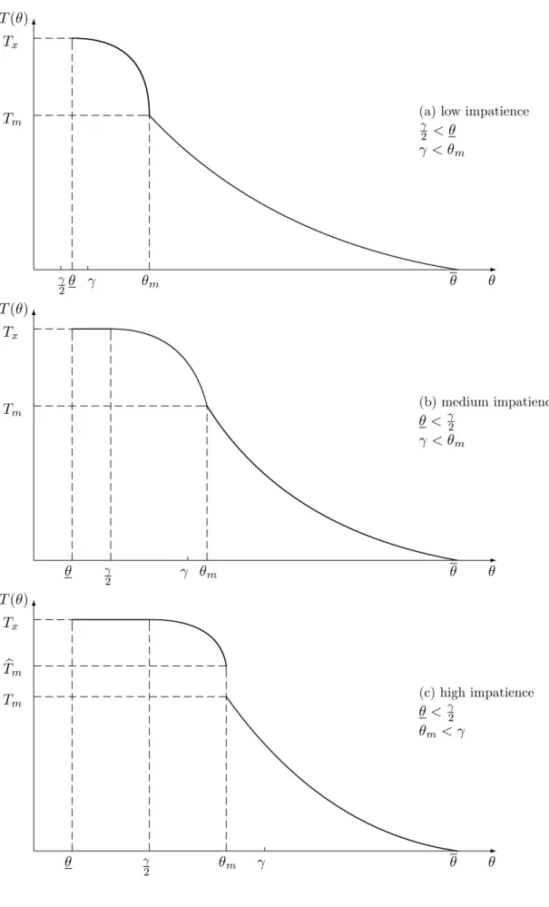
3.4 Summary of the results
Our results are summed up in Figure 1, which shows the concession function on the whole range ; ; and therefore the solution of the stabilization game.
For 2 m; , the optimal stabilization date is the interior solution of the …rst game, in
which the greenest country stabilizes alone; it is a decreasing function of , from Tm to 0; and
it is convex (Proposition 1).
So stabilization by a single country, the greenest, occurs only if this country is green enough, which means that it has a parameter of preference for the environment greater than m: The
value of m itself depends on the BAU emissions of pollution, the initial environmental quality
and the impatience of the countries. The worst the initial conditions and the more impatient the countries, the greener the greenest country has to be. The higher ; the faster the stabilization of environmental quality.
For 2 [ ; m[, the optimal stabilization date is the solution of the second game, in which
both countries reduce their pollution (Proposition 3). Three cases can then occur (Proposition 2). They are depicted in Figure 1, where they are obtained by making the discount rate vary, other things being equal.
In case (a), impatience is low ( < m and =2 < ), and the con…guration of parameters
such that in the second game the interior solution prevails. The optimal stabilization is a decreasing function of ; from Tx to Tm. We could not obtain a formal result for the concavity
of this function, but numerical simulations show us that it is concave most of the time.
In case (b), impatience is medium ( < mbut =2 > ), and the con…guration of parameters
such that there exists an accumulation of concessions at Tx: If the greenest country has a
parameter of preference for the environment between and 2; both will rationally let the natural capital reach its minimum level.
Finally, in case (c), impatience is high ( > m and =2 > ), and the con…guration of
parameters such that there exists an accumulation of concessions at Tx but also a jump in the
whatever its parameter of preference for the environment.
So if the greenest country is not green enough, both countries wait until it is impossible for one of them to stabilize alone. Then the occurence of the stabilization depends on the comparison of the smallest preference for the environment and the half of the discount rate. If impatience is so low that 2 , the greenest country reduces its pollution to zero and the other one does the rest of the job of stabilization. When impatience is high (2 > ), the same thing occurs if the greenest country is green enough ( > 2), but a complete depletion of environmental quality is optimal if it is not the case.
4
Conclusion
Due to the absence of a supra-national authority able to monitor the emergence and implemen-tation of a coordinated pollution abatement program, the world is likely to be trapped in lasting excessive pollution, due to non-cooperative national policies. We have shown, in the war of at-trition framework, that the excess of pollution will be all the more persistent since the greenest of the two countries is less green, the initial conditions are adverse (high business-as-usual pollu-tion and low initial environmental quality), the countries are optimistic concerning the possible range of the preference parameters, and impatience corrected for natural regeneration is high. We have also shown that it can be rational for the greenest country to wait so long that it cannot stabilize alone. Furthermore, it is also possible that stabilization never occurs.
Natural possible extensions are the following. First, the representation of the economy, the environment, and their interactions could be less oversimpli…ed. For instance, empirical studies show that the regeneration rate is not a constant but depends on the level of environmen-tal quality itself. If natural regeneration slows down as environmenenvironmen-tal quality diminishes, the threshold constituted by impatience corrected for natural regeneration increases, making stabi-lization more likely. Secondly, we could introduce more asymmetry between the players, which are here identical except for their preference for the environment. For instance, they could have di¤erent social discount rates (one country could be more impatient than the other), or di¤erent
business-as-usual levels of polluting activities. Thirdly, it would obviously be very interesting to extend this framework to the case of more than two countries, in the spirit of generalized war of attrition models (cf. Bulow and Klemperer, 1999). The global warming problem for example could be better studied in a framework considering three di¤erent groups of countries, the United States, the signatories of the Kyoto Protocol, and the developing countries.
References
Alesina, A. and A. Drazen, 1991, Why are stabilizations delayed?, American Economic Review 81(5), 1170–1188.
Bac, M., 1996, Incomplete information and incentives to free ride on international environmental resources, Journal of Environmental Economics and Management 30, 301–315.
Barrett, S., 1994, Self-enforcing international environmental agreements, Oxford Economic Pa-pers 46, 878–894.
Barrett, S., 1998, Political economy of the Kyoto Protocol, Oxford Review of Economic Policy 14(4), 20–39.
Bliss, C. and B. Nalebu¤, 1984, Dragon-slaying and ballroom dancing: the private supply of a public good, Journal of Public Economics 25(1–2), 1–12.
Bulow, J. and P. Klemperer, 1999, The generalized war of attrition, American Economic Review 89(1), 175–189.
Carraro, C. and D. Siniscalco, 1993, Strategies for the international protection of environment, Journal of Public Economics 52(3), 309–328.
Carré, M., 2000, Debt stabilization with a deadline, European Economic Review 44, 71–90. Casella, A. and Eichengreen, 1996, Can foreign aid accelerate stabilization?, The Economic Journal 106, 605–619.
Chander, P. and H. Tulkens, 1992, Theoretical foundations of cost sharing in transfrontier pollution problems, European Economic Review 36, 388–399.
Chander, P. and H. Tulkens, 1995, A core-theoretic solution for the design of cooperative agree-ments on transfrontier pollution, International Tax and Public Finance 2, 273–294.
Dockner, E.J. and N. van Long, 1993, International pollution control, cooperative versus non-cooperative strategies, Journal of Environmental Economics and Management 25, 13–29. Hoël, M., 1992, International environmental conventions: the case of uniform reductions of emissions, Environmental and Resource Economics 2, 141–159.
-6 m 2 T ( ) Tx
Tm (a) low impatience
2 < < m -6 m 2 T ( ) Tx Tm (b) medium impatience < 2 < m -6 m 2 T ( ) Tx Tm b Tm (c) high impatience < 2 m <