A microfluidic device for digital manipulation of gaseous samples

HAL Id: hal-03064972

https://hal.archives-ouvertes.fr/hal-03064972

Submitted on 14 Dec 2020

HAL is a multi-disciplinary open access archive for the deposit and dissemination of sci-entific research documents, whether they are pub-lished or not. The documents may come from teaching and research institutions in France or abroad, or from public or private research centers.

L’archive ouverte pluridisciplinaire HAL, est destinée au dépôt et à la diffusion de documents scientifiques de niveau recherche, publiés ou non, émanant des établissements d’enseignement et de recherche français ou étrangers, des laboratoires publics ou privés.

A microfluidic device for digital manipulation of gaseous

samples

A. Enel, A. Bourrelier, J. Vial, Didier Thiebaut, B. Bourlon

To cite this version:

A. Enel, A. Bourrelier, J. Vial, Didier Thiebaut, B. Bourlon. A microfluidic device for digital manip-ulation of gaseous samples. Lab on a Chip, Royal Society of Chemistry, 2020, 20 (7), pp.1290-1297. �10.1039/C9LC01163C�. �hal-03064972�

A microfluidic device for digital manipulation of gaseous samples

1 2

A. Enel1_{, A. Bourrelier}1_{, J. Vial}2_{, D. Thiébaut}2_{, and B. Bourlon}1

3

1 _{Univ. Grenoble Alpes, CEA, LETI, MINATEC Campus, F-38000 Grenoble, France}

4

2 _{UMR8231 CBI, LSABM, ESPCI Paris–CNRS, PSL Institute, Paris, France}

5 E-mail: [email protected] 6 7

Abstract

Digital microfluidics is known for fine manipulation of sub-millimeter samples, with applications from 9

biological sample preparation to diagnostic testing. Unfortunately, until now, it is only limited to liquid 10

phases. In this paper, we present a new system based on a digital microfluidic platform (DMFP), which 11

is able to digitally manipulate gaseous samples, such as alkanes from n-hexane to n-nonane. The DMFP 12

relies mostly on interconnected micropreconcentrators (µPC) to trap and release the samples 13

depending on their controlled temperature. We show that the DMFP is capable to perform all basic 14

operations of digital microfluidics: trapping/releasing and moving samples, adding samples and 15

separating samples, i.e. making a substraction. As a first example of more complex programmable use 16

of our DMFP, we measured the breakthrough volume of alkanes on Tenax TA adsorbent. The results 17

were consistent with tabulated values obtained with standard laboratory instruments. Such DMFP 18

promises great possibilities for more complex programmable gas microfluidics digital devices and the 19

development of new digital gas sample preparation and analysis methods. 20

21

Keywords

22

Digital microfluidics; gas samples preparation and analysis; silicon microfabrication; miniaturization; 23 preconcentrator 24 25

Introduction

Over the past decade, microfluidics, defined as the manipulation of fluids at small scale, mainly sub-27

millimeter scale, have steadfastly progressed 1–12_{. It is also compounded by the understanding of the}

28

fluid mechanics at this scale, the chemical interactions and the microfabrication techniques mandatory 29

to craft these devices. The development of microfluidics has yielded several techniques of small-scale 30

fluid control, for example efficient and reproducible droplet generation by making two immiscible 31

liquids flow through specific shapes. This technique is very useful: droplets are almost a closed 32

medium, as diffusion to the surrounding fluid is very low, and allows for encapsulation of useful 33

substances, such as enzymes for enzymatic assays13_{. Another technique emerged, among lots of}

34

others: electrowetting, more specifically electrowetting on a dielectric (EWOD). In this mode, two 35

electrodes are used to create an electric field on a dielectric, which changes the wettability of the 36

dielectric and so the contact angle of the droplet. This change allows for movement or immobilization 37

of the droplet. It is then possible to make a grid with these electrodes, and move droplets at will on 38

this grid. These two techniques paved the way for digital microfluidics: microfluidics programmable by 39

analogy to a digital computer. This means that the droplets are commanded by a set of simple 40

instructions, from known state to known state while a clock is used to synchronize the system. This 41

leads to several operations such as moving, trapping, mixing or merging, storing, and extraction of 42

surrounding fluid. Several devices also use bubbles surrounded by liquid14,15_{. To our knowledge, no}

44

digital microfluidic device has been made to manipulate gas samples within a carrier gas. 45

In the meantime, developments in miniaturization of air analysis devices have yielded 46

micropreconcentrators16–18 _{(µPC). These devices consist of a chamber containing an adsorbent, a}

47

heating element and a temperature probe. It is then possible to trap a gas on the adsorbent, or release 48

it at will by changing the µPC temperature. When the compound of interest is trapped on the µPC, it 49

does not diffuse within the surrounding gas. These characteristics make µPC a suitable building block 50

for digital microfluidics. Digital microfluidics for gases could help to design programmable, automatic 51

and versatile gas sample preparation and analysis systems. These systems could be free from diffusion 52

related issues that are met in conventional instruments19_{. They could also allow sample manipulation}

53

without losses. As applications, such devices could be combined with conventional analytical 54

techniques or open new approaches for portable miniaturized instruments. 55

In this work, a digital microfluidic platform (DMFP) using pumps, µPC and a detector was assembled. 56

We showed that the digital manipulation of gas samples was possible with the DMFP, and 57

demonstrated all elementary operations: trapping/releasing and moving a compound, merging two 58

compounds and separating two compounds. Several alkanes, ranging from n-hexane (C6) to n-nonane 59

(C9) were used to demonstrate these operations. These elementary operations were carried-out by 60

controlling precisely, step by step, the state of the pumps and the temperature of the µPCs. These 61

elementary operations were also the first step towards a more complex device, which could be used 62

to perform high-level functions, such as separation of mixed samples. 63

As a first proof of concept of a more complex programmable application, the DMFP was used to 64

measure the breakthrough volume of these alkanes on a classical adsorbent (Tenax TA). Breakthrough 65

volume measurements with standard laboratory instruments, such as a gas chromatograph, are labor 66

intensive, as they need several injections, one for each temperature studied. As an illustration of 67

potential applications, it was possible to measure automatically with the DMFP the breakthrough 68

volume on a wide range of temperatures using only one injection, by manipulating without loss the 69

same initial gas sample. 70

Experimental

Components fabrication

The micropreconcentrator chip fabrication has been already described elsewhere 20,21_{. The size of the}

74

µPC chip was 21 mm x 7.6mm. On the front side of the silicon chip, 400 μm deep inlet/outlet and a 75

central cavity were etched in silicon, and sealed with a Pyrex glass. The 6.6 µL cavity was filled with 76

Tenax-TA adsorbent powder, a polymer of 2,6-diphenylphenol. Tenax TA is widely used for trapping 77

volatile organic compounds from air samples. Inlet/outlet of the chip were glued to nickel capillaries. 78

On the back side of the chip Ti/Pt thin film heaters and thermoresistive probes were deposited. Several 79

other similar designs have been reported in the literature 22–24_.

80

The micro thermal conductivity detectors (µTCD) were also batch processed on 200 mm silicon wafers. 81

The size of the µTCD chip was 9.6 mm x 5.4 mm. Two 100μm deep 200µm wide microchannels were 82

etched in the silicon chip by anisotropic deep reactive ion etching (DRIE) following by isotropic plasma 83

etching. Each channel contained two suspended membranes. Each membrane was made of 200 nm 84

thin silicon nitride membrane on which a platinum thermoresistive conductor had been deposited by 85

sputtering. The other half of microchannels was etched by wet etching on a Pyrex glass that was finally 86

sealed on top of the silicon wafer. The µTCD was then glued and wire-bonded to a printed circuit board 87

holder. 80 µm inner diameter and 150 µm outer diameter fused silica capillaries were then glued in 88

the inlets/outlets of the silicon chip microchannels. The membranes were then connected electrically 89

in a Wheatstone bridge structure. Several similar other designs have been reported in the 90

literature25,26_.

91

When the µTCD is functioning, the membranes are heated and thermal exchanges with the 92

surrounding gas reach a stationary state. If the surrounding gas changes its thermal conductivity, for 93

example by changing its chemical composition, the thermal exchanges are disrupted. This causes the 94

membranes to change their temperatures, and their resistance. This changes the output of the 95

Wheatstone bridge, which is monitored. The µTCD output is then related to the concentration of the 96

sample inside the carrier gas. When samples go through the µTCD, the resulting signal has the shape 97

of a peak. The peak’s height is related to the concentration of the sample, and its area to the amount 98

of sample. 99

The µTCD was checked for linearity: as expected, the area of the peaks scaled linearly with the amount 100

of sample within the studied range. The results are available in the supplementary data. 101

102

Experimental setup

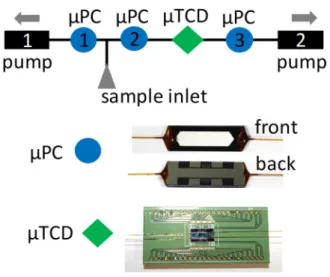
103

The schematics of the DMFP are presented in Figure 1. 104

105

106 107

As shown on Figure 1, the DMFP contained three µPC and one µTCD, with two pumps linked to them. 108

The pumps were not miniaturized, but the main building bricks of the system were. The pumps may 109

be miniaturized in the future, as such pumps have already been reported27_{. No valves were used here,}

110

however miniaturized valves have been reported28_{. Pumps were Xavitech models (V200-O2C12V) and}

111

connected to the DMFP with Tygon® tubes (1/6’’ outer diameter, 1/10’’ inner diameter). The carrier 112

gas used to move samples inside the DMFP was ambient air. 1/16’’ unions were used to connect the 113

components together, with 1/16’’ ferrules and nuts. The µTCD was connected between the µPC2 and 114

µPC3 using one of its two gas channels (as analytical channel); the second µTCD gas channel was 115

connected between µPC3 and pump 2 (as reference channel) to lower the baseline drift. The second 116

reference connection is not shown in the Figure 1 for simplification. A fused silica capillary, 1.50m x 117

250µm inner diameter, was used to connect the µPC2 to the µTCD. This capillary was found to reduce 118

artefacts on the µTCD signal. The artefacts were caused by transitory states during the heating of a 119

µPC or the pumps starting. They appeared close to the sample peak, disturbing the baseline. The 120

pumps and µPC were powered by a 12 V supply device, and the µTCD by a 9 V battery. An electronic 121

setup connected to a computer through USB allowed to control the pumps, the µPC heaters as well as 122

to acquire signal from the µTCD and the µPC temperature probes. Labview 2012 was used to program 123

and control the sequence of states of the DMFP, as well as acquire and register the data. 124

Samples could be injected on either µPC1 or µPC2 by pumping with pump 1 or pump 2 respectively. 125

Samples were prepared by injecting a few microliters of liquid sample inside a Tedlar® bag of 1 L 126

(Supelco, 24633) filled with 5.0 nitrogen (Air Liquide). The samples used were n-hexane (C6) (Carlo 127

Erba, 99% HPLC grade), n-heptane (C7) (99 % anhydrous, Sigma Aldrich), n-octane (C8) (≥99% 128

anhydrous, Sigma Aldrich) and n-nonane (C9) (≥ 99 % anhydrous, Sigma Aldrich). Prior to injection, the 129

bag was cleaned by filling it 3 times with 5.0 nitrogen and emptying with a vacuum pump. After 130

injection of the sample in the bag, the bag was let at room temperature for 15 minutes to equilibrate. 131

For the injection of samples, the Tedlar® bag was connected to the inlet of the T-junction. The 132

connection was made with a 1/16’’ stainless steel capillary. Several samples were prepared: C6 5 ppm, 133

C7 10 ppm, C7 5 ppm, C9 5 ppm, C7-C9 5 ppm, C6 1 ppm, C7 1 ppm, C8 1 ppm, C9 1 ppm. Mass flow 134

rates inside the DMFP were around 0.30 mL/min. 135

136

Results and discussion

137 138

The manipulation of gaseous samples relies mostly on the adsorption/desorption of compounds using 139

adsorbent packed in the µPCs. The compounds are trapped on the adsorbent and released when the 140

µPC is heated. Using pumps, it is possible to control the gas flow and thus the samples displacement. 141

Trapping and preconcentration

142

The ability of our µPC to trap compounds was checked using n-hexane (5 ppm). C6 was first loaded on 143

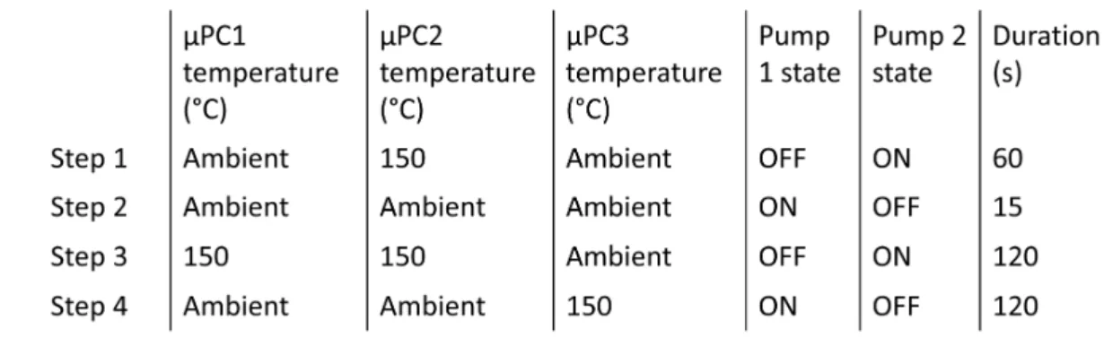
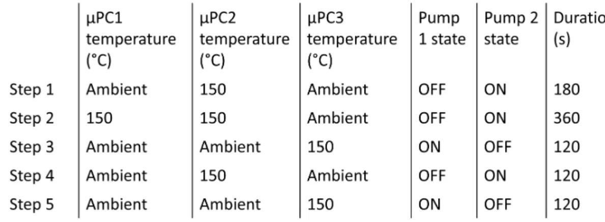
µPC2 before starting the experiment. Table 1 presents the DMFP program used for this experiment. 144

145

Table 1 : Program of the DMFP used for the preconcentration experiment. On every step 2 a Tedlar bag containing C6 in

146

nitrogen was connected to the injector to load C6 on µPC1.

147

On step 1, the sample moved from µPC2 to µPC3. On step 2, the Tedlar bag containing C6 5 ppm was 148

plugged to the injector: supplementary C6 was loaded on µPC1. The bag was then plugged out and the 149

injector closed. On step 3, the supplementary C6 moved from µPC1 to µPC3. On step 4, the sample 150

moved to µPC2. 151

Results are shown on Figure 2. 152

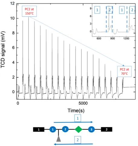
153

Figure 2 : Concentration of 5 ppm n-hexane in nitrogen on µPC2.The 4 steps are indicated by the numbers on the figure: Step

154

1 was the movement of the sample from µPC2 to µPC3. Step 2 was the loading of the sample on µPC1. Step 3 was the

155

movement of the sample from µPC1 to µPC3. Step 4 was the movement of the sample from µPC3 to µPC2. Step 1,2,3,4 were

156

repeated 4 times in total. Each time the compound went through the µTCD a signal (peak) is produced. The height of the C6

157

peak increased on every cycle, meaning C6 was effectively being concentrated.

158

As shown in Figure 2, µPCs are very effective at concentrating compounds, trapping them and releasing 159

them on demand. During each step 3, the height and area of the C6 peak was the same, indicating the 160

amount of C6 loaded during step 2 was constant. During each step 1 and step 4, the height and area 161

of the n-hexane peak rose, meaning the amount of C6 trapped on µPC3 was increasing. This is 162

consistent with the fact that C6 was trapped on the µPC3 and could be released on demand, and that 163

more C6 was added to the DMFP at each step 2. 164

165

Controlled movements of samples

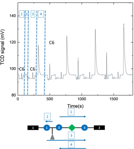
166

The sample, C7 (10 ppm), was loaded on µPC2, and then moved back and forth 20 times between µPC2 167

and µPC3. Table 2 shows the DMFP program used for this experiment. It consisted of two steps: step 168

1 consisted in heating µPC2 with pump 2 on: the sample was carried to µPC3. Step 2 consisted in 169

heating µPC3 with pump 1 on: the sample was carried to µPC2. 170

171

Table 2 : Program of the DMFP used for the controlled movements experiment.

172

Figure 3 shows the TCD signal collected during a sequence of 20 movements of the sample. 173

174

Figure 3 : Controlled movement of n-heptane 10 ppm between µPC2 and µPC3. Two steps were done: on step 1, µPC2 was

175

heated to 150°C for 30 s and n-heptane went to µPC3. µPC2 cooled down for 40 s. On step 2, µPC3 was heated to 150°C and

176

n-heptane went to µPC2. µPC3 cooled down for 40s. See the inset for a more detailed view of the steps. Steps 1 and 2 were

177

then repeated 20 times. A signal peak was observed every time n-heptane went through the µTCD.

178

Figure 3 shows that the sample could be moved 20 times without significant losses over time due to 179

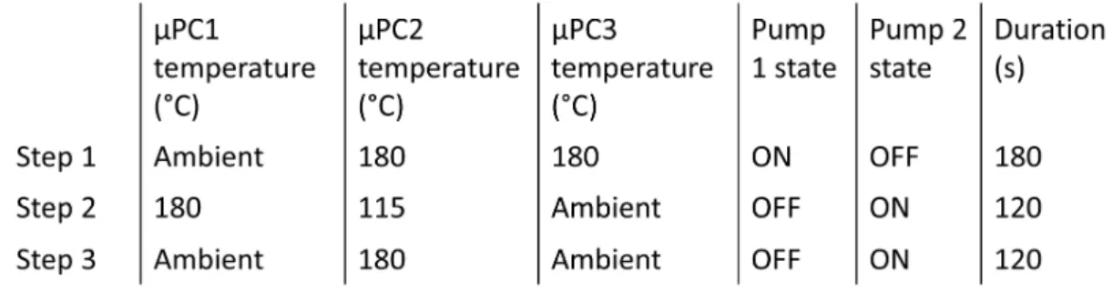
diffusion, or non-efficient trapping. Indeed, the peaks obtained during the 20 steps 1 looked similar, 180

with an area distribution of 4583 ± 683 mV*s. The peaks obtained during the 20 steps 2 also looked 181

similar: their area distribution was 7063 ± 1226 mV*s. This means the µPC was effective at trapping 182

compounds, and managed to release them efficiently when heated. However, one can notice a slight 183

variation in the height of the peaks obtained during step 1 and the height of the peaks obtained during 184

step 2 was observed, certified by a statistical test. This variation could be attributed to the fused silica 185

capillary between PC2 and the µTCD: its volume was 75 µL, compared to the 1.5 µL capillary volume 186

between PC3 and the µTCD. The sample diffused more when traveling through the 75 µL, causing a 187

decrease in local concentration and thus a decrease in the µTCD peak signal. The amplitude of this 188

variation was low and did not hinder the conclusions. This could be investigated and solved in a future 189

setup if needed. 190

Mixing two different compounds

191

It was also possible to use this device to mix two compounds. To demonstrate this, µPC1 and µPC2 192

were loaded with C9 (5 ppm) with C7 (5 ppm), respectively. The compounds were added on µPC3 and 193

then moved back and forth between µPC2 and µPC3. The Table 3 shows the DMFP program used for 194

this experiment. 195

196

Table 3 : Program used for the C7-C9 addition experiment.

197

The results are shown on Figure 4. 198

Figure 4 : Addition of n-heptane 5 ppm with n-nonane 5 ppm. The peaks are labelled on the figure. Each time a compound

200

went through the µTCD a signal peak was observed. The peaks observed at 600 s, 800 s and 900 s were a combination of the

201

peaks observed at 80 s (C7), and the peak observed at 480 s (C9). To move compounds, the µPCs were heated to 150°C.

202

Figure 4 shows that the two compounds, C7 and C9, produced, visually, different peaks when they 203

went through the µTCD. C7 went through the µTCD on step 1; C9 went through on step 2. On step 3 204

both of them were added on µPC3, the resulting peak being the sum of the two individual peaks. This 205

meant that the addition was successful, and the two compounds could move together during steps 4 206

and 5: they did not separate on their own. 207

208

Separating different compounds

209

Using the DMFP it was also possible to separate two different compounds. To show this, C7-C9 5 ppm 210

was loaded on µPC1, and then moved on µPC3 during a preliminary step, which is not shown. 211

A three-step procedure was then performed: on step 1, µPC2 and µPC3 were heated to 180°C: the 212

sample moved from µPC3 to µPC1. On step 2, µPC2 was set to 115°C and the mix C7-C9 moved from 213

µPC1 to µPC3. As the mix went through µPC2, the separation was performed: 115°C was hot enough 214

for C7 to move through, but too cold for C9, which was not volatile enough to be displaced. C9 was 215

trapped on µPC2. On step 3, µPC2 was then heated to 180°C to release C9. The DMFP program used 216

for this experiment is shown in Table 4. 217

218

Table 4 : DMFP program used for the C7-C9 separation experiment.

219 220

The results are shown on Figure 5. 221

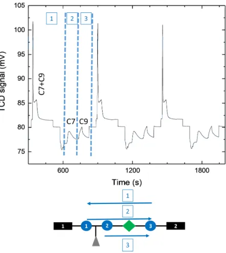
222

Figure 5 : Separation of C7 and C9. C7 and C9 were first loaded on µPC1. A preliminary step was done to move the sample

223

from µPC1 to µPC3. This step is not shown. Three steps were done: on step 1, the C7-C9 mix was pumped to µPC1, µPC2 and

224

µPC3 were heated to 180°C. On step 2, µPC2 was set to 115°C and the mix went to µPC2. 115°C was hot enough for C7 to go

225

through µPC2 and not be trapped: it went through the µTCD to µPC3. C9 is not volatile enough and was trapped on µPC2. On

226

step 3, µPC2 was heated to 180°C: C9 was released and went to µPC3 through the µTCD. Steps 1, 2 and 3 were then repeated

227

twice.

228

Figure 5 shows that the separation was effective: by keeping µPC2 at 115°C C7 was able to go through 229

but C9 was trapped. C9 was only released by heating µPC2 at 180°C. Three successive successful 230

separations showed the process was repeatable. As co-elutions between C7 and C9 might be possible, 231

control experiments were done by analysing C7 5 ppm and C9 5 ppm with the same program shown in 232

Table 4. Results are shown on Figure 6. 233

234

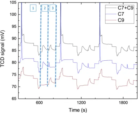
Figure 6: Separation of C7 5 ppm and C9 5 ppm. The program is the same as shown on Table 4. For the black trace, both C7 5

235

ppm and C9 5 ppm were loaded on µPC1. For the blue trace, only C7 5 ppm was loaded. For the red trace, only C9 5 ppm was

236

loaded.

237

Figure 6 shows that the separation was quite effective, as C9 was totally trapped on µPC2 during step 238

2. However, the separation was not complete: a small amount of C7 went through the µTCD during 239

step 3, meaning it was trapped on µPC2 during step 2. By measuring the peak area, around 11% of the 240

total C7 amount was trapped on µPC2 during step 2 and 89% of the amount went through. The DMFP 241

could not perform a perfect single-step separation, but it is still capable of separating different 242

compounds, which is one of the basics operations of digital microfluidics. The performances could be 243

enhanced by repeating the separation step. 244

Measuring breakthrough volumes

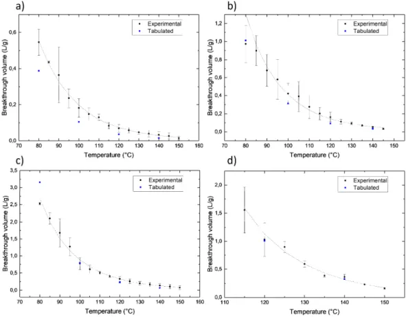
245

The DMFP was used to measure breakthrough volumes (BV) on alkanes ranging from hexane to n-246

nonane (C9). With standard laboratory instruments, BV studies requires multiple samplings, injections 247

and analyses, as the sample is lost after each analysis. The DMFP used the same sample that was 248

digitally manipulated to gather in about 10 minutes the data needed for one BV measurement at a 249

specific temperature. As the BV was assessed automatically for one compound with the DMFP on a 250

wide range of temperatures in one experiment, the experiment duration was about 3 hours. The BV is 251

the volume of carrier gas needed to elute 50% of the analyte through the adsorbent, at a specific 252

temperature. It is expressed in liters/ grams of adsorbent. The BV is an intrinsic value, which can be 253

tabulated. It characterizes the strength of the interaction between one compound and one adsorbent. 254

At constant flow rate of carrier gas, the BV only changes with temperature for a couple 255

analyte/adsorbent: as temperature increases, the BV decreases due to the adsorption equilibrium 256

shifting towards the desorption of the analyte. The BV tables are useful to assess which adsorbent to 257

use for a specific target, and the range of temperatures in which the target is trapped or released. 258

During these experiments, the sample was loaded on µPC1. The experiments then consisted in two 259

steps: at step 1, µPC1 was heated to 150°C and µPC2 to a selected temperature, ranging from 150°C 260

to 70°C. Pump 2 was switched on for 300 s. At step 2, µPC3 and µPC2 were heated to 150°C. Pump 1 261

was switched on for 60 s. Every time step 1 was repeated, µPC2 temperature was lowered by 5°C. 262

Table 5 shows the DMFP program used for this experiment. 263

264

Table 5 : DMFP program used for the C6 breakthrough experiment.

265 266

Figure 7 shows a typical breakthrough experiment. 267

268

Figure 7: Breakthrough curve of 1 ppm n-hexane in nitrogen. The baseline drift and its offset were corrected. Every intense

269

peak observed at step 2 showed the movement of C6 to µPC1 from µPC3, meaning breakthrough occurred. See the inset: the

270

peak observed at 545 s was the breakthrough of C6 through µPC2 at 150°C during step 1. The peak observed at 817 s was the

271

return of C6 from µPC3 to µPC1 during step 2. Every time step 1 was repeated, µPC2 temperature was lowered by 5°C.

272

Figure 7 shows that breakthrough happened over a wide range of temperatures, as evidenced by a 273

peak observed during step 1. The peak observed during step 2 was a second proof of a breakthrough: 274

if it appeared, it meant C6 came back to µPC1 from µPC3. It was only possible if C6 managed to reach 275

µPC3 during step 1 and went through µPC2. 276

As temperature of µPC2 was decreased during the experiment, breakthrough became less 277

pronounced. This breakthrough efficiency loss is shown in step 2: the peak observed during step 2 278

became less and less intense. For low temperatures, breakthrough did not occur and there was no 279

peak observed during step 2, such as, in the C6 case shown on Figure 7, the steps done below 75°C. 280

During this experiment, the setup was not opened, meaning only a single sample was loaded and then 281

travelled during the duration of the whole experiment. 282

For several alkanes the experiment did not yield values for every temperature in the range, as the BV 283

was too high compared to the volume pumped through the µPC. BV values were normalized by 284

subtracting the dead volume, measured at the start of every experiment by doing a breakthrough at 285

180°C with the sample. At this temperature, analytes were not retained on the adsorbent. Data were 286

then fitted according to Kroupa et al. 29_{. They proposed a two or three parameters model for the}

287

dependence of the BV with the temperature. One of the parameters is directly related to the 288

adsorption enthalpy of the compound on the adsorbent, which is an intrinsic characteristic of the 289

compound/adsorbent interaction. 290

Figure 8 shows the measured breakthrough volume for C6, C7, C8 and C9. 291

292

Figure 8: Breakthrough volume measured for a) C6, b) C7, c) C8 and d) C9. Experiments were made in duplicate.

293

Figure 8 shows that the fit, according to the model proposed by Kroupa et al.29 _{, of the BV as a function}

294

of the temperature was in good agreement with the measured data for all of the analysed samples. It 295

was also possible to measure the adsorption enthalpy of C6 on Tenax at 25°C : the measured value of 296

-46.8 ± 15.0 kJ/mol was in the same order of magnitude as the value of -23.8 kJ/mol obtained by 297

Kroupa et al29_.

298

Data were also compared with tabulated values found on SIS website30 _{: a slight deviation was}

299

observed from tabulated values. This deviation was consistent with Kroupa et al. findings29 _{: they}

300

attributed the deviation to a fitting error in SIS interpolations. 301

Conclusion

302

The digital microfluidic platform presented in this study allows step by step programmable digital 303

manipulations of gas samples without losses. All elementary operations (trapping/releasing, moving, 304

mixing, and separating samples) have been demonstrated using n-hexane to n-nonane alkanes. 305

Moreover, by programming a succession of elementary operations, it is possible to perform more 306

complex operations and applications. This could be a first step towards digital chromatography, since 307

the elementary operations performed by the DMFP presented here can be related to a single 308

theoretical plate as in Martin and Synge theory31_{. As a first illustration, the measurements of}

309

breakthrough volumes of gases have been performed. The results were in agreement with the 310

tabulated values obtained with standard laboratory instruments, and showed good agreement with 311

fundamental values, such as the adsorption enthalpy of the gases on the adsorbent. 312

Beyond this first DMFP made of three µPC, other DMFP with more complex network of µPC could be 313

developed in the future. With the development of a more complex DMFP and gas manipulation 314

algorithm, this work could lead to new miniaturized digital systems and methods for gas sample 315

preparation and analysis. These new methods of sample handling would be suitable for portable gas 316

analysis systems, but also conventional gas analysis systems. For example, a digital sample handler 317

could be used to extract compounds within a certain volatility range from a gas sample prior to 318

injection in a conventional gas chromatograph. As another example, a system similar to the DMFP 319

presented here could be used as an online miniaturized trap for chromatographic applications in a 320

similar fashion to thermal modulators for comprehensive bi-dimensional gas chromatography. 321

322

Bibliography

323

1 M. G. Pollack, V. K. Pamula, V. Srinivasan and A. E. Eckhardt, Expert Rev. Mol. Diagn., 2011, 11, 324

393–407. 325

2 M. Ibrahim and K. Chakrabarty, Proc. IEEE, 2018, 106, 1717–1743. 326

3 Y. Fouillet, D. Jary, C. Chabrol, P. Claustre and C. Peponnet, Microfluid. Nanofluidics, 2008, 4, 159– 327

165. 328

4 R. B. Fair, Microfluid. Nanofluidics, 2007, 3, 245–281. 329

5 S.-Y. Teh, R. Lin, L.-H. Hung and A. P. Lee, Lab. Chip, 2008, 8, 198. 330

6 F. Mugele and J.-C. Baret, J. Phys. Condens. Matter, 2005, 17, R705–R774. 331

7 A. Wego, S. Richter and L. Pagel, J. Micromechanics Microengineering, 2001, 11, 528. 332

8 C. D. Chin, V. Linder and S. K. Sia, Lab Chip, 2007, 7, 41–57. 333

9 P. Yager, T. Edwards, E. Fu, K. Helton, K. Nelson, M. R. Tam and B. H. Weigl, Nature, 2006, 442, 334

412–418. 335

10 A. Manz, N. Graber and H. M. Widmer, Sens. Actuators B Chem., 1990, 1, 244–248. 336

11 R. Malk, Y. Fouillet and L. Davoust, Sens. Actuators B Chem., 2011, 154, 191–198. 337

12 M. G. Pollack, A. D. Shenderov and R. B. Fair, Lab. Chip, 2002, 2, 96–101. 338

13 V. Srinivasan, V. K. Pamula and R. B. Fair, Anal. Chim. Acta, 2004, 507, 145–150. 339

14 Y. Zhao and S. K. Cho, Lab Chip, 2007, 7, 273–280. 340

15 P. Garstecki, I. Gitlin, W. DiLuzio, G. M. Whitesides, E. Kumacheva and H. A. Stone, Appl. Phys. 341

Lett., 2004, 85, 2649–2651.

16 M. Li, S. Biswas, M. H. Nantz, R. M. Higashi and X.-A. Fu, Sens. Actuators B Chem., 2013, 180, 130– 343

136. 344

17 M.-S. Chae, J. Kim, Y. Yoo, J. Kang, J. Lee and K. Hwang, Sensors, 2015, 15, 18167–18177. 345

18 B. Alfeeli and M. Agah, IEEE Sens. J., 2009, 9, 1068–1075. 346

19 J. J. Van Deemter, F. J. Zuiderweg and A. van Klinkenberg, Chem. Eng. Sci., 1956, 5, 271–289. 347

20 T. H. Chappuis, B. A. Pham Ho, M. Ceillier, F. Ricoul, M. Alessio, J.-F. Beche, C. Corne, G. Besson, J. 348

Vial, D. Thiébaut and B. Bourlon, J. Breath Res., 2018, 12, 046011. 349

21 B. Bourlon, B.-A. P. Ho, F. Ricoul, T. Chappuis, A. B. Comte, O. Constantin and B. Icard, in SENSORS, 350

2016 IEEE, IEEE, 2016, pp. 1–3.

351

22 M. Akbar and M. Agah, J. Microelectromechanical Syst., 2013, 22, 443–451. 352

23 B. Alfeeli, V. Jain, R. K. Johnson, F. L. Beyer, J. R. Heflin and M. Agah, Microchem. J., 2011, 98, 240– 353

245. 354

24 B. Alfeeli, L. T. Taylor and M. Agah, Microchem. J., 2010, 95, 259–267. 355

25 F. Feng, B. Tian, L. Hou, Z. Yu, H. Zhou, X. Ge and X. Li, in 2017 19th International Conference on 356

Solid-State Sensors, Actuators and Microsystems (TRANSDUCERS), 2017, pp. 1433–1436.

357

26 S. Narayanan and M. Agah, J. Microelectromechanical Syst., 2013, 22, 1166–1173. 358

27 C. G. J. Schabmueller, M. Koch, M. E. Mokhtari, A. G. R. Evans, A. Brunnschweiler and H. Sehr, J. 359

Micromechanics Microengineering, 2002, 12, 420.

360

28 K. Nachef, F. Marty, E. Donzier, B. Bourlon, K. Danaie and T. Bourouina, J. Microelectromechanical 361

Syst., 2012, 21, 730–738.

362

29 A. Kroupa, J. Dewulf, H. Van Langenhove and I. Vı ́den, J. Chromatogr. A, 2004, 1038, 215–223. 363

30 Hydrocarbon Breakthrough Volumes for Adsorbent Resins, 364

https://www.sisweb.com/index/referenc/bv-hyd.htm. 365

31 A. J. Martin and R. L. Synge, Biochem. J., 1941, 35, 1358. 366

367 368