Dealing with missing data in family-based association studies: a multiple imputation approach

HAL Id: inserm-00143682

https://www.hal.inserm.fr/inserm-00143682

Submitted on 4 Sep 2009

HAL is a multi-disciplinary open access

archive for the deposit and dissemination of sci-entific research documents, whether they are pub-lished or not. The documents may come from teaching and research institutions in France or abroad, or from public or private research centers.

L’archive ouverte pluridisciplinaire HAL, est destinée au dépôt et à la diffusion de documents scientifiques de niveau recherche, publiés ou non, émanant des établissements d’enseignement et de recherche français ou étrangers, des laboratoires publics ou privés.

Dealing with missing data in family-based association

studies: a multiple imputation approach

Emmanuelle Génin, Pascal Croiseau, Heather Cordell

To cite this version:

Emmanuelle Génin, Pascal Croiseau, Heather Cordell. Dealing with missing data in family-based association studies: a multiple imputation approach. Human Heredity, Karger, 2007, 63 (3-4), pp.229. �inserm-00143682�

Dealing with missing data in family-based association studies:

a multiple imputation approach

Pascal Croiseau (1), Emmanuelle Génin (1), Heather J. Cordell (2) (1) INSERM U535, FRANCE

(2) Institute of Human Genetics, Newcastle University, UNITED KINGDOM

Corresponding author: Pascal Croiseau

Genetic Epidemiology and Structure of Human Populations INSERM U535, BP10000

94817 VILLEJUIF cedex

tel. +33 1 45 59 52 40, E-Mail croiseau@vjf.inserm.fr

Key words : case-parent trio, missing data, multiple imputation, conditional logistic regression, haplotype

HAL author manuscript inserm-00143682, version 1

HAL author manuscript

Abstract :

To test for association between a disease and a set of linked markers, or to estimate relative risks of disease, several different methods have been developed. Many methods for family data require that individuals be genotyped at the full set of markers and that phase can be reconstructed. Individuals with missing data are excluded from the analysis. This can result in an important decrease in sample size and a loss of information. A possible solution to this problem is to use missing-data likelihood methods.

We propose an alternative approach, namely the use of multiple imputation. Briefly, this method consists in estimating from the available data all possible phased genotypes and their respective posterior probabilities. These posterior probabilities are then used to generate replicate imputed data sets via a data augmentation algorithm.

We performed simulations to test the efficiency of this approach for case/parent trio data and we found that the multiple imputation procedure generally gave unbiased parameter estimates with correct type 1 error and confidence interval coverage.

Multiple imputation had some advantages over missing data likelihood methods with regards to ease of use and model flexibility. Multiple imputation methods represent promising tools in the search for disease susceptibility variants.

Introduction

To identify variants involved in disease susceptibility, a traditional approach consists in testing for association between a disease and a set of markers. This is usually performed by comparing allele or genotype frequencies at the markers in samples of cases and controls. It is also possible to use case-parent trios and compare the alleles or genotypes transmitted to the affected child to the corresponding non-transmitted alleles or genotypes [1,2]. A major advantage of these family-based tests is their robustness to population stratification. Moreover, the familial structure allows the testing of both linkage and association. A disadvantage is the difficulty to recruit large samples of case-parent trios and consequently, sample sizes are generally smaller than that achievable with the case-control approach, leading to a possible lack of power as compared to the case-control approach.

Often association studies are faced with a problem of missing data, either in the form of a missing genotype or in the form of unknown phase. Current genotyping technologies do not provide phase information and so we need to reconstruct it from the observed genotype information, which is not always possible. For case-parent trio data, the presence of an affected offspring does not ensure the data availability on his parents. Refusal to participate, death, false paternity or genotyping failure are different factors which can generate a missing genotype. With the availability of high-density SNP maps, the number of genotyping failures is expected to increase (it is obvious that the higher the number of polymorphisms genotyped, the less the number of complete families likely to be available) and there is more phase ambiguity. There is a temptation to simply ignore the missing data and only use the complete and phase-known observations, but it has been shown that this can induce bias [3] and/or loss of efficiency [2]. It might also result in a significant reduction in sample size and

consequently a loss in power. When the level of missing data differs from one marker to another, focusing only on the complete data in the analysis will make it very difficult to

compare the different markers. It may lead to false conclusions regarding which marker(s) are most likely to explain the detected association and thus on the location of sites involved in disease susceptibility. Indeed, if the disease susceptibility site is among the studied sites but is poorly genotyped, it is possible that one marker in linkage disequilibrium with this site

obtains a better association score than the disease susceptibility site itself.

Several methods have been developed to infer the missing data from the rest of the data. In the context of family-based association studies, specific methods have been developed mostly based on likelihood approaches (see for example TRANSMIT

(www-gene.cimr.cam.ac.uk/clayton/software/), TDTPHASE [4] or Haplotype FBAT [5]). One problem with these methods and their corresponding software is their lack of flexibility. Different applications of these methods are required if, for example, one wants to additionally account for environmental risk factors and potential gene-environment interactions in the analysis.

In this context, it is of interest to develop methods to test for association with genetic risk factors in the framework of traditional statistical packages such as Stata, S-Plus/R or SAS, which allow the inclusion of arbitrary genetic and/or environmental predictor variables in a model. Indeed, for family-based data as well as for cases and controls, such methods have previously been proposed [2,6]. The main drawback of using a standard statistical software package is the difficulty to deal with missing data, and families with missing data are usually discarded from the analysis. Multiple imputation (MI) [7] provides a convenient solution to the problem. The idea of the method is to fill in missing data by values that are predicted by the observed data. MI is a Monte Carlo technique in which the observed data set containing missing values is replaced by m simulated versions, where m is typically small (e.g. 3-10). Each of the simulated complete datasets is analyzed by standard methods, and the results are

combined to produce estimates and confidence intervals that incorporate the missing-data uncertainty [7-9]. For case-control data, a MI method is implemented in SNPHAP program (www-gene.cimr.cam.ac.uk/clayton/software/) and the performance of the method to estimate genotype relative risks has recently been evaluated and compared to likelihood-based

methods [10]. In this paper, we adapt the MI method to the case-parent trio design. In this design, the familial structure of the data imposes constraints on the possible phased genotypes compatible with the observed genotype data, allowing a better reconstruction of the missing values. The performance of our method is evaluated by simulations for different levels of missing data and different disease susceptibility models. We investigate the power to detect an association and the efficiency of the method to identify the disease susceptibility sites among several markers. We also investigate the performance of the method with regard to estimation of genotype relative risk parameters, and (for some genetic models) find improved performance from use of MI with case-parent trios compared to its performance with

unrelated cases and controls.

Methods

Multiple Imputation Approach

Given observed unphased genotype data (with possibly missing values) for a set of case-parent trios, we generate complete phase-known data sets using a MI approach via a data augmentation (IP) algorithm [11]. For case-parent trio data, this algorithm proceeds as follow:

1. (I-step) Given current parameter values for population haplotype frequencies and phase-known genotype frequencies in affected offspring, sample from the posterior probability of phase-known haplotype configurations for each family (given the observed genotype and phenotype data) to obtain a complete data set. For each family containing a missing value, a haplotype assignment is picked from all the possible assignments with a probability given by the current posterior distribution. At the starting point, the posterior distribution is unknown but a starting value can be derived from the observed data by using an EM algorithm. Here, we use the

ZAPLO/PROFILER software (www.molecular-haplotype.org/zaplo/zaplo_index.html, www.molecular-haplotype.org/profiler/) for this purpose and obtain for the different families in the sample a listing of the phased genotype configurations that are compatible with the observations, and their initial posterior probabilities.

2. (P-step) The population haplotype frequency and phase-known affected-offspring genotype frequency parameters are then updated by sampling them from their

posterior distribution given the current complete data file. Under the assumption that the prior distribution of haplotype (genotype) frequencies is a Dirichlet distribution with constant degrees of freedom (df) on all possible haplotypes (genotypes), the full conditional posterior distribution is also Dirichlet with degrees of freedom equal to the observed number of haplotypes (genotypes) in the complete data file + the prior df.

We cycle round the I and P steps a large number of times, to reach a stationary distribution (in this study we used a burn-in period of n=1000 iterations). At intervals (e.g. every 1000

iterations) we output the current complete data file. The IP algorithm is repeated until we have output m replicates of complete data sets (imputations) that will then be analysed. The number of iterations between two imputations must be large enough to ensure a statistical

independence between imputed data files. In this analysis, 1000 iterations are run between each output imputation.

At the I-step, the new familial configuration posterior probabilities are calculated by computing their relative likelihood which corresponds to the likelihood of the familial configuration divided by the sum of the likelihood of all the possible familial configurations:

∑

× × = p o mn l k ij h h g h h g likelihood relative (1)

where gij is the frequency of the affected child phased genotype and hk, hl the frequencies of

the untransmitted haplotypes, for a given configuration. Note that by considering affected child phase-known genotype frequencies rather than transmitted haplotype frequencies, we avoid making an assumption of Hardy Weinberg equilibrium in the affected sample, which is a necessary assumption when using MI with case-control data [10].

At the P-step, given a complete data realisation, to update the genotype frequencies and the untransmitted haplotype frequencies we simply count genotypes in affected children and count untransmitted haplotypes. Then, we add a data augmentation parameter that

corresponds to the prior Dirichlet df. In practice, we set this to be high at the first iteration (typically two times the size of the population) and then decrease it linearly for each iteration, resetting it back to the high value after outputting each of the m replicate imputed data sets.

The optimal number of imputations m depends on the rate of missing data. Indeed, as shown by Rubin [12], the efficiency of an estimate based on m imputations is:

1 1 − ⎟ ⎠ ⎞ ⎜ ⎝ ⎛ + = m efficiency γ (2)

where γ is the missing information rate which depends of the variability between the m complete data sets induced by missing data. For a small number of replicate m (typically in the range of 3-10), we can obtain a very good efficiency [13].

Each of the m complete data sets are analysed by a statistical method. In this paper, the

method used for the data analysis is conditional logistic regression [2,14,15] which compares the genotype of each affected child (the case, denoted as person 1) to the three possible genotypes (the pseudocontrols, denoted as persons 2-4) that can be formed by the untransmitted parental alleles (or haplotypes when several loci are considered). Given a reference genotype with baseline risk termed β0, (which in fact will cancel out of the

likelihood), each genotype relative risk βi (i=1, …, n) is estimated by maximization of the

likelihood :

∏

∑

∑

= = + + + + + + = k j nj n j j nj n j k k k k x x x x L ₄ 1 1 1 0 1 1 1 1 0 1 ) ... exp( ) ... exp( β β β β β β (3)

where is an indicator taking value 1 if person j in family k has genotype i, and 0 otherwise.

k

ij

x

Under the null hypothesis of no association, the likelihood is simply L0 corresponding to βi =0

(i=1,…, n).

For each of the m complete data files i, we calculate the likelihood ratio test di

[

ln( ) ln( )

]

2 L₁ L₀

d_i = − (4)

The m results are then combined using the method described in [8,9]. Briefly, for each set of imputed data set, we calculate the average of the d_i statistics.

∑

= m d d i ₍₅₎ and derive

(

r

)

r m m k d D + ⎟ ⎟ ⎠ ⎞ ⎜ ⎜ ⎝ ⎛ − + − = 1 1 1 (6)

where k is the the number of degrees of freedom of the likelihood ratio test and r is the variance between the m imputed datasets which can be calculated by the following expression: ⎟ ⎟ ⎠ ⎞ ⎜ ⎜ ⎝ ⎛ ⎟ ⎟ ⎠ ⎞ ⎜ ⎜ ⎝ ⎛ − − ⎟ ⎠ ⎞ ⎜ ⎝ ⎛ + =

∑

∑

= = m i m i i i m d d m m r 1 2 1 1 1 1 1 (7)

D follows a F distribution with k and v degrees of freedom and

(

)

2 3 1 1 1 ⎟ ⎠ ⎞ ⎜ ⎝ ⎛ + − = − r m k v m (8)

The combined p-value over the m imputations is then: p-value=F(k,v) (9)

We may also perform parameter estimation and confidence interval (CI) construction for the genotype or haplotype relative risks,

∑

= = m i i m ₁ ˆ 1 _β β and CI =β ±1.96 V (10)

where the variance V is the sum of the variance within imputations

∑

= = m i within _i m V 1 2 ˆ ˆ 1 β σ (11)

and the variance between imputations

(

)

2 1 ˆ 1 1

_∑

= − − = m i i between m V β β (12)

weighted by a term that depends on the number m of imputations:

between within V m V V ⎟ ⎠ ⎞ ⎜ ⎝ ⎛ + + = 1 1 (13) Simulation Study

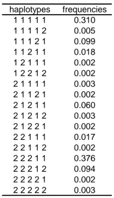
The performance of the MI algorithm was tested by simulations. Genotypes of case-parent trios were simulated at five completely linked loci under different genetic models with one or two disease susceptibility loci. The five loci were in linkage disequilibrium (LD) and the haplotype frequencies and resulting pattern of LD are shown in Table 1 and in supplementary information, Figure 1. Briefly the simulation process is the following: for each parent, two haplotypes are randomly picked from the population of 17 possible 5-locus haplotypes where each haplotype has a frequency as reported in Table 1. Then, one haplotype is randomly drawn from each parent to generate the child’s genotype and, based on the penetrance associated with this genotype, an affection status is generated for the child. If the affection status is "unaffected", the trio is discarded and the process is repeated until we obtain sufficient trios with an “affected” child. Finally, missing data are generated completely at random, that is to say with the same percentage of missing data on each of the five SNPs.

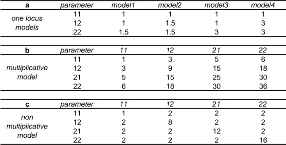
Concerning the genetic models, for one-locus models, the disease susceptibility (DS) locus was assumed to be the second marker (SNP2) and dominant or recessive models with genotype relative risks (GRR) of 1.5 or 3 were considered (see Table 2a). An additional model with no effect (GRR=1 for all genotypes) was also considered to evaluate the type I errors. For two-locus models, SNP2 and SNP3 were assumed to be the DS loci and both a multiplicative and non multiplicative models were considered (see Table 2). For each set of simulation, 500 simulated data sets were generated and run through the MI algorithm (with the following parameters: burn-in period = 1000 iterations, interval between two imputation n=1000 iterations and number of imputations m=9). For the different models, the power/type I error to detect the association was evaluated by determining, the proportion of replicates

among the 500 replicates where the combined p-value (as defined in equation 9) at SNP2 (assumed disease susceptibility site) was smaller than or equal to 5%. The performance of the algorithm for parameter estimation was also studied by reporting the bias and 95% CI

coverage for the different GRR estimations.

Results

Type I error rates for a nominal value of 5% are presented in Figure 1 for different levels of missing data. As expected, when families with missing data are ignored, we find that type I errors are not inflated by the presence of missing data, since these missing data are at random with respect to genotypes (see curve without MI). The use of the MI method does not increase the type I errors for up to 30% of missing data. Above 30%, we observe a significant increase in type I error rates. For 50% of missing data, there is a three fold increase in the type I error (0.16 instead of 0.05). This increase in the type I error rate can be explained by the fact that the number of families without missing data (complete families) becomes too small (for 50% missing data, less than one fourth of the families are complete, as shown in Figure 1) and in incomplete families, several genotypes might be missing. Under these circumstances, missing data are poorly inferred and the test becomes anti-conservative.

Figure 2 shows the power to detect association under the different one locus models. Without the MI algorithm, the power of detection of the DS site is sensitive to missing data due to the decrease of the sample size. The more the percentage of missing data increases, the more the number of informative families decreases and consequently, the more the power to detect the DS site decreases. In this context, the MI algorithm allows good power for detection of the DS site. For the recessive model (Figure 2a), we see a loss in power of 14.2% with 30% of missing data (without the MI algorithm, we observed a loss in power of 58% in the same configuration). For the dominant model (Figure 2b), the power remains at approximately 80% with 30% of missing data (so basically no loss in power as compared to a 59.1% power loss when MI algorithm is not used).

To check the efficiency of the MI method, the correlation between p-values obtained on the true complete data sets (available to us since this is simulated data) and p-values obtained by

using the MI algorithm on the same data, after adding a percentage of missing data, were investigated (supplementary information, Figure 2). With 5% missing data, we note a very good correlation rate in both models. With 50% of missing data, correlations are obviously lower: on the recessive model (model 1) p-values are often decreased and consequently a lot of non significant tests became significant. In contrary, p-values are slightly increased for the dominant model (model 2). Consequently, the efficiency of the MI is limited when the percentage of missing information is high; nevertheless, for up to 30% missing data this method gives acceptable performance.

We performed analysis to examine how often the DS site gives the highest score (i.e. the highest test statistic) as a function of the percentage of missing data (Figure 3). For the recessive model, we see a loss of detection of the true DS site of 14.4% with 30% missing data (without the MI algorithm, we observed a loss of detection of 33.8%). On the dominant model, we see a loss of detection of 0.2% with 30% missing data against a loss of detection of 30% without using the MI algorithm.

To investigate parameter estimation under the MI method, results with and without using the algorithm have been compared. With or without the MI algorithm, when the same percentage of missing data is used for all loci, no bias is expected. Without MI, when conditional logistic regression is used, only families genotyped for all markers are taken into account. So, missing data will involve a decrease in the sample size ( e.g. only 15% of informative families are available for analysis with 50% missing data) but not a change in the properties of the model. Table 1 of the supplementary information confirms this point: for each of the models

considered, the bias between the observed and the expected values of the genotype relative risks is near 0, and the 95% confidence intervals for the genotype relative risk parameters correctly cover the true values approximately 95% of the time (for a missing data proportion

of up to about 30%). We also investigated the correlation between the parameter estimates obtained from the true complete data set and those obtained using the MI approach

(supplementary information, Figure 3) and found that as expected the correlation decreases as the percentage of missing data increases but even with 50% of missing data, there is still a strong correlation.

Two 2-locus models have also been investigated. Figure 4 shows the bias between the expected and the observed haplotypic risks for different rates of missing data under the multiplicative model only, since risk estimation on haplotypes only have a sense if haplotypes have a multiplicative effect. For up to 10% of missing data, bias is weak with and without MI. For a larger percentage of missing data and when missing data are ignored, we observe a strong increase in the bias for all the haplotype relative risks. In contrast, when we use the MI algorithm, the bias stays reasonably low. For example, with 50% of missing data the bias is in the range [26.5 , 29.1] without MI compared to [0.15 , 1.17] with MI.

Figure 5 presents the bias obtained under the two models on phased genotypic risks. The median bias over the 10 genotype relative risks is reported. As for haplotypic risks, we note a high increase in the bias when the percentage of missing data increases. Without MI the median bias reaches 32.89 for the multiplicative model and 30.47 for the non multiplicative model opposed to a weak increase with MI (1.16 for the multiplicative model and 4.47 with the non multiplicative model). However, observed bias could be very different from one genotype to another and as expected, strong bias may be observed especially for rare genotypes.

These results confirm the ones obtained by Cordell [10] when using MI on case-control data. An important difference however between case-control and trio data is the fact that under a non-multiplicative model, the case-control data do not allow the distinction between the two following genotypes: the one composed by haplotypes aA and bB and the one composed by

haplotypes aB and bA. Indeed, use of an MI algorithm with case/control data [10]

distinguishes between these configurations by borrowing information (when it is possible) from resolvable genotypes under a Hardy Weinberg equilibrium assumption which

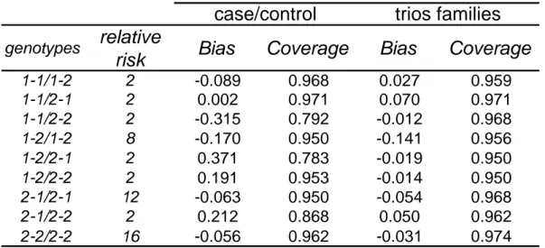
corresponds to assuming multiplicative haplotype effects. Consequently, this method fails for case/control data when the underlying haplotypic effects are not multiplicative [10]. However, with family data, information from the parents can allow knowledge of this phased genotype for the affected child. We performed simulations under different multiplicative and non-multiplicative models to check this property of the case/parent trio data. We choose to present in this paper results obtained with one of the non-multiplicative models used in [10] with 10 percent of missing data. Table 3 shows the bias and coverage when using the MI approach in a case/control and in a case/parent trio data set. As expected, we note the presence of a bias higher than 0.3 with the case/control data with poor confidence interval coverage (near 0.8) for both genotypes 1-1/2-2 and 1-2/2-1. The use of case/parent trio families generally gives less bias, particularly for the two phased genotypes (bias of 0.012 and 0.019 respectively). Consequently, we confirm the capacity of the method to correctly estimate these two phased genotype configurations with family data, which is not the case for case/control data.

Discussion

We have proposed an MI algorithm for testing and estimation of genotype and haplotype effects using case/parent trio data. Through simulations, we have examined the efficiency of the MI algorithm on several one and two locus models. Results show the usefulness of the MI approach With conditional logistic regression, this approach allows us to work with three pseudocontrols for each family whereas in the original case/pseudocontrol approach, only one pseudocontrol can be generated for families with unknown phase. When the percentage of missing data is small, parameter estimation can be correct without the use of MI.

Nevertheless, use of MI increases efficiency and allows better comparison of results at

different loci and detection of the true disease susceptibility site. Obviously, the MI algorithm is only one of the possible methods to take into account uncertainty due to missing data. The MI approach proposed here shares some similarities with Gibbs sampling and also with the stochastic EM algorithm [16-18]. Indeed, the sampling mechanism used in the IP algorithm that we describe is virtually identical to that used in Gibbs sampling. The main difference between MI and Gibbs sampling or an EM algorithm (either in its original or stochastic version) is that in a Gibbs sampling or EM algorithm framework, one runs the algorithm until convergence and uses the final parameter estimates obtained to make inference. In the MI approach, one instead writes out imputed data sets at intervals (e.g. every 1000 iterations), analyses these imputed data sets using standard statistical methods (e.g. regression) and then uses methods described in the MI literature [8,12,13] to produce a combined parameter estimate or make combined inference from all of the imputed data sets.

Compared to Gibbs sampling or an EM algorithm, MI is thus a two stage procedure. In the first stage one performs imputation to generate 3-10 imputed data sets; in the second stage one performs analysis on these imputed data sets and produces a combined result. The main advantage of this from an operational point of view is that one need not actually fit the full

model at the second stage. For instance, one could do the imputation assuming that 3 loci in a region influence disease, but then at the analysis stage one could fit the full model where all 3 loci influence disease, or one could fit a restricted model where just 2 of the loci influence disease, or indeed a further restricted model where just one of the loci influences disease. To compare all of these nested models in an EM or Gibbs sampling procedure, one would have to run the EM/Gibbs sampling algorithm 3 separate times, whereas in the MI approach one runs the IP algorithm only once, then fits the different nested models at the analysis stage.

Conceptually and in practice, therefore, it appears that MI is a promising approach for use in the search for disease susceptibility genes. Future work will involve extending this approach for association analysis using larger family structures (e.g. extended pedigrees) and with quantitative as opposed to merely dichotomous (disease) traits.

Acknowledgements

We thank Dr David Clayton for his help with multiple imputation algorithm. We also thank the REFGENSEP for sharing data. Support for this work was provided by the ARSEP.

References :

1 Spielman RS, McGinnis RE, Ewens WJ: Transmission test for linkage

disequilibrium: The insulin gene region and insulin-dependent diabetes mellitus (iddm). Am J Hum Genet 1993;52:506-516.

2 Cordell HJ, Clayton DG: A unified stepwise regression procedure for evaluating the relative effects of polymorphisms within a gene using case/control or family data: Application to hla in type 1 diabetes. Am J Hum Genet 2002;70:124-141.

3 Dudbridge F, Koeleman BP, Todd JA, Clayton DG: Unbiased application of the transmission/disequilibrium test to multilocus haplotypes. Am J Hum Genet

2000;66:2009-2012.

4 Dudbridge F: Pedigree disequilibrium tests for multilocus haplotypes. Genet Epidemiol 2003;25:115-121.

5 Horvath S, Xu X, Lake SL, Silverman EK, Weiss ST, Laird NM: Family-based tests for associating haplotypes with general phenotype data: Application to asthma genetics. Genet Epidemiol 2004;26:61-69.

6 Cordell HJ, Barratt BJ, Clayton DG: Case/pseudocontrol analysis in genetic association studies: A unified framework for detection of genotype and haplotype

associations, gene-gene and gene-environment interactions, and parent-of-origin effects. Genet Epidemiol 2004;26:167-185.

7 Schafer JL: Multiple imputation: A primer. Stat Methods Med Res 1999;8:3-15.

8 Schafer JL: Analysis of incomplete multivariate data. Chapman & Hall/CRC, 1997.

9 Little RJA, Rubin DB: Statistical analysis with missing data, ed 2nd ed. Wiley-interscience, 2002.

10 Cordell HJ: Estimation and testing of genotype and haplotype effects in case-control studies: Comparison of weighted regression and multiple imputation procedures. Genet Epidemiol 2006;30:259-275.

11 Tanner M, Wong W: The calculation of posterior distributions by data augmentation (with discussion). J Amer Stat Soc 1987;81:528-550.

12 Rubin DB: Multiple imputation for non reponse in surveys. New York, 1987. 13 Li K, Meng X, Raghunathan TE, Rubin DB: Significance levels from repeated p-values with multiply-imputed data. Statistica Sinica 1991;1:65-92.

14 Self SG, Longton G, Kopecky KJ, Liang KY: On estimating hla/disease association with application to a study of aplastic anemia. Biometrics 1991;47:53-61.

15 Schaid DJ: General score tests for associations of genetic markers with disease using cases and their parents. Genet Epidemiol 1996;13:423-449.

16 Tregouet DA, Escolano S, Tiret L, Mallet A, Golmard JL: A new algorithm for haplotype-based association analysis: The stochastic-em algorithm. Ann Hum Genet

2004;68:165-177.

17 Deltour I, Richardson S, Le Hesran JY: Stochastic algorithms for markov models estimation with intermittent missing data. Biometrics 1999;55:565-573.

18 Stephens M, Smith NJ, Donnelly P: A new statistical method for haplotype reconstruction from population data. Am J Hum Genet 2001;68:978-989.

19 Alizadeh M, Babron MC, Birebent B, Matsuda F, Quelvennec E, Liblau R, Cournu-Rebeix I, Momigliano-Richiardi P, Sequeiros J, Yaouanq J, Genin E, Vasilescu A, Bougerie H, Trojano M, Martins Silva B, Maciel P, Clerget-Darpoux F, Clanet M, Edan G, Fontaine B, Semana G: Genetic interaction of ctla-4 with hla-dr15 in multiple sclerosis patients. Ann Neurol 2003;54:119-122.

haplotypes frequencies 1 1 1 1 1 0.310 1 1 1 1 2 0.005 1 1 1 2 1 0.099 1 1 2 1 1 0.018 1 2 1 1 1 0.002 1 2 2 1 2 0.002 2 1 1 1 1 0.003 2 1 1 2 1 0.002 2 1 2 1 1 0.060 2 1 2 1 2 0.003 2 1 2 2 1 0.002 2 2 1 1 1 0.017 2 2 1 1 2 0.002 2 2 2 1 1 0.376 2 2 2 1 2 0.094 2 2 2 2 1 0.002 2 2 2 2 2 0.003

Table 1: Haplotype frequencies for the five loci considered in the simulations.

a parameter model1 model2 model3 model4 11 1 1 1 1 12 1 1.5 1 3 22 1.5 1.5 3 3 b parameter 11 12 21 22 11 1 3 5 6 12 3 9 15 18 21 5 15 25 30 22 6 18 30 36 c parameter 11 12 21 22 11 1 2 2 2 12 2 8 2 2 21 2 2 12 2 22 2 2 2 16 one locus models multiplicative model non multiplicative model

Table 2: a. List of the different 1-locus models used in simulation where parameters correspond to the genotype relative risks for genotypes 1/1, 1/2, 2/2 respectively.

b. Multiplicative 2-locus model where parameters correspond to the genotype relative risk arising from the association of the two transmitted haplotypes, with the four possible haplotypes denoted 11, 12, 21, 22 respectively .

c. Non-multiplicative 2-locus model where parameters correspond to the genotype relative risk arising from the association of the two transmitted haplotypes, with the four possible haplotypes denoted 11, 12, 21, 22 respectively.

genotypes

relative

risk

Bias

Coverage

Bias

Coverage

1-1/1-2 2 -0.089 0.968 0.027 0.959 1-1/2-1 2 0.002 0.971 0.070 0.971 1-1/2-2 2 -0.315 0.792 -0.012 0.968 1-2/1-2 8 -0.170 0.950 -0.141 0.956 1-2/2-1 2 0.371 0.783 -0.019 0.950 1-2/2-2 2 0.191 0.953 -0.014 0.950 2-1/2-1 12 -0.063 0.950 -0.054 0.968 2-1/2-2 2 0.212 0.868 0.050 0.962 2-2/2-2 16 -0.056 0.962 -0.031 0.974

case/control

trios families

Table 3: Bias and 95% confidence interval coverage of genetic parameter estimates from two-locus simulation study when using case/control or case/parent trio data with 10% missing data. The second column corresponds to the expected relative risk associated with each genotype.

Figure Legend :

Figure 1: Type 1 error at α=0.05 on simulated data as a function of the percentage of missing data when using or not the MI approach. The number of complete families available for the study without MI is plotted on the second y axis.

Figure 2: Power at α=0.05 on simulated data as a function of the percentage of missing data when using or not the MI approach for a recessive model (a) and a dominant model (b) with genotype relatve risks 1.5. The number of complete families available for the study without MI is plotted on the second y axis.

Figure 3: Percentage of replicates among the 500 replicates where the disease susceptibility site (locus 2) gives the best score in function of the percentage of missing data when using or not the MI approach for a recessive (a) and a dominant model (b) with genotype relative risks 1.5.

Figure 4: haplotypic bias between the expected and the observed haplotypic relative risk in function of the percentage of missing data in the case of the 2-locus multiplicative model when using or not the MI algorithm. Haplotype relative risks hr2, hr3 and hr4 correspond to the relative risks for haplotypes 12, 21 and 22 respectively (relative to haplotype 11).

Figure 5: Median of the absolute genotypic bias in function of the percentage of missing data in the case of the 2-locus multiplicative and non multiplicative model when using or not MI algorithm.

0 0.05 0.1 0.15 0.2 0% 10% 20% 30% 40% 50% % of missing data ty pe 1 er ro r 0 125 250 375 500 n

umber of complete familie

s with MI without MI number of complete families Figure 1

a.

recessive model

0 0.2 0.4 0.6 0.8 1 0% 10% 20% 30% 40% 50% % of missing data po wer 0 100 200 300 400 500 nu m b e r of c o m p le te f a m ili es with MI without MI number of complete families b.

dominant model

0 0.2 0.4 0.6 0.8 1 0% 10% 20% 30% 40% 50% % of missing data power 0 100 200 300 400 500 number of complet e families _{with MI} without MI number of complete families Figure 2

a.

b.

Figure 3

0 5 10 15 20 25 30 0% 10% 20% 30% 40% 50% % of missing data bias hr2 with MI hr3 with MI hr4 with MI hr2 hr3 hr4 Figure 4

0 5 10 15 20 25 30 35 0% 1% 5% 10% 20% 30% 40% 50% % of missing data me dian bias mult with MI non mult with MI mult without MI non mult without MI

Figure 5

Supplementary information: model 1 expected 0% 1% 5% 10% 20% 30% 40% 50% 500 486.364 434.362 374.658 271.916 189.814 125.752 77.82 GRR2 1 0.006 0.006 0.007 0.008 0.008 0.001 0.010 0.040 GRR3 1.5 0.007 0.006 0.006 0.006 0.007 -0.009 -0.005 0.053 coverage 2 0.95 0.938 0.940 0.930 0.946 0.936 0.942 0.966 0.960 coverage 3 0.95 0.928 0.924 0.926 0.940 0.948 0.958 0.954 0.966 GRR2 1 0.006 0.007 0.012 0.018 0.033 0.055 0.096 0.154 GRR3 1.5 0.007 0.008 0.013 0.015 0.022 0.027 0.036 0.045 coverage 2 0.95 0.938 0.936 0.938 0.934 0.928 0.932 0.906 0.843 coverage 3 0.95 0.928 0.928 0.936 0.936 0.928 0.922 0.926 0.896 model 2 expected 0% 1% 5% 10% 20% 30% 40% 50% 500 486.162 434.33 374.626 272.086 189.468 125.198 78.422 GRR2 1.5 0.008 0.007 0.010 0.014 0.017 0.019 0.015 0.008 GRR3 1.5 -0.001 -0.002 0.000 0.006 0.004 0.006 -0.006 0.000 coverage 2 0.95 0.960 0.958 0.960 0.956 0.952 0.962 0.976 0.958 coverage 3 0.95 0.962 0.952 0.958 0.960 0.952 0.948 0.962 0.952 GRR2 1.5 0.008 0.009 0.014 0.020 0.036 0.054 0.084 0.129 GRR3 1.5 -0.001 0.001 0.006 0.012 0.017 0.023 0.021 0.018 coverage 2 0.95 0.960 0.954 0.952 0.952 0.950 0.948 0.942 0.910 coverage 3 0.95 0.962 0.958 0.954 0.968 0.958 0.960 0.928 0.938 model 3 expected 0% 1% 5% 10% 20% 30% 40% 50% 500 486.654 434.302 374.572 271.576 188.566 126.432 77.568 GRR2 1.5 0.009 0.008 0.007 0.007 0.015 0.016 0.001 0.045 GRR3 1.5 0.003 0.002 0.004 0.005 0.011 0.014 0.023 0.096 coverage 2 0.95 0.922 0.924 0.912 0.938 0.940 0.942 0.932 0.964 coverage 3 0.95 0.934 0.930 0.932 0.930 0.938 0.940 0.940 0.954 GRR2 1.5 0.009 0.010 0.015 0.023 0.040 0.068 0.116 0.179 GRR3 1.5 0.003 0.005 0.009 0.015 0.022 0.032 0.049 0.058 coverage 2 0.95 0.922 0.920 0.916 0.922 0.924 0.918 0.898 0.830 coverage 3 0.95 0.934 0.934 0.938 0.936 0.924 0.930 0.922 0.904 model 4 expected 0% 1% 5% 10% 20% 30% 40% 50% 500 486.066 433.57 375.192 272.884 189.626 125.612 78.068 GRR2 1.5 0.012 0.013 0.009 0.016 0.017 0.039 0.070 0.285 GRR3 1.5 -0.002 0.000 -0.007 -0.001 0.006 0.010 0.056 0.247 coverage 2 0.95 0.946 0.958 0.962 0.974 0.956 0.942 0.950 0.966 coverage 3 0.95 0.958 0.956 0.956 0.956 0.960 0.970 0.968 0.952 GRR2 1.5 0.012 0.014 0.016 0.025 0.036 0.050 0.084 0.137 GRR3 1.5 -0.002 0.000 0.003 0.010 0.014 0.008 0.015 0.033 coverage 2 0.95 0.946 0.944 0.954 0.954 0.964 0.956 0.948 0.922 coverage 3 0.95 0.958 0.954 0.964 0.960 0.970 0.958 0.948 0.934 without multiple imputation with multiple imputation % of missing data % of missing data number of complete families % of missing data with multiple imputation % of missing data without multiple imputation number of complete families without multiple imputation number of complete families with multiple imputation without multiple imputation number of complete families with multiple imputation

Supplementary table 1: Bias and coverage of genetic parameter estimates from one-locus simulation study as a function of the percentage of missing data. The number of informative families for the analysis without MI is noted on the third row.

Supplementary Figure 1: LD pattern between the five loci considered in the simulations. Gradation of greys represents the level of the D’ and numbers are the D’ values. This LD pattern is similar to the one observed in the CTLA4 gene in a sample of 450 multiple sclerosis trios [19].

Supplementary Figure 2: Correlation plot between the logarithm of the p-value obtained on the complete data file and data with 5, 30 and 50% of missing data when using MI approach on the recessive model 1 (a, b and c respectively) and the dominant model 2 (d, e and f) with genotype relative risks 1.5. For a better understanding of these graphs, the linear equation y=x has been plotted.

Supplementary Figure 3: Correlation plot between the genotype relative risk of the

homozygous 2/2 obtained on the complete data file and data with 5, 30 and 50% of missing data when using MI approach on the recessive model 1 (a, b and c respectively) and the dominant model 2 (d, e and f) with genotype relative risk 1.5. For a better understanding of these graph, the linear equation y=x has been plotted.

Supplementary information, figure1

a. d. recessive model 0 5 10 15 20 0 5 10 15 20

-ln(p with complete data file)

-l n(p _ v a lue wit h 5% o f MD) dominant model 0 5 10 15 20 0 5 10 15 20

-ln(p with complete data file)

-l n(p _ v a lue wit h 5% o f MD) b. e. recessive model 0 5 10 15 20 0 5 10 15 20

-ln(p with complete data file)

-ln( p_v alu e wi th 30 % of MD) dominant model 0 5 10 15 20 0 5 10 15 20

-ln(p with complete data file)

-ln( p_v alu e wi th 30 % of MD) c. f. recessive model 0 5 10 15 20 0 5 10 15 20

-ln(p with complete data file)

-ln( p_v alu e wi th 50 % of MD) dominant model 0 5 10 15 20 0 5 10 15 20

-ln(p with complete data file)

-l n( p _ v a lu e w it h 50 % of M D )

Supplementary information, figure 2

a d recessive model -0.2 0 0.2 0.4 0.6 0.8 1 1.2 -0.2 0 0.2 0.4 0.6 0.8 1 1.2

GRR2 on complete data file

GR R 2 on da ta w it h 5% o f M D 3 dominant model -0.2 0 0.2 0.4 0.6 0.8 1 1.2 -0.2 0 0.2 0.4 0.6 0.8 1 1.2

GRR2 on complete data file

GR R 2 on da ta w it h 5% o f M D b e recessive model -0.2 0 0.2 0.4 0.6 0.8 1 1.2 -0.2 0 0.2 0.4 0.6 0.8 1 1.2

GRR2 on complete data file

GR R 2 on da ta w it h 30 % of M D dominant model -0.2 0 0.2 0.4 0.6 0.8 1 1.2 -0.2 0 0.2 0.4 0.6 0.8 1 1.2

GRR2 on complete data file

GR R 2 on da ta w it h 30 % of M D c f recessive model -0.2 0 0.2 0.4 0.6 0.8 1 1.2 -0.2 0 0.2 0.4 0.6 0.8 1 1.2

GRR2 on complete data file

GRR 2 o n dat a wit h 50% of MD dominant model -0.2 0 0.2 0.4 0.6 0.8 1 1.2 -0.2 0 0.2 0.4 0.6 0.8 1 1.2

GRR2 on complete data file

GRR2 o n dat a wit h 5 0% of MD

Supplementary information, figure 3