Testing the effect of the rock record
on diversity: a multidisciplinary approach
to elucidating the generic richness
of sauropodomorph dinosaurs through time
Philip D. Mannion
1∗, Paul Upchurch
1, Matthew T. Carrano
2and Paul M. Barrett
3 1Department of Earth Sciences, University College London, Gower Street, London, WC1E 6BT, UK2Department of Paleobiology, National Museum of Natural History, Smithsonian Institution, P.O. Box 37012, Washington, DC 20013-7012, USA
3Department of Palaeontology, The Natural History Museum, Cromwell Road, London, SW7 5BD, UK
(Received 07 October 2009; revised 24 March 2010; accepted 29 March 2010)
ABSTRACT
The accurate reconstruction of palaeobiodiversity patterns is central to a detailed understanding of the macroevolutionary history of a group of organisms. However, there is increasing evidence that diversity patterns observed directly from the fossil record are strongly influenced by fluctuations in the quality of our sampling of the rock record; thus, any patterns we see may reflect sampling biases, rather than genuine biological signals. Previous dinosaur diversity studies have suggested that fluctuations in sauropodomorph palaeobiodiversity reflect genuine biological signals, in comparison to theropods and ornithischians whose diversity seems to be largely controlled by the rock record. Most previous diversity analyses that have attempted to take into account the effects of sampling biases have used only a single method or proxy: here we use a number of techniques in order to elucidate diversity. A global database of all known sauropodomorph body fossil occurrences (2024) was constructed. A taxic diversity curve for all valid sauropodomorph genera was extracted from this database and compared statistically with several sampling proxies (rock outcrop area and dinosaur-bearing formations and collections), each of which captures a different aspect of fossil record sampling. Phylogenetic diversity estimates, residuals and sample-based rarefaction (including the first attempt to capture ‘cryptic’ diversity in dinosaurs) were implemented to investigate further the effects of sampling. After ‘removal’ of biases, sauropodomorph diversity appears to be genuinely high in the Norian, Pliensbachian–Toarcian, Bathonian–Callovian and Kimmeridgian–Tithonian (with a small peak in the Aptian), whereas low diversity levels are recorded for the Oxfordian and Berriasian–Barremian, with the Jurassic/Cretaceous boundary seemingly representing a real diversity trough. Observed diversity in the remaining Triassic–Jurassic stages appears to be largely driven by sampling effort. Late Cretaceous diversity is difficult to elucidate and it is possible that this interval remains relatively under-sampled. Despite its distortion by sampling biases, much of sauropodomorph palaeobiodiversity can be interpreted as a reflection of genuine biological signals, and fluctuations in sea level may account for some of these diversity patterns.
Key words: dinosaurs, diversity, extinction, macroevolution, rarefaction, residuals, rock record, sampling bias,
sauropodomorphs, sea level. CONTENTS
I. Introduction . . . . 2 (1) Previous studies of dinosaur diversity . . . . 3 (2) Sauropodomorph diversity . . . . 6 * Address for correspondence: (Tel:+44 020 7679 30165; E-mail: [email protected]).
II. Materials and methods . . . . 7
(1) Data . . . . 7
(2) Diversity estimates . . . . 7
(a) Introduction . . . . 7
(b) Fit of sauropodomorph phylogenies to stratigraphy . . . . 7
(c) Taxonomic units of analysis . . . . 8
(d) Geological age of taxa . . . . 8
(3) Preservational biases and sampling quality . . . . 9
(a) Rock outcrop . . . . 10
(b) Collecting effort . . . . 10
(c) Residuals . . . . 10
(d) Rarefaction . . . . 11
(4) Comparisons with sea level . . . . 12
(5) ‘Summary’ diversity . . . . 12
III. Analyses and results . . . . 12
(1) Sauropodomorph taxic diversity . . . . 12
(2) Statistical comparisons between phylogenetic and taxic diversity . . . . 12
(3) Statistical comparisons between diversity and sampling proxies . . . . 13
(4) Residuals and rarefaction . . . . 15
(5) Historical collecting effort . . . . 16
(6) Comparisons between sea level and diversity . . . . 16
IV. Discussion . . . . 17
(1) ‘Summary’ diversity through time . . . . 17
(a) Late Triassic . . . . 17
(b) Early Jurassic . . . . 17
(c) Middle Jurassic . . . . 17
(d) Late Jurassic . . . . 17
(e) Early Cretaceous . . . . 17
(f ) Late Cretaceous . . . . 18
(2) Does our choice of phylogeny make a difference? . . . . 18
(3) Did sea level control sauropodomorph diversity? . . . . 19
(4) Good rock record versus poor fossil dating . . . . 20
(5) Methodological choices . . . . 20
(a) Different approaches to correcting diversity . . . . 20
(b) Time-slicing . . . . 20
V. Conclusions . . . . 21
VI. Acknowledgements . . . . 22
VII. References . . . . 22
VIII. Supporting Information . . . . 27
I. INTRODUCTION
Deducing diversity patterns through time is an important element in understanding the macroevolutionary history of a group of organisms. The recovery of peaks and troughs in the diversity curve, and knowledge of their magnitude and sequence, enables us to assess the tempo and mode of evolution in any clade, as well as recognise major events in the history of life, including adaptive radiations and extinctions (Valentine, 1985; Jablonski, Erwin & Lipps, 1996; Jablonski, 2005). In addition, detailed knowledge of these patterns allows testing of potentially important evolutionary processes, such as competition and co-evolution, over extended temporal scales (e.g. Bakker, 1978; Vermeij, 1983; Collinson & Hooker, 1991; Benton, 1996; Barrett & Upchurch, 2005; Butler et al., 2009a, b, c). There are several ways in which palaeobiodiversity can
be defined and thus measured (Smith, 1994); here, we use ‘diversity’ in the sense of taxonomic richness (e.g. the number of species, genera, etc. that occur during a given time period). The study of dinosaur diversity has proved to be a fruitful, yet controversial, area of research into Mesozoic palaeobiodiversity patterns (Dodson, 1990; Haubold, 1990; Dodson & Dawson, 1991; Sereno, 1997, 1999; Fastovsky
et al., 2004; Taylor, 2006; Wang & Dodson, 2006; Carrano,
2008a; Lloyd et al., 2008; Barrett, McGowan & Page, 2009). There have also been several analyses investigating the diversity of particular clades within Dinosauria (Hunt
et al., 1994; Lockley et al., 1994; Weishampel & Jianu,
2000; Barrett & Willis, 2001; Barrett & Upchurch, 2005; Upchurch & Barrett, 2005; Mannion, 2009b). The majority of these studies were based on taxonomic diversity records (i.e. direct readings of the fossil record by counting the numbers of genera or families that can be observed through
geological time). Seven of these analyses (Sereno, 1997, 1999; Weishampel & Jianu, 2000; Upchurch & Barrett, 2005; Lloyd et al., 2008; Barrett et al., 2009; Mannion, 2009b) incorporated phylogenetic relationships into the diversity estimates. A second subset of studies (Fastovsky et al., 2004; Barrett & Upchurch, 2005; Upchurch & Barrett, 2005; Wang & Dodson, 2006; Carrano, 2008a; Lloyd et al., 2008; Barrett et al., 2009; Mannion, 2009b; Mannion & Upchurch, 2010b) have attempted to take into account sampling biases that might affect any reading of the dinosaur fossil record. However, each of these analyses utilised only a subset of the available techniques for elucidating diversity patterns, making it unclear how the results would have differed if alternative methods had been applied; consequently, there are few examples where we can compare the performances of different methods side-by-side.
Herein, we present the results of a multi-method approach to the identification and removal of sampling biases in palaeodiversity analyses. We utilise a recently developed and virtually comprehensive dataset to analyse sauropodomorph dinosaur palaeodiversity using the full spectrum of competing techniques. This paper builds on previous sauropodomorph diversity analyses, particularly those of Upchurch & Barrett (2005) and Barrett et al. (2009). A taxic diversity estimate for all valid sauropodomorph taxa and several competing phylogenies are plotted onto stratigraphic range charts in order to produce and compare diversity curves. We investigate a number of preservational biases potentially affecting sauropodomorph diversity using a variety of
methods (including residuals and rarefaction), and examine whether peaks and troughs in diversity correlate with potential causal factors such as sea level.
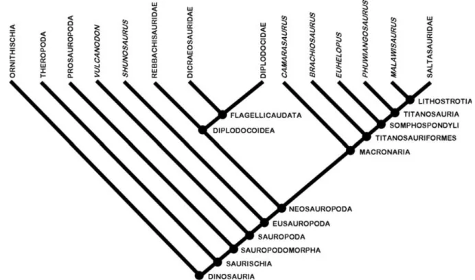
Sauropodomorpha is the sister group of Theropoda, which together comprise the Saurischia (Fig. 1; Weishampel, Dodson & Osm´olska, 2004b, and references therein). Several aspects of these large-bodied herbivores make them particularly suitable for examining and testing long-term diversity patterns. First, sauropodomorph remains have been found on all continents and by the Middle Jurassic, at the latest, they had achieved a global distribution (McIntosh, 1990; Upchurch, 1995; Wilson & Sereno, 1998; Upchurch, Hunn & Norman, 2002; Upchurch, Barrett & Dodson, 2004; Weishampel et al., 2004a). Second, they were a significant and diverse part of Mesozoic terrestrial ecosystems (Fig. 2) until their extinction at the end of the Cretaceous along with the other non-avian dinosaurs; this evolutionary history spans 160 million years (Myr). Finally, the clade includes the largest terrestrial animals of all time (Wilson, 2002; Upchurch et al., 2004), with Argentinosaurus (body mass exceeding 70 tonnes; Mazzetta, Christiansen & Fari ˜na, 2004) a notable example, and as such has a high preservation potential.
(1) Previous studies of dinosaur diversity
The earliest modern studies of dinosaur diversity focused on determining the raw numbers of dinosaur taxa present during the Mesozoic (Dodson, 1990; Haubold, 1990). These analyses agreed on a general pattern that included three
Fig. 1. Simplified cladogram showing dinosaur inter-relationships, the main sauropodomorph lineages, and the stem- and
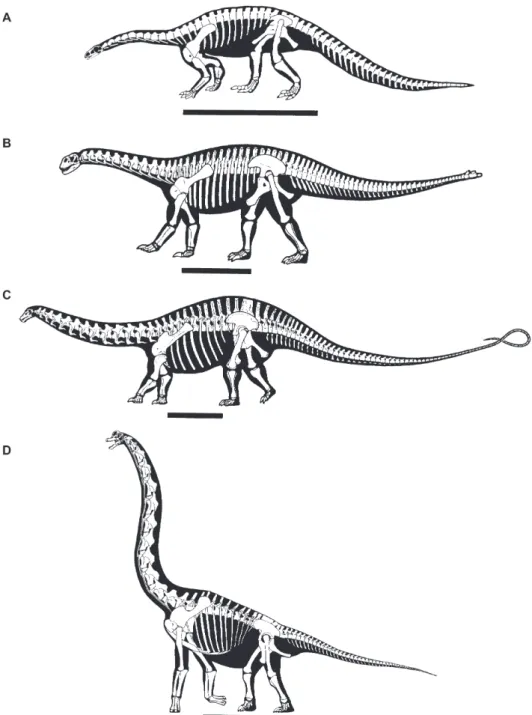
Fig. 2. Skeletal outlines of four sauropodomorphs: (A) Plateosaurus, (B) Shunosaurus, (C) Apatosaurus, (D) Brachiosaurus (after Wilson &
Sereno, 1998; Galton & Upchurch, 2004a; Upchurch et al., 2004). Scale bars= 2 m.
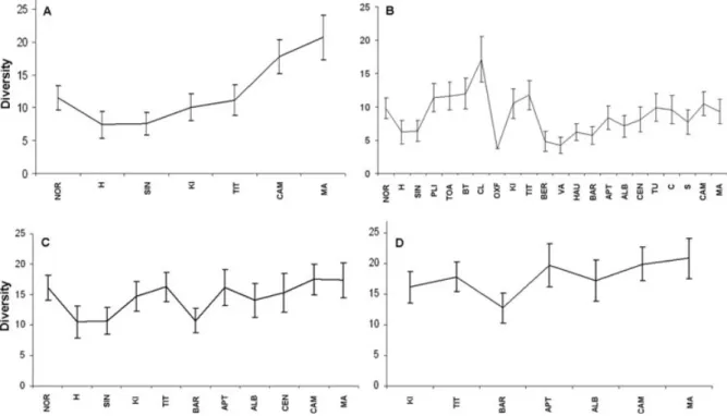
diversity peaks (Late Triassic, Late Jurassic and Late Cretaceous; Fig. 3A), which were suggested to be at least partly tied to sea level cycles; however, they presented opposing views on the specific relationships between diversity and sea level. Both studies acknowledged the importance of sampling and other biases, but were unable to assess them quantitatively.
Sereno (1997, 1999) produced time-calibrated cladograms for all dinosaurs and used these to assess diversity. This early attempt to assess phylogenetic diversity confirmed that the appearance of basal ornithischians (heterodontosaurids)
and basal sauropodomorphs (‘prosauropods’) in the Late Triassic resulted in a small diversity peak, with sauropod diversity reaching its apex in the Late Jurassic (Fig. 3B). Overall, dinosaur diversity was low in the earliest Cretaceous, followed by a general increase in the mid-Cretaceous and a large rise during the Campanian–Maastrichtian (83.5–65.5 Myr; Fig. 3B): ceratopsians and ornithopods achieved their greatest diversity at this time (Sereno, 1999). Although these two studies (Sereno, 1997, 1999) took into account the effects of available rock outcrop area on diversity, peaks were considered as genuine biological events, whereas troughs in
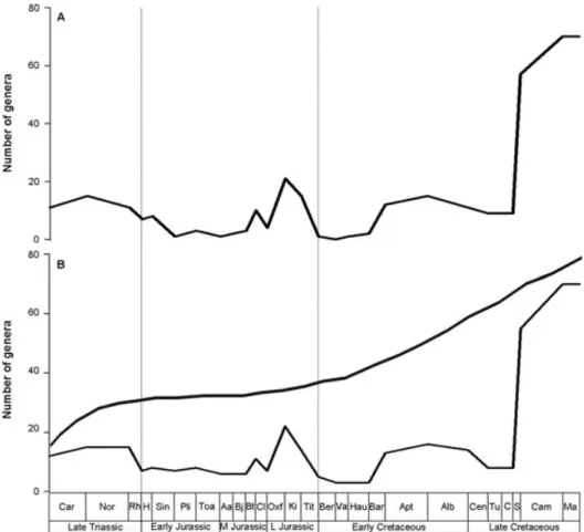
Fig. 3. Summary dinosaur diversity curves based on counts of numbers of genera through time: (A) modified from Dodson (1990);
(B) modified from Sereno (1999). The upper curve in B represents an estimated curve of diversity after taking into account available
outcrop area (after Sereno, 1999). Abbreviations: Car = Carnian, Nor = Norian, Rh = Rhaetian, H = Hettangian, Sin =
Sinemurian, Pli = Pliensbachian, Toa = Toarcian, Aa = Aalenian, Bj = Bajocian, Bt = Bathonian, Cl = Callovian, Oxf =
Oxfordian, Ki= Kimmeridgian, Tit = Tithonian, Ber = Berriasian, Va = Valanginian, Hau = Hauterivian, Bar = Barremian,
Apt= Aptian, Alb = Albian, Cen = Cenomanian, Tu = Turonian, C = Coniacian, S = Santonian, Cam = Campanian, Ma =
Maastrichtian.
diversity were interpreted as sampling biases. Consequently, the resultant estimated diversity curve showed a gradual diversity increase during the Triassic–Jurassic, before a relatively rapid increase throughout the Cretaceous (Fig. 3B). A similar pattern was recovered by Lloyd et al. (2008), who constructed a time-calibrated dinosaurian supertree which was used to estimate diversification rates across the clade. Several subsequent studies focused on estimating diversity patterns for individual clades of dinosaurs (e.g. Weishampel & Jianu, 2000; Barrett & Willis, 2001), whereas others attempted to investigate biotic turnover immediately prior to the end-Cretaceous extinction (e.g. Fastovsky et al., 2004; Wang & Dodson, 2006; Carrano, 2008a).
More recently, several workers have begun to address explicitly how biases in sampling, phylogeny and the fossil record might impact perceptions of dinosaur diversity. Barrett et al. (2009) assessed dinosaur diversity (including Mesozoic birds) based on taxic and phylogenetic curves for genera and species. In order to test whether geological sampling biases impacted the shapes of these curves, these authors constructed a diversity model utilising the
residuals method of Smith & McGowan (2007; see Section II). This model predicted the expected genus richness for each dinosaur clade using the number of dinosaur-bearing formations (DBFs) (see Table 1 for a summary of abbreviations used herein) present in each time interval as a geological proxy for the amount of dinosaur-bearing rock available through time (cf. Peters & Foote, 2001). Statistical comparisons between these models and the observed diversity curves suggested that ornithischian and theropod diversity patterns were significantly correlated with fluctuations in the rock record [as also suggested by Weishampel & Jianu (2000) and Upchurch & Barrett (2005)]. However, sauropodomorph diversity was largely independent of changes in the number of DBFs, potentially reflecting genuine evolutionary events (Barrett et al., 2009; see also Upchurch & Barrett, 2005). These results suggest that it may be possible to analyse and interpret certain genuine biological aspects of sauropodomorph diversification. Below we outline the current consensus view on sauropodomorph diversity before presenting a more detailed investigation into the effects of sampling on the genus richness of this clade.
Table 1. List of abbreviations used in the text
Abbreviation Definition
BPDE Barrett et al. (2009) phylogenetic diversity estimate BTDE Barrett et al. (2009) taxic diversity estimate DBCs Dinosaur-bearing collections
DBFs Dinosaur-bearing formations
LPDE Lloyd et al. (2008) phylogenetic diversity estimate MDE Modelled diversity estimate
Myr Million years
NOOs Numbers of opportunities to observe PDE Phylogenetic diversity estimate TDE Taxic diversity estimate TDEP Pruned taxic diversity estimate
TDEWE Western European taxic diversity estimate
UPDE Upchurch et al. (2004, 2007) phylogenetic diversity estimate
WPDE Wilson (2002) phylogenetic diversity estimate YPDE Yates (2007) phylogenetic diversity estimate
(2) Sauropodomorph diversity
The earliest known sauropodomorphs are Saturnalia and
Panphagia from the early Carnian (228 Myr; Late Triassic)
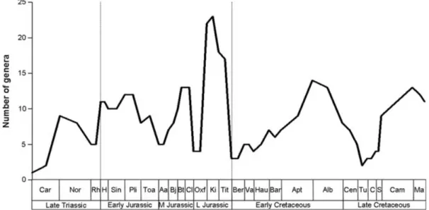
of Brazil and Argentina, respectively (Langer et al., 1999; Martinez & Alcober, 2009). An earlier record from the Middle Triassic of Madagascar (Flynn et al., 1999) has since been shown to represent a non-dinosaurian archosauromorph (Flynn et al., 2008). An early diversity peak comprised of basal sauropodomorphs and ‘prosauropods’ (e.g. Thecodontosaurus, Mussaurus and Plateosaurus) in the Norian (216.5–203.6 Myr; Late Triassic) was followed by a drop in the Rhaetian (203.6–199.6 Myr), before a prominent Early Jurassic increase (Fig. 4; Weishampel & Jianu, 2000; Barrett & Upchurch, 2005; Barrett et al., 2009). Non-eusauropod sauropodomorphs (including ‘prosauropods’; Fig. 1) became extinct prior to the Middle Jurassic, coincident with the
onset of a eusauropod radiation (Sereno, 1999; Barrett & Upchurch, 2005). Note that these taxa became extinct regardless of whether they are considered monophyletic (e.g. Gauthier, 1986; Benton et al., 2000; Galton & Upchurch, 2004a; Upchurch, Barrett & Galton, 2007) or a paraphyletic assemblage (Yates, 2003, 2004, 2007; Yates & Kitching, 2003); only the nature of this extinction may in some respects be a taxonomic artefact (see Forey et al., 2004).
Several studies have noted a Middle Jurassic peak in sauropod diversity (Hunt et al., 1994; Barrett & Willis, 2001; Upchurch & Barrett, 2005), which may reflect a neosauropod radiation (Wilson & Sereno, 1998; Figs 1, 4). The Oxfordian (161.2–155.7 Myr; early Late Jurassic) represents an apparent diversity trough (Upchurch & Barrett, 2005; Barrett et al., 2009), while the remaining Late Jurassic stages (Kimmeridgian-Tithonian; 155.7–145.5 Myr) are typically thought to have represented the highest peak in diversity (Fig. 4) (Bakker, 1977, 1978; Horner, 1983; Weishampel & Horner, 1987; Haubold, 1990; Hunt et al., 1994; Upchurch, 1995; Sereno, 1997, 1999; Wilson & Sereno, 1998; Weishampel & Jianu, 2000; Barrett & Willis, 2001; Upchurch & Barrett, 2005; Barrett et al., 2009), exemplified by well-known taxa such as Brachiosaurus and Diplodocus.
A prominent decline in the number of genera across the Jurassic/Cretaceous (J/K) boundary (145.5 Myr) is implied by the apparently reduced species richness of the earliest Cretaceous (Fig. 4) (Hunt et al., 1994; Wilson & Sereno, 1998; Upchurch & Barrett, 2005; Barrett et al., 2009). Sauropods underwent a major diversification in the mid-Cretaceous (Fig. 4), with this radiation predominantly composed of titanosaurs (Salgado, Coria & Calvo, 1997; Wilson & Upchurch, 2003; Curry Rogers, 2005; Upchurch & Barrett, 2005; Lloyd et al., 2008), as well as a small contribution from rebbachisaurid diplodocoids (Upchurch & Barrett, 2005; Sereno et al., 2007; Mannion, 2009a) (Fig. 1). Diversity apparently dropped in the mid-Late Cretaceous before
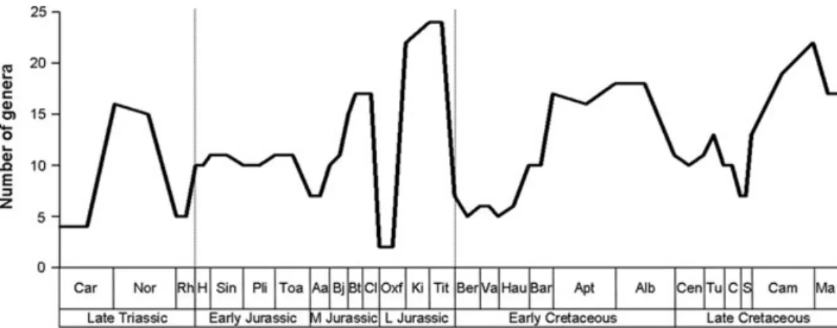
Fig. 4. Consensus of sauropodomorph diversity based primarily upon Upchurch & Barrett (2005) and Barrett et al. (2009). See
reaching another peak in the Campanian–Maastrichtian (83.5–65.5 Myr; Hunt et al., 1994; Weishampel & Jianu, 2000; Barrett & Willis, 2001; Upchurch & Barrett, 2005), although this peak is smaller than that in the Late Jurassic. There is also evidence for a decline in sauropod diversity prior to their final extinction at the Cretaceous/Paleogene (K/P) boundary (65.5 Myr; Fig. 4) (Upchurch & Barrett, 2005).
A number of these diversity peaks and troughs have been noted as corresponding with rises and falls in sea level (Haubold, 1990; Hunt et al., 1994; Upchurch & Barrett, 2005) and it has been suggested that some of these intervals, at least, may potentially represent genuine (i.e. biotic) diversity signals rather than purely the effects of taphonomic biases (Upchurch & Barrett, 2005; Barrett et al., 2009).
II. MATERIALS AND METHODS (1) Data
A global database of all known sauropodomorph body fossil occurrences was constructed, consisting of 2024 individuals (available as online Appendix). These data were collected primarily from the literature (including Weishampel et al., 2004a, b), supplemented with data from The Paleobiology
Database (www.paleodb.org; Carrano, 2008b) and personal
observations during museum visits (see online Appendix). The minimum number of individuals was estimated for each discrete geographic locality and stratigraphic level (see Mannion & Upchurch, 2010a). A compilation of all valid sauropodomorph taxa (175, as of September 2008) was extracted from this database (see online Appendix), based on updates made to Galton & Upchurch (2004a) and Upchurch
et al. (2004). The phylogenies of Wilson (2002), Upchurch et al. (2004, 2007), Yates (2007) and Lloyd et al. (2008) have
all been utilised.
(2) Diversity estimates
(a) Introduction
There are two main methods for measuring diversity. First, the ‘taxic’ approach (Levinton, 1988) defines the total geological range of each taxon and sums the numbers of taxa present in each time interval to produce a diversity curve. This approach has the benefits of: (1) allowing all taxa to be incorporated, (2) being computationally simple to implement and (3) not requiring knowledge of detailed phylogenetic relationships. However, the taxic method has been strongly criticised for its reliance on what is often considered an incomplete and biased fossil record, leading to the development of a second method, the phylogenetic approach (Novacek & Norell, 1982; Norell & Novacek, 1992a, b; Smith, 1994). This method calibrates the phylogenetic relationships between taxa against stratigraphy. It follows the bifurcation model of speciation (Hennig, 1965) in that sister taxa must have equal first appearance times; thus, the first appearance times of taxa are extended back in time to that of the oldest
known sister taxon occurrence, creating ‘ghost’ lineages or ranges, which reflect gaps in the fossil record (Norell, 1992, 1993). There are several criticisms of the phylogenetic method, however. For example, by only correcting for the first appearance times of taxa (i.e. through ‘ghost’ lineages), the phylogenetic method introduces an asymmetrical bias by not also extending extinction times forwards (Wagner, 1995, 2000b; Foote, 1996). Additionally, the assumption that ancestral taxa are rarely found in the fossil record (Lane, Janis & Sepkoski, 2005) means that they are absent among the terminal taxa of a phylogeny (Benton & Storrs, 1994). Also, when misdiagnosed ancestors are included in phylogenies, the addition of ghost lineages may over-inflate diversity estimates (Lane et al., 2005).
The use of the taxic approach has not been abandoned: many workers have utilised enhanced statistical techniques in attempts to resolve its problems (e.g. Alroy et al., 2008). Thus, both the taxic and phylogenetic methods have been applied here; through this pluralistic approach we hope to overcome the disadvantages of both methods (Wagner, 1995; Foote, 1996; Lane et al., 2005; Upchurch & Barrett, 2005). (b) Fit of sauropodomorph phylogenies to stratigraphy
Before we use phylogenies to reconstruct diversity, we need to have some idea of how well they fit stratigraphy in order to see how closely they sample and reflect the fossil record. Phylogenies are generally obtained solely from biological data and are usually independent of temporal information (Norell, 1996). Thus, by mapping cladograms onto stratigraphic range charts we can combine two independent methods for understanding the evolution of a group of organisms (see Pol & Norell, 2006, and references therein). Most dinosaur datasets have been demonstrated to show extremely high congruence between phylogeny and stratigraphy (Brochu & Norell, 2000; Wilson, 2002; Rauhut, 2003; Pol & Norell, 2006; Wills, Barrett & Heathcote, 2008), leading Wills et al. (2008) to comment that our knowledge of the dinosaur fossil record is more than adequate for investigating temporal patterns of dinosaur diversity. Regions of diversity curves where different phylogenies produce comparable results may represent better constrained time periods, whereas incompatible areas may represent more poorly understood portions of Sauropodomorpha (either in terms of missing lineages, low-resolution dating and/or a poor rock record, or differing interpretations of the same material; Benton, 2001; Wills, 2002; Smith & McGowan, 2007); consequently, a number of independent phylogenies have been utilised in this study. Diversity has been plotted against the geological timescale of Gradstein, Ogg & Smith (2005), with origins and stratigraphic ranges dated to substage level (see Section II. 2d).
Two non-parametric statistical methods are applied to assess the degree of correlation between each of the diversity curves (and are also used for comparing diversity with sampling biases: see below). Spearman’s rank correlation coefficient compares the order of appearance of data points on two axes, whereas Kendall’s tau rank correlation
coefficient assesses whether the curves from two datasets are in phase with one another (Hammer & Harper, 2006). All statistics were calculated using PAST (Hammer, Harper & Ryan, 2001). Tables 2–4 list all of the comparisons made and the statistical results for each test.
(c) Taxonomic units of analysis
Several authors have highlighted problems with using the unit of species for estimating diversity (e.g. Smith, 2001), with Robeck, Maley & Donoghue (2000, p. 186) noting that it ‘results in one of the worst correlations with underlying lineage diversity’ when sampling is poor. In the present dataset, however, the distinction between genus and species is a minor concern: the majority (94%) of sauropodomorph genera are monospecific and thus there can be little difference between species- and genus-level diversity curves (Upchurch & Barrett, 2005). Indeed, genus and species diversity curves are strongly correlated for sauropodomorphs (P.M.B., unpublished data). Moreover, most large analyses of sauropodomorph phylogeny (except Lloyd et al., 2008) have been conducted at the genus level, Table 2. Results of statistical analyses comparing the various diversity curves to one another. See Table 1 for an explanation of the abbreviations of diversity curves. When the time interval is not stated, the analysis was run for the Late Triassic-Cretaceous. LT = Late Triassic, J = Jurassic, EJ = Early Jurassic, K =
Cretaceous, EK= Early Cretaceous, LK = Late Cretaceous,
Bar= Barremian, Maa = Maastrichtian. Statistically significant results are in bold
Comparison Spearman’s rs Kendall’s tau
UPDE versus YPDE (LT-J)
0.875 (P < 0.001) 0.758 (P < 0.001) UPDE versus WPDE
(J-K)
0.637 (P < 0.001) 0.515 (P < 0.001) UPDE versus TDE 0.321 (P= 0.009) 0.260 (P= 0.006) UPDE versus TDE
(LT-J)
0.877 (P < 0.001) 0.730 (P < 0.001) UPDE versus TDE (K) −0.373 (P = 0.067) −0.286 (P = 0.077) UPDE versus TDE
(Bar-Maa)
0.301 (P= 0.228) 0.233 (P= 0.258) TDE versus BTDE 0.812 (P < 0.001) 0.667 (P < 0.001) UPDE versus BTDE 0.499 (P= 0.001) 0.404 (P= 0.001) UPDE versus BPDE 0.839 (P < 0.001) 0.698 (P < 0.001) TDE versus BPDE 0.264 (P= 0.073) 0.198 (P= 0.064) UPDE versus LPDE 0.444 (P= 0.001) 0.331 (P < 0.001) LPDE versus TDE 0.358 (P= 0.013) 0.260 (P= 0.014) LPDE versus TDE
(LT-J)
0.639 (P < 0.001) 0.470 (P= 0.001) LPDE versus TDE (K) −0.080 (P = 0.732) −0.056 (P = 0.753) UPDE versus TDEP 0.731 (P < 0.001) 0.638 (P < 0.001)
UPDE versus TDEP
(LT-J)
0.601 (P= 0.002) 0.493 (P= 0.002) UPDE versus TDEP(K) 0.835 (P < 0.001) 0.745 (P < 0.001)
LPDE versus TDEP 0.360 (P= 0.008) 0.245 (P= 0.013)
LPDE versus TDEP
(LT-J)
0.456 (P= 0.014) 0.304 (P= 0.033) LPDE versus TDEP(K) 0.306 (P= 0.137) 0.217 (P= 0.160)
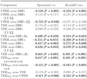
Table 3. Results of statistical analyses comparing diversity with preservational and sampling proxies. See Table 1 for an explanation of the abbreviations of diversity curves and proxies and Table 2 for other abbreviations. Statistically significant results are in bold
Comparison Spearman’s rs Kendall’s tau
UPDE versus DBFs −0.526 (P < 0.001) −0.334 (P = 0.001) UPDE versus DBFs
(LT-EJ)
0.112 (P= 0.717) 0.121 (P= 0.610) UPDE versus DBFs (EJ) −0.733 (P = 0.048) −0.537 (P = 0.100) TDE versus DBFs 0.174 (P= 0.221) 0.114 (P= 0.257) TDE versus DBFs (LT-EJ) 0.290 (P= 0.333) 0.160 (P= 0.498) TDE versus DBFs (K) 0.490 (P= 0.020) 0.314 (P= 0.043) UPDE versus DBCs −0.355 (P = 0.013) −0.260 (P = 0.011) TDE versus DBCs 0.427 (P= 0.002) 0.272 (P= 0.008) TDE versus DBCs (LT-EJ) 0.636 (P= 0.018) 0.470 (P= 0.036) TDE versus DBCs (K) 0.663 (P < 0.001) 0.491 (P < 0.001) TDEWEversus terrestrial rock 0.617 (P < 0.001) 0.501 (P < 0.001) TDEWEversus marine
rock
−0.555 (P < 0.001) −0.445 (P < 0.001) TDEWEversus TDE 0.119 (P= 0.381) 0.095 (P= 0.377)
TDEWEversus UPDE 0.411 (P= 0.006) 0.332 (P = 0.005)
making them broadly comparable. Higher taxic levels (e.g. families) have been demonstrated to be unsuitable proxies for genera in macroevolutionary studies (e.g. Rhodes & Thayer, 1991; Smith, 1994; Barrett & Upchurch, 2005; Tarver, Braddy & Benton, 2007) and were not examined here. Analyses have thus been implemented at the generic level: because it was conducted at the specific level, the supertree of Lloyd et al. (2008) is the exception. In this supertree, a number of species belonging to individual genera were recovered as paraphyletic (e.g. Haplocanthosaurus and Brachiosaurus); therefore each species included in the supertree is considered a unique taxon for the purposes of this study. For phylogenetic diversity curves, the taxa used are restricted to those genera incorporated into the original analyses; however, the taxic diversity curve incorporates all valid sauropodomorph taxa. As a result, the taxic diversity estimate (TDE) incorporates almost twice as many taxa as that of the largest phylogenetic diversity estimate (PDE). This is a consequence partly of the description of numerous taxa since the publication of these phylogenies, but also pertains to the large amount of missing data in taxa represented by very incomplete (or poorly described) specimens that cannot be incorporated into large-scale phylogenetic analyses. However, to attempt to remove any bias, we also compare pruned versions of the TDE with the PDE. This is implemented by restricting the TDE in these comparisons to just those taxa present in the phylogenetic analysis.
(d) Geological age of taxa
One of the most serious issues with constructing diversity curves is that the geological ages of taxa often cannot be
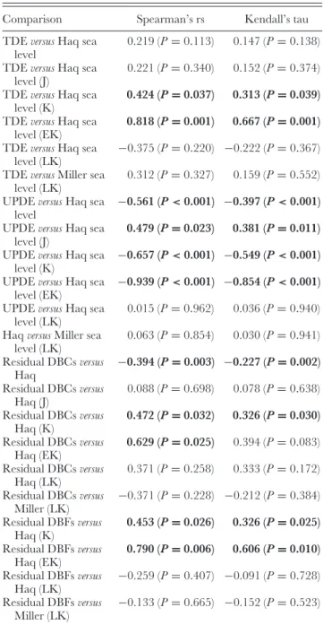
Table 4. Results of statistical analyses comparing observed and ‘corrected’ diversity with sea level. See Table 1 for an explanation of the abbreviations of diversity curves and proxies and Table 2 for other abbreviations. Haq = Haq et al. (1987), Miller = Miller et al. (2005). Statistically significant results are in bold
Comparison Spearman’s rs Kendall’s tau
TDE versus Haq sea level
0.219 (P= 0.113) 0.147 (P= 0.138) TDE versus Haq sea
level (J)
0.221 (P= 0.340) 0.152 (P= 0.374) TDE versus Haq sea
level (K)
0.424 (P= 0.037) 0.313 (P= 0.039) TDE versus Haq sea
level (EK)
0.818 (P= 0.001) 0.667 (P= 0.001) TDE versus Haq sea
level (LK)
−0.375 (P = 0.220) −0.222 (P = 0.367) TDE versus Miller sea
level (LK)
0.312 (P= 0.327) 0.159 (P= 0.552) UPDE versus Haq sea
level
−0.561 (P < 0.001) −0.397 (P < 0.001) UPDE versus Haq sea
level (J)
0.479 (P= 0.023) 0.381 (P= 0.011) UPDE versus Haq sea
level (K)
−0.657 (P < 0.001) −0.549 (P < 0.001) UPDE versus Haq sea
level (EK)
−0.939 (P < 0.001) −0.854 (P < 0.001) UPDE versus Haq sea
level (LK)
0.015 (P= 0.962) 0.036 (P= 0.940) Haq versus Miller sea
level (LK) 0.063 (P= 0.854) 0.030 (P= 0.941) Residual DBCs versus Haq −0.394 (P = 0.003) −0.227 (P = 0.002) Residual DBCs versus Haq (J) 0.088 (P= 0.698) 0.078 (P= 0.638) Residual DBCs versus Haq (K) 0.472 (P= 0.032) 0.326 (P= 0.030) Residual DBCs versus Haq (EK) 0.629 (P= 0.025) 0.394 (P= 0.083) Residual DBCs versus Haq (LK) 0.371 (P= 0.258) 0.333 (P= 0.172) Residual DBCs versus Miller (LK) −0.371 (P = 0.228) −0.212 (P = 0.384) Residual DBFs versus Haq (K) 0.453 (P= 0.026) 0.326 (P= 0.025) Residual DBFs versus Haq (EK) 0.790 (P= 0.006) 0.606 (P= 0.010) Residual DBFs versus Haq (LK) −0.259 (P = 0.407) −0.091 (P = 0.728) Residual DBFs versus Miller (LK) −0.133 (P = 0.665) −0.152 (P = 0.523)
constrained with precision. Few fossil taxa can be directly dated (e.g. by radiometric dating), and even when they can the dates obtained are usually restricted to the horizons above and/or below the fossil-bearing layer. Most vertebrate fossils are dated using indirect methods, such as biostratigraphy, which tend to be limited in resolution to the stage level (e.g. Campanian; 83.5–70.6 Myr), or even coarser time bins, and can impose some circularity depending on the taxa involved. For the Mesozoic, stage intervals vary in temporal range
from approximately 3 to 13 Myr in duration (Gradstein et al., 2005); thus, any fossil indirectly dated will have an associated error in its temporal range. Many sauropodomorph fossils cannot be dated more accurately than to the epoch level (e.g. Middle Jurassic), with an animal dated as Early Cretaceous confined only to a 46 Myr period. For example, estimates for the age of the Chinese somphospondyl Euhelopus (see Fig. 1) span a 39 Myr interval from the Tithonian through to the Aptian (150.8–112.0 Myr; Wilson & Upchurch, 2009).
As long as error is randomly distributed, it can only degrade a genuine signal: it cannot create an artificial one (Raup, 1991; Smith, 2001). Previous workers (e.g. Sepkoski, 1993; Adrain & Westrop, 2000) have demonstrated that stratigraphical and taxonomic revisions have had little significant effect on overall diversity patterns. Thus, although the most recent literature has been used as the basis for our stratigraphic ranges and taxonomy, we do not expect the overall observed diversity curve to differ greatly from those of previous studies. In most instances we use the full suggested temporal span of a taxon, although in some cases we utilise estimates based on more accurate dating techniques. A full list of stratigraphic ranges is included with the list of taxa in the online Appendix.
(3) Preservational biases and sampling quality
Taphonomic and sampling biases have the potential to affect greatly observed generic richness in the fossil record, and thus the accurate reconstruction of diversity curves for fossil taxa (e.g. Behrensmeyer, Kidwell & Gastaldo, 2000; Miller, 2000; Alroy et al., 2001, 2008; Upchurch & Barrett, 2005; Smith, 2007; Smith & McGowan, 2007; Uhen & Pyenson, 2007; Peters, 2008; Barrett et al., 2009; Butler et al., 2009c; Wall, Ivany & Wilkinson, 2009; Benson et al., 2010). Following the work of Raup (1972), numerous investigators have demonstrated that both the amount of rock outcrop and the environments preserved therein have varied throughout geological time (e.g. Ronov et al., 1980; Schindel, 1980; Sadler, 1981; Kalmar & Currie, 2010). For example, the ratio of terrestrial to marine environments at any time interval is dependent upon sea level (Smith & McGowan, 2007). As a consequence of this, diversity might simply mirror the amount of rock outcrop and the number of opportunities to observe fossils (NOOs: Raup, 1972, 1976; Alroy et al., 2001; Peters & Foote, 2001, 2002; Smith, 2001; Smith, Gale & Monks, 2001; Crampton et al., 2003; Peters, 2005, 2008; Smith & McGowan, 2005, 2007; Upchurch & Barrett, 2005; Uhen & Pyenson, 2007; Fr¨obisch, 2008; McGowan & Smith, 2008; Barrett et al., 2009; Butler et al., 2009c; Marx, 2009; Benson et al., 2010). Thus, apparent diversity cannot be entirely controlled by rock outcrop or the NOOs if it is to reflect genuine evolutionary patterns. Therefore, we consider a range of sampling proxies in our comparisons with sauropodomorph diversity, in an attempt to tease apart any genuine biological signal from that of the rock record.
(a) Rock outcrop
Upchurch & Barrett (2005) and Barrett et al. (2009) utilised dinosaur-bearing formations (DBFs) as a proxy for rock outcrop (based on data from Weishampel et al., 2004a), plotting the number of DBFs through time. These authors chose to use DBFs rather than sauropodomorph-bearing formations (as utilised by Hunt et al., 1994) because if a rock unit is capable of preserving large terrestrial vertebrates (i.e. any dinosaur) then it should also be capable of preserving sauropodomorphs; i.e. rock units lacking (or with low diversities of ) sauropodomorphs, but preserving other dinosaurs, may reflect genuine situations where sauropodomorph diversity was depauperate. Thus, here we also use DBFs for our updated diversity analyses.
A more refined version of using DBFs is to quantify the rock record itself. Peters & Foote (2001) estimated the amount of marine sedimentary rock outcrop at epoch level for the Phanerozoic of the USA and noted that fluctuations are positively correlated with generic marine diversity. Wall et al. (2009) also recovered a strong correlation between epoch-level Phanerozoic marine diversity and global rock outcrop, albeit through implementing a much coarser global estimate. A global correlation was also noted between the amount of terrestrial sediment (at epoch level) and continental fossil richness (Kalmar & Currie, 2010). Similarly, Smith & McGowan (2007) calculated outcrop area of marine and terrestrial sediments at stage level for the Phanerozoic of western Europe. They found that the size and timing of two of the five major Phanerozoic mass extinctions are strongly predicted by rock outcrop but concluded that overall diversity trends (as well as the K/P extinction event) were not the result of rock area bias. For the purposes of this study, we utilise the terrestrial and marine rock record data of Smith & McGowan (2007) to construct Mesozoic rock outcrop curves. We then compare this with the diversity curves produced for Sauropodomorpha (TDE and PDE), as well as taxic diversity from western Europe alone (TDEWE) in an attempt to clarify whether this region provides a suitable proxy for the global rock record (at least for sauropodomorphs).
(b) Collecting effort
As well as geological biases (see above), additional human biases exist in terms of taxonomic artefacts (Uhen & Pyenson, 2007; Alroy et al., 2008; Peters, 2008) and the disproportionate sampling and study of different time intervals (e.g. the Campanian–Maastrichtian has received considerably more attention than most other Mesozoic stages). McGowan & Smith (2008) also highlighted the likelihood of the global Phanerozoic diversity curve being disproportionately influenced by European and North American fossil data.
Collection-based methods have been used by previous authors in attempts to investigate the diversity of numerous groups (e.g. Crampton et al., 2003; Uhen & Pyenson, 2007; Alroy et al., 2008; Carrano, 2008a). Thus, in addition to utilising DBFs and rock outcrop, we
compare diversity with the number of dinosaur-bearing collections (DBCs) per unit time, derived from the Paleobiology Database (www.pbdb.org; Carrano, 2008b). These collections represent discrete, independent samples of dinosaurs from specific geographic and stratigraphic localities; they have been as finely resolved as the published record allows.
An additional way to assess collecting effort is to construct collector curves for fossil taxa by plotting the cumulative number of newly described taxa against the date of description. When the rate of new discoveries declines markedly, it is assumed that true diversity (at least in terms of those taxa that were fossilised and thus had a chance of being discovered) has been approached (Benton, 1998). The near-complete collector curve should thus have a sigmoid shape with a slow initial rise followed by a phase of rapid increase, before levelling off towards an asymptote (Benton, 1998, 2008). Another method is to look for correlations between the geological ages of taxa and their years of description. If we were increasingly driving back (or forward) the age of the oldest (or youngest) taxon, then we might suspect that there were large gaps in our sampling (Benton, 1998; Fountaine
et al., 2005). If, at the other end of the spectrum, the fossil
record was extremely well sampled then we might expect new discoveries to be from geological ages from which we already have numerous taxa. A more likely scenario is that new discoveries from an overall well-sampled fossil record will fill in the various internal stratigraphic gaps within that record. Here we utilise both of these measures to assess further the contribution of human error in estimating diversity. (c) Residuals
The effect of sampling biases on diversity can also be analysed by constructing a model in which sampling opportunity perfectly predicts the TDE, then subtracting this from the TDE, leaving a residual ‘unexplained diversity signal’ (Smith & McGowan, 2007; Barrett et al., 2009; Butler et al., 2009c; Benson et al., 2010). These models have been constructed by independently sorting log sampling bias (e.g. DBFs and DBCs) and log TDE from low to high values, then fitting a linear model of the form y= mx + c to the ordered data, where x is the sampling proxy datum, m is the gradient of the line and c is a constant.
We apply this equation to the sampling bias data in its original order (i.e. plotted against geological time) to derive a temporal series of modelled (or predicted) diversity (MDE). Lastly, we subtract MDE from TDE to obtain the residual, which therefore represents fluctuations in diversity that cannot be explained in terms of the sampling bias (Smith & McGowan, 2007; Barrett et al., 2009; Butler et al., 2009c; Benson et al., 2010). We then repeat this last step, replacing TDE with PDE (Barrett et al., 2009), to obtain residuals of PDE from MDE. Using this residuals-based method, we then compare TDE and PDE with the sampling biases outlined in the preceding sections. Time periods in which residuals vary between different sampling biases could help in identifying which factors affect particular temporal intervals.
(d) Rarefaction
One of the fundamental problems with diversity analyses is their dependence on sample size (Sanders, 1968; Raup, 1975; Colwell & Coddington, 1994). To overcome this problem, Sanders (1968) developed the method of rarefaction (later built upon and discussed further by: Hurlbert, 1971; Simberloff, 1972; Heck, Van Belle & Simberloff, 1975; Raup, 1975; Tipper, 1979; Gotelli & Colwell, 2001; Hammer & Harper, 2006) to compare taxonomic richness in samples of different sizes and to investigate the effect that sample size has upon taxon counts (Hammer & Harper, 2006).
Rarefaction has been used to address a wide range of problems in palaeobiology, including: the effects of sample size on diversity (e.g. Miller & Foote, 1996), estimates of taxonomic richness (e.g. Fastovsky et al., 2004) and abundance (e.g. Davis & Pyenson, 2007); morphological variety (Foote, 1992); comparisons of diversity between biofacies and sea-level changes (e.g. Westrop & Adrain, 1998); and fluctuations in diversity at extinction and radiation events (e.g. Adrain et al., 2000).
Nearly all analyses of dinosaur diversity have been limited to counts of numbers of taxa or lineages per stage. Thus far, only one published study (Fastovsky et al., 2004) has implemented rarefaction in an attempt to elucidate global dinosaur diversity [although studies by Sheehan et al., (1991) and Pearson et al., (2002) have also used rarefaction to address regional diversity]: Fastovsky et al. (2004) utilised the global dinosaur locality dataset of Weishampel et al. (2004a), pruning it to exclude generically indeterminate material. These authors demonstrated a steady increase in diversity throughout the Mesozoic and argued that dinosaurs were not in decline in the last 10 Myr of the Mesozoic (see also Sheehan et al., 1991; Pearson et al., 2002; Wang & Dodson, 2006). This study has been criticised by several workers (Archibald, 2005; MacLeod & Archibald, 2005; Sullivan, 2006), who questioned the interpretation of the rarefied data by Fastovsky et al. (2004) and suggested (after re-analysis) that a Maastrichtian decline in dinosaur diversity is still well supported. However, Carrano (2008a) demonstrated that dinosaur diversity for the latest Cretaceous of North America shows much less variation among formations and time intervals than is documented by stage-level diversity counts and suggested that, rather than reflecting an end-Cretaceous decline, Campanian–Maastrichtian fluctuations (at least for North America) are the product of ecological, environmental and sampling biases (particularly of an anthropogenic nature).
Following Fastovsky et al. (2004), we omit all generically indeterminate occurrences from our global database. We then split generic occurrences into their respective stratigraphic stages, and count each taxon as present for each interval in which it occurred (see online Appendix). Smaller time bins (i.e. substage) are not used because of constraints on minimum sample sizes for effective rarefaction (Krebs, 1999; Hammer & Harper, 2006). Sample-based rarefaction (using the number of localities each genus is found at in each stage) is implemented in PAST (Hammer et al., 2001),
with only time bins (7) containing 30+ samples rarefied, and curves of rarefied diversity are constructed.
One potential problem with this method of rarefaction is the omission of generically indeterminate occurrences. Previous rarefaction analyses have excluded these and have only included numbers of occurrences of genera. However, in a given sample, it is unlikely that all individuals will be recognised to the level of genus: many sauropodomorph individuals cannot be recognised beyond clade or family level (e.g. Titanosauria). As such, a modified version of the rarefaction analysis is also implemented. For each locality, an additional genus is included for material representing any clade that cannot include any of the named genera. For example, if a site contains remains of Dicraeosaurus, as well as indeterminate diplodocid and diplodocoid elements, then its total generic diversity would be two because the indeterminate diplodocid materials cannot be referred to
Dicraeosaurus (a dicraeosaurid diplodocoid; see Fig. 1) and
must belong to a second taxon. However, the indeterminate diplodocoid could represent undiagnostic materials of either form and is thus not counted. The same procedure is applied when only indeterminate materials are present (i.e. two genera are considered present in a quarry that preserves indeterminate dicraeosaurid, diplodocid and diplodocoid materials). These indeterminate occurrences are summed and considered additional genera for each time bin. As well as enabling the inclusion of indeterminate materials and thereby attempting to assess ‘cryptic’ diversity, our method also has the advantage of greatly increasing the sample size for each time bin, which has obvious benefits for rarefaction (i.e. increasing the size of the smallest sample). Sample-based rarefaction, using ‘all occurrences’, is implemented at several different minimum sample sizes: 30 (22 stages included), 50 (18 stages), 70 (11 stages) and 90 (7 stages). Lastly, to test previous suggestions of a latest-Cretaceous diversity decline, we implement substage-level ‘all occurrences’ rarefaction for the Campanian-Maastrichtian, using the early (sample size= 64) and late (sample size = 83) Campanian as our smallest sample sizes.
One issue concerns the choice of time bins, as stages vary in duration. Rarefaction is time dependent, so we would expect to sample more taxa during longer time periods; thus, it is perhaps best to use time bins of approximately equal duration (Raup, 1975; Alroy et al., 2001, 2008). We might expect that more genera were present during longer time intervals than short ones, even when both had similar levels of diversity at any one point in time. Additionally, there may be a higher chance of genera being preserved given a longer time period. For example, the Early Cretaceous is 45.9 Myr while the Late Jurassic is only 15.7 Myr in duration. Similarly, the Campanian represents a time interval of 12.9 Myr while the Hettangian is only 3.1 Myr in duration. However, when TDE and length of stage and epoch are compared, we find no statistically significant correlations (P > 0.3 for all tests). In addition, there is no correlation between time bin duration and number of samples (P > 0.1 for all tests). Consequently, our choice of time bins seems adequate for these analyses.
(4) Comparisons with sea level
Closely related to the rock record is the record of fluctuating sea levels (Haq, Hardenbol & Vail, 1987). It has long been noted that eustatic Phanerozoic sea-level fluctuations coincide with many episodes of variation in marine diversity (Newell, 1952; Johnson, 1974; Hallam, 1989; Smith, 2001). Other workers have also observed a close correlation between patterns of sauropodomorph (and/or dinosaur) diversity and sea-level fluctuations (Haubold, 1990; Hunt et al., 1994; Upchurch & Barrett, 2005). Although sauropodomorphs were terrestrial, sea level could have affected their apparent diversity abiotically, e.g. through controlling their preservation potential (Upchurch & Barrett, 2005). The remains of terrestrial organisms may be more likely to reach aquatic environments during periods of high sea level, meaning they are more likely to be preserved (Haubold, 1990). Additionally, coastal and marginal marine environments potentially stand a better chance of being preserved during transgressive phases (A. B. Smith, personal communication 2009). If correct, high sea level should be correlated with high observed diversity (assuming that genuine diversity fluctuations do not obscure the effects of variations in preservation rates). The opposite effect has also been proposed: the available land area on which to preserve a terrestrial record could be greatly reduced during times of high sea level, resulting in a poorer fossil record (Markwick, 1998). Other workers have proposed biotic factors that might cause sea level to be positively or negatively correlated with genuine diversity. For example, in terrestrial animals, allopatric speciation is likely to happen during high sea levels as land areas become separated, whereas during low sea levels there may be mixing of previously isolated organisms, potentially resulting in extinctions (Bakker, 1977; Horner, 1983; Weishampel & Horner, 1987). Conversely, the formation of geographic barriers may also result in extinction events as the sizes of some habitats dwindle (Dodson, 1990; Upchurch & Barrett, 2005).
The current study replicates earlier analyses by comparing both observed (TDE) and ‘corrected’ sauropodomorph diversity (i.e. PDE, residuals and rarefaction) with the sea-level curve of Haq et al. (1987). By using both observed and ‘corrected’ diversity, we can attempt to tease apart biotic and abiotic effects of sea level on diversity. In addition, we implement a finer scale study to look for correlations solely during the Late Cretaceous, utilising a recently developed backstripped sea-level curve (Miller et al., 2005), which represents the global sea-level record for the past 100 Myr. For both sea-level curves, average sea level is calculated for each substage time bin. It should be noted, however, that the stratigraphy of Haq et al. (1987) differs considerably from the recent Gradstein et al. (2005) timescale. For example, the Oxfordian is dated as 145–152 Ma in the former and 155.7–161.2 Ma in the latter, while the Jurassic/Cretaceous boundary is dated at 131 Ma in the Haq et al. (1987) study but is now dated at 145.5 Ma (Gradstein et al. 2005). Thus, the re-calibrated Mesozoic sea-level data of Haq et al. (1987) [as listed in Miller et al. (2005)] are used here.
(5) ‘Summary’ diversity
Lastly, we present a ‘summary’ diversity curve; this is constructed qualitatively and diversity fluctuations are relative. Peaks and troughs common to all three estimates (PDE, residuals and rarefaction) are considered genuine, and correspondingly when all three indicate the effect of sampling biases then observed diversity is considered an artefact. When our diversity estimates contradict one another, we take an ‘average’, e.g. if two estimates show peaks but one demonstrates the effect of sampling, then we consider this a small diversity peak. Where this contradiction is more significant (i.e. some estimates show a peak and some show a trough), we illustrate both possible diversity curves.
III. ANALYSES AND RESULTS
In this section we outline and present the results of the various analyses implemented, beginning with a description of the updated TDE. The comparisons between the different PDEs are also reported, as are our statistical tests between diversity (both TDE and PDE) and sampling proxies. Lastly, we present the statistical comparisons between our diversity curves and sea level.
(1) Sauropodomorph taxic diversity
The updated taxic diversity curve (Fig. 5) largely follows previous analyses (Fig. 4; Barrett & Upchurch, 2005; Upchurch & Barrett, 2005; Barrett et al., 2009); only two slight differences will be commented on. Firstly, a diversity trough in the Oxfordian was demonstrated by both Upchurch & Barrett (2005) and Barrett et al. (2009), and the new TDE agrees with this, but indicates that this represents the nadir in sauropodomorph diversity. Secondly, the TDE shows an early Maastrichtian increase in diversity from the Campanian, with the magnitude of this peak close to that of the Kimmeridgian–Tithonian apex. Such a substantial peak has not been reported in previous sauropodomorph diversity analyses [although notable peaks are apparent in Upchurch & Barrett (2005) and Barrett et al. (2009)] and reflects the large number of taxa named from the latest Cretaceous in recent years (e.g. Maxakalisaurus and Uberabatitan), subsequent to the publication of these earlier diversity analyses.
(2) Statistical comparisons between phylogenetic and taxic diversity
A diversity curve based on a composite cladogram of Upchurch et al. (2004, 2007) (UPDE) was compared with curves derived from the basal sauropodomorph and sauropod diversity curves of Yates (2007) (YPDE) and Wilson (2002) (WPDE), respectively. Comparisons were also made between UPDE and taxic diversity (TDE), as well as the sauropodomorph element of the supertree of Lloyd et al. (2008) (LPDE), in an attempt to elucidate sauropodomorph diversity. UPDE and TDE were also compared with the
Fig. 5. Updated sauropodomorph taxic diversity estimate (TDE) through the Mesozoic. See Fig. 3 for abbreviations.
diversity curves of Barrett et al. (2009) (BTDE and BPDE). To make statistical comparisons more meaningful, only the basal sauropodomorph element of the UPDE (i.e. Upchurch
et al., 2007) was compared with YPDE; similarly, only the
sauropod element of the UPDE (i.e. Upchurch et al., 2004) was compared with WPDE. Lastly, the pruned versions of TDE (i.e. the TDE reduced to just those taxa present in the phylogenetic diversity estimates: TDEP) were compared with the UPDE and LPDE (i.e. the phylogenies which sample all sauropodomorphs). Fig. 6 displays the UPDE, LPDE, YPDE and WPDE curves, while Table 2 reports the statistical comparisons.
Overall, UPDE and YPDE are strongly correlated with one another, whereas UPDE and WPDE display a moderately strong correlation (see Table 2). The correlation between UPDE and TDE is considerably weaker, although when restricted to just the Late Triassic–Jurassic, this
correlation is extremely strong (while there is no correlation between the two curves for the Cretaceous; Table 2). UPDE and TDE are strongly correlated with BPDE and BTDE, respectively, but show no, or only a very weak, correlation when the phylogenetic and taxic diversity estimates are compared (Table 2). UPDE and TDE show only a weak correlation with LPDE and this disappears when the Cretaceous is examined separately. LPDE does not show
any closer correlation when compared to TDEP; however,
UPDE is correlated with TDEP even for the Cretaceous
(Table 2; cf. UPDE versus TDE for the Cretaceous).
(3) Statistical comparisons between diversity and sampling proxies
UPDE and TDE have been compared with numbers of DBFs and DBCs, as well as western European rock outcrop area (Figs. 7–8). Overall, there is a negative correlation between
Fig. 6. Sauropodomorph phylogenetic diversity estimates (PDEs) through the Mesozoic. Black solid line= UPDE; grey solid line =
YPDE; grey dashed line= WPDE; black dotted line = LPDE. See Table 1 for explanation of the abbreviations for the diversity curves and Fig. 3 for abbreviations of geological stages.
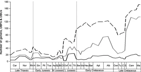
Fig. 7. Taxic diversity estimate (TDE) plotted against numbers of dinosaur-bearing formations (DBFs) and dinosaur-bearing
collections (DBCs). Black solid line= TDE; black dashed line = DBFs; grey solid line = DBCs. Note that DBCs have been divided by 10 to allow the curves to be plotted together. See Fig. 3 for abbreviations.
DBFs and the UPDE, but no significant correlation with the TDE (see Table 3). Barrett et al. (2009) also found only a weak correlation between sauropodomorph genus richness and DBFs and commented (p. 2671) that ‘the latter measure is an exceptionally poor predictor of sauropodomorph diversity’. There is no correlation between the UPDE and DBFs when we consider smaller time bins (period and epoch), with the exception of a moderately strong, negative correlation in the Early Jurassic (Table 3). The number of DBCs is positively correlated with the TDE for the Mesozoic and has a weakly negative correlation with the UPDE (Table 3).
A correlation exists between DBCs and TDE for the Late Triassic–Early Jurassic, while the TDE (but not the UPDE) shows a significant correlation with both DBFs and DBCs when only the Cretaceous is considered (Table 3).
There is no correlation between either the TDE or UPDE and terrestrial western European rock outcrop area. Furthermore, there is no correlation when diversity and marine rock outcrop are compared (Table 3). However,
when only western European taxic diversity (TDEWE) is
considered, there is a relatively strong correlation with both terrestrial (positive) and marine (negative) rock area (see
Fig. 8. Taxic diversity estimate (TDE) plotted against terrestrial and marine rock outcrop area (based on numbers of maps with
outcrop; Smith & McGowan, 2007). Black solid line= TDE; grey solid line = terrestrial rock; black dotted line = marine rock. Note that the rock outcrop values have been divided by 10 to allow the curves to be plotted together. See Fig. 3 for abbreviations.
Fig. 9. Residual diversity through time: (A) Taxic diversity estimate (TDE)-based residuals using dinosaur-bearing collections (DBCs)
for the Mesozoic; (B) Upchurch et al. (2004, 2007) phylogenetic diversity estimate (UPDE)-based residuals using dinosaur-bearing formations (DBFs) for the Early Jurassic; (C) TDE-based residuals using DBFs for the Cretaceous. See Fig. 3 for abbreviations.
Table 3). TDEWE shows no correlation with global TDE
but, slightly surprisingly, is correlated with the UPDE.
(4) Residuals and rarefaction
As noted in Section II. 3c, residuals were implemented only for those proxies correlated with diversity, and only for the particular time intervals where the correlation
occurs. TDE-based residuals were thus constructed for DBCs throughout the Mesozoic, as well as for Cretaceous DBFs (Fig. 9). UPDE-based residuals were constructed only for Early Jurassic DBFs. The residual peaks and troughs are described in Section IV.
Implementation of ‘genus-only’ rarefaction allows only a few observations to be made regarding fluctuations in diversity, because of sizable error bars (Fig. 10). Similar
Fig. 10. Rarefied diversity through time: (A) genus-only occurrences (sample size= 30); (B) all-occurrences (sample size = 30);
(C) all-occurrences (sample size= 70); (D) all-occurrences (sample size = 90). 95% confidence error bars are plotted on each diversity curve. See Fig. 3 for abbreviations.
problems affect the ‘all-occurrences’ rarefaction; however, much more is discernible from these diversity plots (Fig. 10). Those peaks and troughs that can be distinguished are commented upon in Section IV. No fluctuations in diversity could be determined from our substage-level rarefaction for the latest Cretaceous.
(5) Historical collecting effort
In total, 175 sauropodomorph taxa are considered valid herein (see online Appendix). Their cumulative rate of discovery displays no asymptote and is in the rapid increase phase (see Fig. 4 in Mannion & Upchurch, 2010b), suggesting that many more genera remain to be discovered (Benton, 1998; Wang & Dodson, 2006). New discoveries are not driving back the geological age of the oldest sauropodomorphs [e.g. Thecodontosaurus, from the late Carnian–Rhaetian of the UK, was the first sauropodomorph to be scientifically described (Riley & Stutchbury, 1836) and still remains one of the oldest known], nor are they extending our knowledge into younger time periods [e.g. Magyarosaurus from the late Maastrichtian of Romania was described by Nopcsa (1915), but no Paleogene sauropods have been recovered subsequently]. However, new discoveries are filling many gaps in the sauropod fossil record, e.g. Bonitasaura and
Futalognkosaurus have been named in recent years from the
early Late Cretaceous, an interval which previously yielded very little sauropod material.
Of these 175 valid taxa, 50 come from Asia and 46 from South America. 30 taxa have been described from Europe, 25 from Africa, and 21 from North America; just two have been described from Australasia and only one from Antarctica. Three countries account for over half of
all sauropodomorph diversity: Argentina (38 taxa), China (36 taxa) and the USA (20 taxa). Over half (101 genera) of sauropodomorph taxa are from Laurasia, with 74 from the approximately equally sized Gondwana (Smith, Smith & Funnell, 1994). Given their similarity in surface area, this distributional skew almost certainly reflects the Northern Hemisphere origin of dinosaur palaeontology: for example, note that just two Gondwanan taxa were named prior to the 1910s, compared to 20 Laurasian taxa.
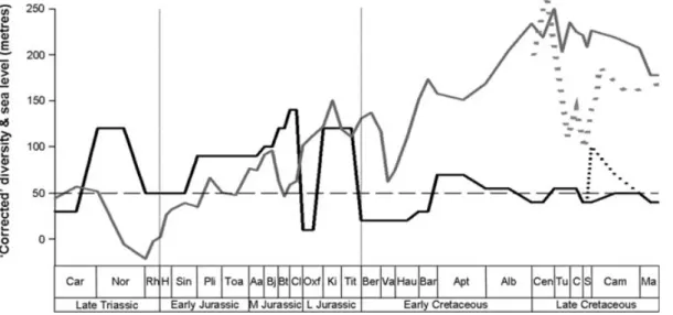
(6) Comparisons between sea level and diversity
The sea level curve of Haq et al. (1987; Fig. 11) was statistically compared with observed (TDE) and ‘corrected’ diversity; it was also qualitatively compared with ‘summary’ diversity (see Section IV). Comparisons were also made with the Late Cretaceous element of the Miller et al. (2005) curve. There is no correlation between the TDE and sea level for the Mesozoic; however, a strong positive correlation is recovered when the Cretaceous and Early Cretaceous are examined separately (Table 4). All other time-slices produce non-significant results.
Sea level is positively correlated with the UPDE for the Jurassic and strongly negatively correlated when the Early Cretaceous is examined. However, there is no correlation between diversity and sea level when comparisons are limited to the Late Triassic–Early Jurassic or Late Cretaceous time intervals.
There is only a weak negative correlation between DBC-based residuals and sea level for the Mesozoic (Table 4). There is no correlation when we compare the two for the Jurassic or Late Cretaceous separately, but there is a statistically significant positive correlation between
Fig. 11. ‘Summary’ diversity plotted against sea level (Haq et al., 1987; Miller et al. 2005). Black solid line= ‘summary’ diversity;
black dotted line= alternative Campanian–Maastrichtian ‘summary’ diversity; grey solid line = Haq et al. (1987) sea level; grey dotted line= Miller et al. (2005) sea level; black dashed (horizontal) line = sampling biases. Note that the y-axis values are for sea level only; ‘summary’ diversity only shows relative fluctuations in diversity (see text for explanation of construction). Note that the Miller et al. (2005) sea level values have been multiplied by 3 to allow the two sea level curves to be plotted together. See Fig. 3 for abbreviations.
DBC-based residuals and sea level in the Early Cretaceous (Table 4). A moderately strong positive correlation between DBF-based residuals and sea level is recorded for the Cretaceous (Table 4). This correlation disappears when we examine the Late Cretaceous by itself, but is greatly reinforced when only the Early Cretaceous is considered (Table 4).
As a consequence of the rarefied datasets excluding various stages because of sample sizes, a meaningful statistical comparison with sea level cannot be implemented. However, comparison of the individual peaks and troughs are included in Section IV.
IV. DISCUSSION
(1) ‘Summary’ diversity through time
(a) Late Triassic
The UPDE and YPDE both show an initial increase in diversity from the Carnian (228.0–216.5 Myr) to a peak in the Norian (216.5–203.6 Myr), before a steep decline in the Rhaetian (203.6–199.6 Myr; Fig. 6). This pattern was also noted by Barrett & Upchurch (2005) and Barrett et al. (2009). However, consideration of residuals suggests that genus richness was low in the Carnian, whereas diversity in the Rhaetian appears to be partly controlled by sampling biases. These results contrast with previous suggestions that the late Norian/Rhaetian (203.6 Myr) represents one of the major Phanerozoic extinction events (see Bambach, 2006, and references therein; Arens & West, 2008), although this extinction has mostly been associated with marine faunas [Benton, 1994; but see Benson et al. (2010) for a conflicting result regarding marine reptiles]. Diversity in the Norian does appear to be genuinely high (Figs 9–11), reflecting the diversification of ‘prosauropods’ and basal sauropodomorphs.
(b) Early Jurassic
The UPDE shows a slight increase in diversity from the Rhaetian (but less than the Norian peak), whereas the YPDE shows a continued decline (Fig. 6). The WPDE and BPDE also show a Hettangian (199.6–196.5 Myr) increase in genus richness. Following this increase, the UPDE curve remains relatively flat, whereas the YPDE continues to decline until a diversity increase in the Pliensbachian (189.6–183.0 Myr; Fig. 6). Barrett et al. (2009) demonstrated a similar diversity plateau as in the UPDE but differed in showing a notable Toarcian (183.0–175.6 Myr) decline. Residuals and rarefaction indicate that diversity in the Hettangian–Sinemurian is controlled by sampling, whereas the Pliensbachian–Toarcian peak appears genuine (Figs 9–11), perhaps reflecting the onset of eusauropod diversification. There is no evidence for a late Pliensbachian–early Toarcian extinction event, in contrast
to that among marine taxa (Harries & Little, 1999; Bambach, 2006; Arens & West, 2008).
(c) Middle Jurassic
Although the YPDE and WPDE both show a steep drop in diversity in the Aalenian (175.6–171.6 Myr) (by which point non-eusauropod sauropodomorphs were replaced by eusauropods: Barrett & Upchurch, 2005), UPDE shows diversity levels comparable to the Toarcian (Fig. 6). Although the extinction of basal forms explains why the YPDE drops at this point, this factor cannot explain the differences between the other two curves; this peak in the UPDE can be explained by the inclusion of Bellusaurus, which is discussed in Section IV. 2. Following this, the UPDE and WPDE both show an increase in diversity, and all measures indicate a peak in the Bathonian–Callovian (167.7–161.2 Myr; Figs 6, 11), reflecting the neosauropod radiation (although residuals indicate a diversity peak throughout the Middle Jurassic; Figs 9, 10).
(d) Late Jurassic
All measures recover a severe decline in diversity in the Oxfordian (161.2–155.7 Myr; Upchurch & Barrett, 2005; Barrett et al., 2009), followed by a peak in the Kimmeridgian–Tithonian (155.7–145.5 Myr). Thus, it appears that the Oxfordian was a genuine time of depauperate diversity (Upchurch & Barrett, 2005) (although see Section IV. 4), whereas the Kimmeridgian–Tithonian diversity peak seems to represent a real biological event (Figs. 9–11), and is not an artefact of sampling.
(e) Early Cretaceous
All measures show a large drop in diversity at the J/K boundary (145.5 Myr), with taxon richness remaining low at least until the Barremian (130.0–125.0 Myr; Fig. 6). Wagner (2000a) has argued that PDEs should be conservative in detecting mass extinctions, as a consequence of the backward smearing of origination times which diminish the scale of the mass extinction (note that this can only occur if some lineages survive: if the whole group goes extinct, then there are no lineages left to ‘backsmear’). This would suggest that the J/K event potentially represents a genuine extinction (Upchurch & Barrett, 2005; Barrett
et al., 2009). However, the UPDE and WPDE show a
relatively high percentage of ghost lineages in the earliest Cretaceous [in particular the Berriasian (145.5–140.2 Myr): five ghost lineages compared to two actual fossil occurrences (UPDE)]. The increased ‘gappiness’ in the fossil record immediately after mass extinctions has been shown to reflect taphonomic bias (Twitchett, Wignall & Benton, 2000), as Lazarus taxa that temporarily disappear tend to be found in environments that also temporarily disappear (Smith et al., 2001). Thus, this Berriasian ‘gappiness’ may result from lack of preservation of the environments, rather than fluctuations in taxon abundances (Smith, 2001). However, support for a