HAL Id: tel-03208517
https://tel.archives-ouvertes.fr/tel-03208517
Submitted on 26 Apr 2021HAL is a multi-disciplinary open access
archive for the deposit and dissemination of sci-entific research documents, whether they are pub-lished or not. The documents may come from teaching and research institutions in France or abroad, or from public or private research centers.
L’archive ouverte pluridisciplinaire HAL, est destinée au dépôt et à la diffusion de documents scientifiques de niveau recherche, publiés ou non, émanant des établissements d’enseignement et de recherche français ou étrangers, des laboratoires publics ou privés.
Efficiency and Redundancy in Deep Learning Models :
Theoretical Considerations and Practical Applications
Pierre Stock
To cite this version:
Pierre Stock. Efficiency and Redundancy in Deep Learning Models : Theoretical Considerations and Practical Applications. Artificial Intelligence [cs.AI]. Université de Lyon, 2021. English. �NNT : 2021LYSEN008�. �tel-03208517�
Numéro National de Thèse : 2021LYSEN008
THÈSE de DOCTORAT DE L’UNIVERSITÉ DE LYON
opérée parl’École Normale Supérieure de Lyon École DoctoraleN° 512
École Doctorale en Informatique et Mathématiques de Lyon Discipline : Informatique
Soutenue publiquement le 09/04/2021, par :
Pierre STOCK
Efficiency and Redundancy in Deep Learning
Models: Theoretical Considerations and
Practical Applications
Efficience et redondance dans les modèles d’apprentissage
profond : considérations théoriques et applications pratiques
Devant le jury composé de :
Raquel URTASUN, Uber ATG Chief Scientist, Université de Toronto Rapporteure François MALGOUYRES, Professeur des Universités, Université Paul Sabatier Rapporteur Julie DELON, Professeure des Universités, Université Paris Descartes Examinatrice Gabriel PEYRÉ, Directeur de Recherche, CNRS/DMA/ENS ULM Examinateur
Aline ROUMY, Directrice de Recherche, INRIA Examinatrice
Patrick PÉREZ, Scientific Director of Valeo AI Examinateur Rémi GRIBONVAL, Directeur de Recherche, INRIA/ENS de Lyon Directeur de thèse Hervé JÉGOU, Research Director, Facebook AI Research Co-directeur de thèse
Abstract
Deep Neural Networks led to major breakthroughs in artificial intelligence. This unreasonable effectiveness is explained in part by a scaling-up in terms of comput-ing power, available datasets and model size – the latter was achieved by buildcomput-ing deeper and deeper networks. In this thesis, recognizing that such models are hard to comprehend and to train, we study the set of neural networks under the prism of their functional equivalence classes in order to group networks by orbits and to only manipulate one carefully selected representant. Based on these theoretical con-siderations, we propose a variant of the stochastic gradient descent (SGD) algorithm which amounts to inserting, between the SGD iterations, additional steps allowing us to select the representant of the current equivalence class that minimizes a certain energy. The redundancy of the network’s parameters highlighted in the first part nat-urally leads to the question of the efficiency of such networks, hence to the question of their compression. We develop a novel method, iPQ, relying on vector quantization that drastically reduces the size of a network while preserving its accuracy. When combining iPQ with a new pre-conditioning technique called Quant-Noise that injects quantization noise in the network before its compression, we obtain state-of-the-art tradeoffs in terms of size/accuracy. Finally, willing to confront such algorithms to product constraints, we propose an application allowing anyone to make an ultra-low bandwidth video call that is deployed on-device and runs in real time.
R´
esum´
e
Les r´eseaux de neurones profonds sont `a l’origine de perc´ees majeures en intelligence artificielle. Ce succ`es s’explique en partie par un passage `a l’´echelle en termes de puissance de calcul, d’ensembles de donn´ees d’entrainement et de taille des mod`eles consid´er´es – le dernier point ayant ´et´e rendu possible en construisant des r´eseaux de plus en plus profonds. Dans cette th`ese, partant du constat que de tels mod`eles sont difficiles `a appr´ehender et `a entrainer, nous ´etudions l’ensemble des r´eseaux de neurones `a travers leurs classes d’´equivalence fonctionnelles, ce qui permet de les grouper par orbites et de ne manipuler qu’un repr´esentant bien choisi. Ces con-sid´erations th´eoriques nous ont permis de proposer une variante de l’algorithme de descente de gradient stochastique qui consiste `a ins´erer, au cours des it´erations, des ´
etapes permettant de choisir le repr´esentant de la classe d’´equivalence courante min-imisant une certaine ´energie. La redondance des param`etres de r´eseaux profonds de neurones mise en lumi`ere dans ce premier volet am`ene naturellement `a la question de l’efficience de tels r´eseaux, et donc de leur compression. Nous d´eveloppons une nouvelle m´ethode de compression, appel´ee iPQ et reposant sur de la quantification vectorielle, prouvant qu’il est possible de r´eduire consid´erablement la taille d’un r´eseau tout en pr´eservant sa capacit´e de pr´ediction. En combinant iPQ avec une proc´edure de pr´e-conditionnement appel´ee Quant-Noise qui consiste `a injecter du bruit de quan-tification dans le r´eseau avant sa compression, nous obtenons des r´esultats ´etat de l’art en termes de compromis taille/capacit´e de pr´ediction. Voulant confronter nos recherches `a des contraintes de type produit, nous proposons enfin une application de ces algorithmes permettant un appel vid´eo `a tr`es faible bande passante, d´eploy´ee sur un t´el´ephone portable et fonctionnant en temps r´eel.
Remerciements
Je tiens tout d’abord `a remercier les deux rapporteurs, Raquel Urtasun et Francois Malgouyres, pour avoir pris le temps de relire ce manuscrit, pour leurs retours et leurs conseils. Merci ´egalement `a l’ensemble des membres du jury pour leur lecture en profondeur du manuscrit et leurs questions. C’est un honneur de pouvoir soutenir ma th`ese devant un panel de chercheurs aussi accomplis et renomm´es.
Merci `a Herv´e de m’avoir donn´e la chance de m’exprimer `a travers le stage puis la th`ese. La confiance imm´ediate et l’autonomie grisante que tu m’as accord´es m’ont construit en tant que chercheur et m’ont ind´eniablement fait grandir. Un grand merci pour ton accompagnement et ton soutien d´ecisif dans tous les moments cl´es de cette th`ese, aussi bien au niveau scientifique, relationnel que personnel.
Merci `a toi R´emi d’avoir soutenu mes vell´eit´es en toutes circonstances, qu’elles soient math´ematiques ou plus appliqu´ees. Merci d’avoir calm´e mes doutes lorsqu’il le fallait et de m’avoir canalis´e. Je retiendrai ta simplicit´e et ton accessibilit´e, ta volont´e intransigeante de compr´ehension adoss´ee `a une conception du temps long en recherche et ta capacit´e `a compiler, de t^ete, plusieurs pages de preuve.
Merci `a Benjamin pour tes fulgurances qui ont bootstrap´e ma th`ese. Merci `a Gabriel Peyr´e qui a ´et´e parmi les premiers `a m’ouvrir les portes intrigantes et exal-tantes de la recherche. Merci Angela d’avoir bien voulu former un duo de compression avec moi, sous l’´egide d’Armand, Herv´e et Edouard. Merci `a Moustapha Ciss´e pour m’avoir montr´e qu’il ´etait possible d’´ecrire un article en un temps record. Merci `a Matthijs pour ta disponibilit´e et ton aide pr´ecieuse sur l’impl´ementation de kernels. Merci `a la team FaceGen de m’avoir accueilli avec bienveillance il y a plus d’un an et demi et de m’avoir donn´e l’opportunit´e de construire une premi`ere d´emo. Merci `a toi Maxime, j’ai ´enorm´ement appris lors de nos interactions quasi-quotidiennes et je retiens avant tout ta confiance et ton ´ecoute. Merci `a Camille, Daniel et Onur : vous vous reconnaitrez sans doute dans quelques illustrations de cette th`ese.
Merci `a Facebook et `a toute l’´equipe de FAIR Paris. Merci au PhD Squad et en particulier `a Neil, Pauline, Alexis, Guillaume, Timoth´ee, Alexandre, Alexandre, L´eonard, Nicolas, Louis Martin et les autres pour leur soutien par temps de deadline, pour les parties endiabl´ees de baby-foot agr´ement´ees de gamelles et autres snakes, et pour les moments de respiration hors du temps `a Yosemite, en offsite ou en conf´erence. Merci `a Pauline Luc de m’avoir accompagn´e pour ma premi`ere conf´erence au pays des
biergarten. Merci `a Timoth´ee Lacroix et Alexandre Sablayrolles pour nos escapades
discus-sions lyriques sur la science en g´en´eral. Merci `a Marianne d’avoir fait irruption au d´ebut de ma th`ese, merci pour ta joie de vivre et pour tous nos gouters sur le rooftop qui me manquent d´ej`a. Merci enfin `a Yana pour ton amiti´e ind´efectible, pour toutes nos discussions et nos sessions de t´el´etravail agr´ement´ees de cr^epes.
Merci `a tous mes professeurs de math´ematiques et de physique du lyc´ee et de pr´epa pour m’avoir montr´e ce que la raison est capable de construire et pour m’avoir transmis la passion des sciences. Mon parcours est indissociable de ces rencontres et cette th`ese n’aurait pas exist´e sans votre enseignement.
Merci `a ma famille et en particulier `a mes parents, qui m’ont tout donn´e pour que je m’´epanouisse. Merci `a Clara et Arthur pour leur soutien et pour leur ´ecoute patiente lorsque je leur r´esumais un article. Merci `a Margaux d’avoir illumin´e ma th`ese et d’avoir partag´e mes joies et mes peines, tu es mon ancrage dans ce monde.
Une pens´ee particuli`ere pour ma grand-m`ere maternelle, qui voulait que je sois pr´efet, et `a qui je d´edie cette th`ese.
*
* *
Contents
1 Introduction 19 1.1 Motivation . . . 20 1.2 Challenges . . . 22 1.3 Contributions . . . 23 1.3.1 Outline . . . 23 1.3.2 Publications . . . 24 1.3.3 Technology Transfers . . . 25 2 Related Work 27 2.1 Over-Parameterization: a Double-Edged Sword . . . 282.1.1 With Greater Depth Comes Greater Expressivity . . . 28
2.1.2 Deeper Networks Present Harder Training Challenges . . . 30
2.1.3 The Deep Learning Training Toolbox . . . 32
2.2 Equivalence Classes of Neural Networks . . . 37
2.2.1 Permutations and Rescalings . . . 38
2.2.2 Activation and Linear Regions . . . 43
2.2.3 Functional Equivalence Classes . . . 48
2.2.4 Relaxed Equivalence Classes . . . 54
2.2.5 Applications . . . 57
2.3 Compression of Deep Learning Models . . . 59
2.3.1 Pruning and Sparsity . . . 59
2.3.2 Structured Efficient Layers . . . 63
2.3.3 Architecture Design for Fast Inference . . . 66
2.3.4 Distillation: Learning Form a Teacher . . . 69
2.3.5 Scalar and Vector Quantization . . . 71
2.3.6 Hardware and Metrics . . . 75
3 Group and Understand: Functional Equivalence Classes 79
3.1 Introduction . . . 79
3.2 Reciprocal for One Hidden Layer . . . 80
3.2.1 Irreducible Parameterizations . . . 81
3.2.2 Main Result . . . 82
3.2.3 Subtleties of Non-Irreducible Parameters . . . 83
3.3 Algebraic and Geometric Tools . . . 86
3.3.1 An Algebraic Expression of 𝑅𝜃 and its Consequences . . . 86
3.3.2 Parameterizations of the Form 𝜃′ = 𝜃 ⊙ 𝑒𝛾 . . . 87
3.3.3 Algebraic Characterization of Rescaling Equivalence . . . 89
3.4 Locally Identifiable Parameterizations . . . 91
3.4.1 Definition of Locally Identifiable Parameterizations . . . 91
3.4.2 Sufficient Condition for Restricted Local Identifiability . . . . 92
3.4.3 Sufficient Condition for Local Identifiability . . . 93
3.4.4 Current Limitations and Discussions . . . 95
3.5 Conclusion . . . 96
4 Learning to Balance the Energy with Equi-normalization 97 4.1 Introduction . . . 97
4.2 Related Work . . . 99
4.3 Equi-normalization . . . 101
4.3.1 Notation and Definitions . . . 101
4.3.2 Objective Function: Canonical Representation . . . 102
4.3.3 Coordinate Descent: ENorm Algorithm . . . 102
4.3.4 Convergence . . . 103
4.3.5 Gradients & Biases . . . 104
4.3.6 Asymmetric Scaling . . . 104
4.4 Extension to CNNs . . . 104
4.4.1 Convolutional Layers . . . 105
4.4.2 Max-Pooling . . . 105
4.4.3 Skip Connections . . . 106
4.5 Training with Equi-normalization & SGD . . . 106
4.6 Experiments . . . 107
4.6.1 MNIST Autoencoder . . . 108
4.6.2 CIFAR-10 Fully Connected . . . 108
4.6.4 ImageNet . . . 110
4.6.5 Limitations . . . 111
4.7 Conclusion . . . 112
5 Compressing Networks with Iterative Product Quantization 113 5.1 Introduction . . . 113
5.2 Related work . . . 115
5.3 Our approach . . . 117
5.3.1 Quantization of a Fully-connected Layer . . . 117
5.3.2 Convolutional Layers . . . 119
5.3.3 Network Quantization . . . 120
5.3.4 Global Finetuning . . . 121
5.4 Experiments . . . 121
5.4.1 Experimental Setup . . . 121
5.4.2 Image Classification Results . . . 122
5.4.3 Image Detection Results . . . 125
5.5 Conclusion . . . 126
6 Pre-conditioning Network Compression with Quant-Noise 127 6.1 Introduction . . . 127
6.2 Related Work . . . 129
6.3 Quantizing Neural Networks . . . 130
6.3.1 Fixed-point Scalar Quantization . . . 131
6.3.2 Product Quantization . . . 132
6.3.3 Combining Fixed-Point with Product Quantization . . . 133
6.4 Method . . . 134
6.4.1 Training Networks with Quantization Noise . . . 134
6.4.2 Adding Noise to Specific Quantization Methods . . . 135
6.5 Experiments . . . 137
6.5.1 Improving Compression with Quant-Noise . . . 137
6.5.2 Comparison with the State of the Art . . . 139
6.5.3 Finetuning with Quant-Noise . . . 140
6.6 Conclusion . . . 140
7 Compressing Faces for Ultra-Low Bandwidth Video Chat 141 7.1 Introduction . . . 141
7.3 Generative Models . . . 145
7.3.1 Talking Heads (NTH) and Bilayer Model . . . 145
7.3.2 First Order Model for Image Animation (FOM) . . . 146
7.3.3 SegFace . . . 147
7.3.4 Hybrid Motion-SPADE Model . . . 148
7.4 Compression . . . 149
7.4.1 Mobile Architectures . . . 149
7.4.2 Landmark Stream Compression . . . 150
7.4.3 Model Quantization . . . 150
7.5 Experiments . . . 150
7.5.1 Quantitative Evaluation . . . 150
7.5.2 Qualitative Evaluation and Human Study . . . 151
7.5.3 On-device Real-time Inference . . . 152
7.6 Conclusion . . . 154
8 Discussion 155 8.1 Summary of Contributions . . . 155
8.1.1 Equivalence Classes . . . 155
8.1.2 Neural Network Compression . . . 155
8.1.3 Low-Bandwidth Video Chat . . . 156
8.2 Future Directions . . . 156
8.2.1 Equivalence Classes . . . 156
8.2.2 Neural Network Compression . . . 157
8.2.3 Low-Bandwidth Video Chat . . . 158
A Proofs for Functional Equivalence Classes 159 A.1 Permutation-Rescaling Equivalence . . . 159
A.1.1 Reconciling Definitions . . . 159
A.1.2 Link with Functional Equivalence . . . 162
A.1.3 One Hidden Layer Case . . . 165
A.2 Algebraic and Geometric tools . . . 173
A.2.1 An Algebraic Expression of 𝑅𝜃 and its Consequences. . . 173
A.2.2 Trajectories in the Parameter Space . . . 177
A.2.3 Algebraic Characterization of Rescaling Equivalence . . . 181
A.2.4 Illustrations on Particular Networks . . . 183
A.3 Locally Identifiable Parameterizations . . . 187
A.3.2 Sufficient Condition for Restricted Local Identifiability . . . . 190
A.3.3 Sufficient Condition for Local Identifiability . . . 194
A.3.4 Current Limitations and Discussions . . . 197
B Proofs and Supplementary Results for Equi-normalization 201 B.1 Illustration of the Effect of Equi-normalization . . . 201
B.1.1 Gradients & Biases . . . 202
B.2 Proof of Convergence of Equi-normalization . . . 202
B.3 Extension of ENorm to CNNs . . . 206 B.3.1 Convolutional Layers . . . 206 B.3.2 Skip Connections . . . 206 B.4 Implicit Equi-normalization . . . 207 B.5 Experiments . . . 208 B.5.1 Sanity Checks . . . 208
B.5.2 Asymetric Scaling: Uniform vs. Adaptive . . . 209
C Supplementary Results for iPQ and Quant-Noise 211 C.1 Quantization of Additional Architectures . . . 211
C.2 Ablations . . . 211
C.2.1 Impact of Noise Rate . . . 211
C.2.2 Impact of Approximating the Noise Function . . . 212
C.3 Experimental Setting . . . 213
C.3.1 Training Details . . . 213
C.3.2 Scalar Quantization Details . . . 215
C.3.3 iPQ Quantization Details . . . 215
C.3.4 Details of Pruning and Layer Sharing . . . 216
C.4 Numerical Results for Graphical Diagrams . . . 216
C.5 Further Ablations . . . 217
C.5.1 Impact of Quant-Noise for the Vision setup . . . 217
C.5.2 Impact of the number of centroids . . . 217
C.5.3 Effect of Initial Model Size . . . 217
C.5.4 Difficulty of Quantizing Different Model Structures . . . 218
C.5.5 Approach to intN Scalar Quantization . . . 219
C.5.6 LayerDrop with STE . . . 219
D Supplementary Results for FaceGen 221 D.1 Additional Comparative Results . . . 221
D.1.1 Quality Evaluation: Ablation Studies . . . 221 D.1.2 Quantitative Comparative Evaluation . . . 223
Notation
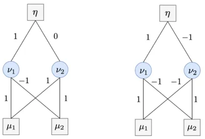
We first define a neural network using the formalism of graph theory to disentangle the architecture from the values of the weights. Unless mention of the contrary, we consider networks with ReLU non-linearities defined as 𝜎(𝑥) = max(𝑥, 0) for 𝑥 ∈ R.
Architecture
A neural network architecture can be represented as a particular directed acyclic graph 𝐺 = (𝑉, 𝐸). We denote a neuron by 𝜈 ∈ 𝑉 and a connection by 𝑒 = 𝜈 → 𝜇 ∈ 𝐸. Each neuron 𝜈 belongs to a layer ℓ(𝜈) ∈J0, 𝐿K.
∙ If ℓ(𝜈) = 0 then 𝜈 belongs to the input layer.
∙ If 0 < ℓ(𝜈) < 𝐿 then 𝜈 belongs to one of the 𝐿 − 1 hidden layers. ∙ If ℓ(𝜈) = 𝐿 then 𝜈 belongs to the output layer.
𝐺 is such that two connected neurons necessarily belong to consecutive layers. We denote 𝐻 ⊂ 𝑉 the set of all hidden neurons. Note that two neurons 𝜇 and 𝜈 in consecutive layers may be connected or not. We denote the neurons of layer ℓ by 𝑁ℓ , {𝜈 | ℓ(𝜈) = ℓ}.
A full path 𝑝 is a sequence of connected neurons 𝑝 = (𝜈0, . . . , 𝜈𝐿) where 𝜈ℓ ∈ 𝑁ℓ,
0 ≤ ℓ ≤ 𝐿 and 𝜈ℓ−1 → 𝜈ℓ ∈ 𝐸 for 1 ≤ ℓ ≤ 𝐿. We say that a connection 𝑒 belongs
to 𝑝 = (𝜈0, . . . , 𝜈𝐿) if there exists ℓ such that 𝑒 = 𝜈ℓ−1 → 𝜈ℓ. We may write 𝑝 ∩ 𝐻
to denote the hidden neurons (𝜈1, . . . , 𝜈𝐿−1) belonging to the path 𝑝. We denote by
𝒫(𝐺) the set of all full paths connecting some input neuron to some output neuron. We also define a partial path 𝑞 = (𝜈ℓ, . . . , 𝜈𝐿) as a sequence of connected neurons
between any hidden layer ℓ with 0 ≤ ℓ ≤ 𝐿 and the output layer. We finally denote by path segment a sequence of connected neurons (𝜈ℓ, . . . , 𝜈ℓ′) where 0 ≤ ℓ ≤ 𝐿 and
0 ≤ ℓ′ ≤ 𝐿. We denote 𝒬(𝐺) the set of such partial paths and we have 𝒫(𝐺) ⊂ 𝒬(𝐺). We may omit the dependency of the underlying graph 𝐺 when it is obvious and simply write 𝒫 and 𝒬. We may simply denote full paths by paths when the context is clear.
For any neuron 𝜈, we define
prev(𝜈) , {𝜇 ∈ 𝑉 | 𝜇 → 𝜈 ∈ 𝐸} next(𝜈) , {𝜇 ∈ 𝑉 | 𝜈 → 𝜇 ∈ 𝐸}
(1) (2)
and for a set of neurons 𝑉 , prev(𝑉 ) = ∪𝜈∈𝑉 prev(𝜈). We denote by Parents(𝜈) the
set of all parent neurons of 𝜈
Parents(𝜈) ,⋃︁
ℓ
prevℓ({𝜈}) (3)
where prevℓ denotes the composition of the operator prev with itself. We similarly define Children(𝜈) the set of all children neurons of 𝜈. We also introduce the notation ∙ → 𝜈 to denote any edge 𝑒 ∈ 𝐸 that has the form 𝜇 → 𝜈 for some 𝜇 ∈ prev(𝜈) and similarly for the notation 𝜈 → ∙.
Weights and Biases
Throughout the manuscript, we will manipulate quantities involving the weights and biases of the network, and find it cleaner to index them all using the connections of the network or its neurons. The graph 𝐺 = (𝑉, 𝐸) is valued with the weights of the network. The weights can be represented:
∙ At the connection level by 𝑤𝑒 ∈ R with 𝑒 ∈ 𝐸;
∙ At the layer level by 𝑊(ℓ) ∈ R𝑁ℓ−1×𝑁ℓ where 𝑊(ℓ) = (𝑤
𝜈→𝜇)𝜈,𝜇∈𝑁ℓ−1×𝑁ℓ and
ℓ ∈J1, 𝐿K;
∙ At the network level by 𝑤 ∈ R𝐸.
In order to define weights at the layer level, we write by convention 𝑤𝜈→𝜇 = 0 if
𝜈 → 𝜇 /∈ 𝐸. Besides, given a fixed architecture 𝐺, we allow the case where some
weights 𝑤𝑒, 𝑒 ∈ 𝐸 are zero. Similarly to the weights, the biases can be represented:
∙ At the neuron level by 𝑏𝜈 ∈ R for any hidden neuron 𝜈 ∈ 𝐻 ∪ 𝑁𝐿;
∙ At the layer level by 𝑏(ℓ)
∈ R𝑁ℓ where 𝑏(ℓ) = (𝑏
𝜈)𝜈∈𝑁ℓ and ℓ ∈ J1, 𝐿K; ∙ At the network level by 𝑏 ∈ R𝐻∪𝑁𝐿.
We denote the global network parameterization by 𝜃 = (𝑤, 𝑏) and refer to elements of 𝜃 as parameters of the network. Networks with at least one hidden layer are such that 𝐿 ≥ 2. The case 𝐿 = 1 corresponds to a linear layer without any non-linearity. Note that a network has 𝐿 affine layers and 𝐿 − 1 hidden layers. Finally, we define useful support and sign sets as follows:
supp(𝑤) , {𝑒 ∈ 𝐸 | 𝑤𝑒 ̸= 0} ⊂ 𝐸
supp(𝑏) , {𝜈 ∈ 𝐻 ∩ 𝑁𝐿| 𝑏𝜈 ̸= 0} ⊂ 𝐻 ∩ 𝑁𝐿
We further define the extended sign operator as follows. For 𝑥 ∈ R, sign(𝑥) = 1 if 𝑥 > 0, sign(𝑥) = 0 if 𝑥 = 0 and sign(𝑥) = −1 if 𝑥 < 0. When applied to a vector or a matrix, sign is taken pointwise. We finally define
Sign𝑤 , {𝑤′ ∈ R𝐸 | sign(𝑤′) = sign(𝑤)} Supp𝑤 , {𝑤′ ∈ R𝐸 | supp(𝑤′) ⊆ supp(𝑤)}
Similarly, we define Sign𝑏 and Supp𝑏 and denote Sign𝜃 , Sign𝑤× Sign𝑏 and we denote Supp𝜃 , Supp𝑤× Supp𝑏
Function
We will also need to manipulate the output function or intermediary functions imple-mented by the network. Let 𝐺 be a fixed architecture 𝐺 valued with 𝜃. Recall that we denote by 𝜎 the ReLU non-linearity. We define:
∙ Layer-wise functions. A neural network can be recursively implemented using intermediary row vector functions 𝑦(ℓ)(𝜃) : R𝑁0 → R𝑁ℓ for ℓ ∈
J0, 𝐿K. We define 𝑦(0)(𝜃, 𝑥) = 𝑥 and, for ℓ ∈
J1, 𝐿 − 1K,
𝑦(ℓ)(𝜃, 𝑥) = 𝜎(︁𝑦(ℓ−1)(𝑥)𝑊(ℓ)+ 𝑏(ℓ))︁. (4)
∙ Output functions. The function implemented by the whole network is
𝑦(𝐿)(𝜃, 𝑥) = 𝑦(𝐿−1)(𝜃, 𝑥)𝑊(𝐿)+ 𝑏(𝐿) (5) i.e. the last layer is an affine function of the previous one. We use the notation 𝑅𝐺|𝜃 = 𝑦(𝐿)(𝜃) and we call 𝑅𝐺|𝜃 the realization of the network architecture
𝐺 given the parameters 𝜃. We write 𝑅𝐺|𝜃(𝑥) to denote the evaluation of the
defined function at any input 𝑥 ∈ R𝑁0. When the dependency on the graph 𝐺
is obvious, we may simply write 𝑅𝜃 and 𝑅𝜃(𝑥). With a slight abuse of notation
and for the sake of clarity, we may also write 𝑅(𝜃, 𝑥).
∙ Neuron functions. Given a neuron 𝜈 belonging to layer ℓ, we denote the function implemented by 𝜈 before the non-linearity as 𝑦𝜈(𝜃) : R𝑁0 → R such that
𝑦𝜈(𝜃) = 𝑦(ℓ)𝜈 (𝜃). (6)
and 𝜃′ are functionally equivalent if the realizations 𝑅𝜃 and 𝑅𝜃′ are the same, i.e., if
for all 𝑥 ∈ 𝑅𝑁0, 𝑅
𝜃(𝑥) = 𝑅𝜃′(𝑥).
Useful Quantities
We denote the value of a full path by 𝑣𝑝(𝜃) = 𝑤𝜈0→𝜈1. . . 𝑤𝜈𝐿−1→𝜈𝐿 and we define the
activation status of a full path 𝑝 given the parameters 𝜃 and the input 𝑥 as
𝑎𝑝(𝜃, 𝑥) , ∏︁ 𝜈∈𝑝∩𝐻
1(𝑦𝜈(𝜃, 𝑥) > 0). (7)
We naturally extend the notion of partial path value and the notion of partial path activation status. As the value of a full or partial path only depends on the weights 𝑤 and not on the biases, we may write indifferently 𝑣𝑝(𝜃) or 𝑣𝑝(𝑤) for any full or partial
path. For any path segments 𝑞 = (𝜈ℓ, . . . , 𝜈ℓ′), 𝑞′ = (𝜇ℓ′, . . . , 𝜇ℓ′′) such that 𝜈ℓ′ = 𝜇ℓ′,
we denote the concatenation of 𝑞 and 𝑞′ as 𝑞 + 𝑞′ = (𝜈ℓ, . . . , 𝜈ℓ′, 𝜇ℓ′+1, . . . , 𝜇ℓ′′).
Algebraic Tools
We will rely on algebraic and geometric interpretation to understand the action of rescaling operations on a parameterization 𝜃. To this end, we represent the mapping between edges and paths by the linear operator P : R𝐸 → R𝒫 such that for every connection 𝑒 ∈ 𝐸 and every path 𝑝 ∈ 𝒫,
(P𝛿𝑒)𝑝 , ⎧ ⎨ ⎩ 1 if 𝑒 ∈ 𝑝 0 otherwise (8)
where 𝛿𝑒 ∈ R𝐸 is the dirac vector for edge 𝑒. We denote by 𝒟(𝑁 ) the set of diagonal
matrices 𝐷 ∈ R𝑁 ×𝑁 such that, for all 𝑖, 𝑑
𝑖 = 𝐷𝑖,𝑖 is strictly positive.
Admissible parameterizations
We say that the network parameterization 𝜃 = (𝑤, 𝑏) is admissible if, for every hidden neuron 𝜈 ∈ 𝐻, there exists a full path 𝑝 ∈ 𝒫 going through 𝜈 such that 𝑣𝑝(𝜃) > 0.
Equivalently, every hidden neuron 𝜈 ∈ 𝐻 is connected to some input and some output neuron through a path with non-zero weights. As the notion of admissibility only depends on the weights 𝑤 and not on the biases 𝑏, we may indifferently mention an admissible parameterization or admissible weights.
Chapter 1
Introduction
Computer Science has shaped our modern society in a tremendous way, in part since the seminal work of Alan Turing, who invented an abstract computer called the Turing Machine in 1936. Since then, this concept has materialized in the form of processors and chips with an extremely wide range of applications. In a fast-paced search for performance, the building blocks of modern computers called transistors have become smaller and smaller according to Moore’s law, which states that the number of transistors on a chip doubles after a short, constant period of time1. Thanks to this miniaturization, the ubiquity of interconnected portable computers, prophesied by Silicon Valley entrepreneurs (Gates and Ottavino, 1995) or even by french writer Marguerite Duras2 in 1985 is now a reality.
Such powerful and portable devices, including smartphones or virtual/augmented reality headsets, constitute a fertile ground for a particular class of algorithms called Deep Neural Networks (DNNs). These models are programmed to learn to perform specific tasks – hence the name Deep Learning – and belong to the more general field of Artificial Intelligence, also pioneered by Turing3. While DNNs are increasingly powerful for detecting persons in images or understanding and translating speech or text for instance, they still lack efficiency in terms of size and speed.
Hence, after the miniaturization of the computers themselves, the miniaturization or compression of DNNs is now a key challenge to deploy them on-device and in real
1Every 18 or 24 months according to a majority of the estimates. However, it is uncertain that
this empirical law will hold in the future: with a characteristic scale of 5 nanometers of 2020 down to 3 and 2 nanometers in the next years, the transistors are now so small that they begin to experience quantum tunneling effects perturbing their functioning.
2https://www.ina.fr/video/I04275518, television interview in French by Michel Drucker. 3The Turing Award, usually considered as the highest distinction in Computer Science, was
awarded to Yoshua Bengio, Geoffrey Hinton, and Yann LeCun in 2018 for their “conceptual and engineering breakthroughs that have made deep neural networks a critical component of computing”.
time. It would offload the servers that currently run such models, reduce the latency and promote more privacy since personal data would be analyzed directly on-device. This is particularly relevant after the European Union’s new data privacy and security law entered into force in 2016, the General Data Protection Regulation (GDPR)4.
In this Chapter, we first detail the general topics of efficiency and redundancy in deep learning and the underlying reasons motivating our work in Section 1.1. We then briefly summarize the interesting challenges that the Deep Learning community is facing on these areas in Section 1.2 and finally detail our contributions, both academic and product-oriented and the general organization of the manuscript in Section 1.3.
1.1
Motivation
We summarize here the main reasons that conducted us to study the redundancy and efficiency of Neural Networks both theoretically and in practice.
The Deep Learning Revolution. Following pioneering work by Rumelhart et al. (1986), LeCun et al. (1989) or (LeCun et al., 1998b), the inception of AlexNet by Krizhevsky et al. (2012) marked a turning point in the development of Deep Learn-ing. Back in 2012, a heavy neural network, trained with stochastic gradient descent (SGD) and properly regularized, surpassed all existing methods by a large margin on the ImageNet competition (Deng et al., 2009). Since then, the concept of “Ima-geNet moment” was transposed to various domains where Deep Learning percolated with an unreasonable effectiveness, from Natural Language Processing (Ruder, 2019) a few years ago to protein folding as we write these lines (Jumper et al., 2020). Strong empirical evidence of deep learning approaches was also shown for extremely various tasks such as symbolic mathematics (Lample and Charton, 2019), fast MRI reconstruction (Zbontar et al., 2018) or quantum physics (Sch¨utt et al., 2017).
Bigger, Hence Better Models. Fueled by this tremendous success on numerous tasks, a fast-paced search for performance is occurring in the research community. Since one straightforward way to improve expressivity – hence performance – is to act on depth by stacking more layers (Telgarsky, 2016; Raghu et al., 2017), researchers are considering the biggest possible networks they can train (Simonyan and Zisserman, 2014; He et al., 2015b), now up to 175 billion parameters (Rajbhandari et al., 2020;
4
https://gdpr-info.eu/. It is a substantial update of the European Data Protection Directive passed in 1995 by the EU.
Rasley et al., 2020; Brown et al., 2020). Training such networks requires huge amounts of data (labelled or not), energy and performant distributed computing infrastructure relying on GPGPUs or TPUs5.
Redundancy and Efficiency in Deep Learning Models. Then, as the research community produces bigger networks, the question of their redundancy and efficiency naturally arises in order to manipulate such networks more easily. Roughly speaking,
redundancy6 refers to a certain structure in the parameters of a neural network where
some weights or groups of weights carry similar information (LeCun et al., 1990; Denil et al., 2013). On the other hand, efficiency7 refers to Pareto efficiency (Fudenberg and Tirole, 1991) of a model given set of metrics8, traditionally in terms of model size, model accuracy and inference time (Wang et al., 2018a). Thus, studying redundancy in deep learning models may help improve their efficiency, at least on the model size axis. Note that various setups – especially in terms of hardware – and constraints on these metrics may lead to distinct Pareto optima.
Making the Best Models Available to Everyone. Studying redundancy in deep learning to produce more efficient models is thus crucial for deploying the best models both on servers and on mobile devices. On the server side, the objective is to produce more parsimonious models in terms of parameters (Radosavovic et al., 2020; Tan and Le, 2019) or training data (Touvron et al., 2020), which may lead to a faster training time9 , energy savings, or help consider even bigger models to train. On the mobile side, deploying models on embedded devices such as smartphones, autonomous vehicles or virtual/augmented reality headsets10 opens up to numerous applications. Having such models on-device instead of performing the inference on a remote server reduces the latency and the network congestion, works offline and is compatible with privacy-preserving machine learning where the data stays on the user’s device (Knott et al., 2020), at the cost of exposing the embedded model to various attacks. It also enables federated learning (Koneˇcn´y et al., 2017) where a centralized model is trained while training data remains distributed over a large number of client devices with unreliable network connections.
5Respectively General Purpose Graphics Processing Units and Tensor Processing Units. 6More details in Sections 2.1 and 2.2.
7More details in Section 2.3.
8Such metrics are not independent: larger models are generally more accurate but slower. 9For instance, AlphaGo (Silver et al., 2017) took 40 days to train on a vast infrastructure. 10Such as Oculus Quest 2 for VR (Virtual Reality) or HoloLens 2 for AR (Augmented Reality).
1.2
Challenges
Redundancy is intimately related to the concept of over-parameterization, which is a key characteristic of modern neural networks (Srivastava et al., 2014) – see Subsection 2.1.1 for definitions and discussions. Over-parameterized networks have a high ability to fit training data, yet they are challenging to train, they are difficult to comprehend from a theoretical point of view and they pose significant hurdles to real-time appli-cations on embedded devices. We briefly summarize these challenges in this Section and refer the reader to Chapter 2 for a more extensive discussion.
Theoretical Considerations on Redundancy. Parameter redundancy of deep learning models is a well-known fact (Denil et al., 2013) and has clear drawbacks – first and foremost, the model size. However, reducing this redundancy is challenging and indirectly provides hints on the benefits of redundant, over-parameterized models. At training time, researchers study the interplay between over-parameterization and SGD (Li and Liang, 2018; Sankararaman et al., 2019) to help mitigate overfitting. Taking advantage of this redundancy may lead to more efficient or performant training procedures. For instance, grouping networks that behave similarly and implicitly performing SGD in a reduced or quotiented space may help, see Chapters 3 and 4.
Redundancy in Practice for Efficient DNNs. While training happens once, the trained model is subsequently used numerous times for inference. For instance, at Facebook, deep learning models analyze trillions of bits of content per day. Then, the challenge is to compress the network – or more generally, to make it more efficient – without losing too much predictive performance or accuracy, sometimes referred to as the size/accuracy tradeoff, see Chapters 5 and 6. Another challenge is to select the best compression algorithm – or combination thereof – among a large set of methods that are not entirely orthogonal, given a target size/accuracy tradeoff. For instance, is it better to compress a large, high-performing network instead of a mobile-efficient architecture that is smaller but has a slightly degraded predictive performance?
On-device and Real Time Deployment. While less redundant networks are generally faster at inference, redundancy is only a part of the story. Indeed, compres-sion algorithms with an excellent comprescompres-sion ratio could necessitate to decompress the network before inference instead of performing the prediction in the compressed domain. Hence, a good compression algorithm also depends on the task and hardware constraints – generally, inference has to be performed in real-time without draining
the battery and overloading the RAM11, see Chapter 7. This involves low-level con-siderations on the type of hardware used for inference, see Subsection 2.3.6 for details.
1.3
Contributions
We detail the general organization of the manuscript and then enumerate our aca-demic contributions as well as the applications and technology transfers derived di-rectly from our published papers.
1.3.1
Outline
We present here our contributions in ascending order of applicability, measured as the closeness to production. We first start by presenting theoretical contributions on functional equivalence classes, then explore the compression of deep learning models down to the on-device deployment of such efficient models.
Equivalence Classes of Neural Networks. In Chapter 3, we study functional equivalence classes of ReLU neural networks. We first show that such classes contain orbits generated by the action of rescalings and permutations of hidden neurons for networks with arbitrary depth. We then characterize functional equivalence classes for one-hidden-layer networks under some non-degeneracy conditions and investigate the case with many hidden layers by designing algebraic tools to study the problem locally. Leveraging these theoretical considerations, we develop an alternative to the Stochastic Gradient Descent (SGD) algorithm in Chapter 4. Our variant, called Equi-Normalization or ENorm, alternates between standard SGD steps and balancing steps amounting to change the representant of the current functional equivalence class by selecting the one that minimizes a given energy function. Balancing steps preserve the output – hence the accuracy – of the network by definition but modify the gradients of the next SGD step, hence the learning trajectory. In other words, ENorm takes advantage of the redundancy in the parameter space by operating the optimization in the quotient space induced by the functional equivalence relation.
Neural Network Compression. Studying the redundancy of the network’s pa-rameters in the first part of the thesis naturally leads to the question of the efficiency
of such networks, hence to the question of their compression. In Chapter 5, we de-velop a novel method, called Iterative Product Quantization or iPQ, that relies on vector quantization in order to drastically reduce the size of a network while almost preserving its accuracy. The proposed approach iteratively quantizes the layers and then finetunes them. The quantization step is performed by splitting the layer’s weight matrix into a set of vectors that are clustered into a common codebook. In order to boost the obtained size/accuracy tradeoffs, we develop a pre-conditioning method that injects carefully selected quantization noise when training the network before its compression. The method, called Quant-Noise, is described in Chapter 6 and has proven to be effective for both iPQ and for traditional scalar quantization such as int8 or int4. Quant-Noise is effective for a variety of tasks and quantization methods and thus reconciles pre-training for both scalar and vector quantization.
Ultra-Low Bandwidth Generative Video Chat. While the compressed size of the network is a significant indicator of the quality of the quantization, other metrics such as inference time and battery usage are also relevant, especially for on-device, real time applications. Hence, we investigated potential applications for iPQ and Quant-Noise. Among them, we design a method, called FaceGen, to perform ultra-low bandwidth video chats in Chapter 7. FaceGen streams compressed facial landmarks from the sender’s phone to the receiver, and uses a generative adversarial network to reconstruct the sender’s face based on the stream of landmarks plus one identity embedding sent once at the beginning of the call. The stream of landmarks is compressed to less than 10 kbits/s, and the networks are quantized to a total size of less than 2 MB and run at 20+ frames per second on an iPhone 8.
1.3.2
Publications
The work presented in this manuscript was also published in the following papers, that were written during the thesis.
∙ Pierre Stock, Benjamin Graham, R´emi Gribonval and Herv´e J´egou. Equi-normalization of Neural Networks. Published at ICLR 2019 (Stock et al., 2019a). Source code: https://github.com/facebookresearch/enorm.
∙ Pierre Stock, Armand Joulin, R´emi Gribonval, Benjamin Graham and Herv´e J´egou. And the Bit Goes Down: Revisiting the Quantization of Neural Net-works. Published at ICLR 2020 (Stock et al., 2019b). Source code: https: //github.com/facebookresearch/kill-the-bits.
∙ Pierre Stock*, Angela Fan*, Benjamin Graham, Edouard Grave, R´emi Gribon-val, Herv´e J´egou and Armand Joulin. Training with Quantization Noise for Ex-treme Model Compression. Published at ICLR 2021 (Stock et al., 2020). Source code: https://github.com/pytorch/fairseq/tree/master/examples/quant_ noise
∙ Maxime Oquab*, Pierre Stock*, Oran Gafni, Daniel Haziza, Tao Xu, Peizhao Zhang, Onur Celebi, Yana Hasson, Patrick Labatut, Bobo Bose-Kolanu, Thibault Peyronel, Camille Couprie. Low Bandwidth Video-Chat Compression using Deep Generative Models. Under review, 2021 (Oquab et al., 2020).
The following paper was written during an internship at Facebook AI Research and will not be discussed in this manuscript.
∙ Pierre Stock, Moustapha Cisse. ConvNets and ImageNet Beyond Accuracy: Explanations, Bias Detection, Adversarial Examples and Model Criticism. Pub-lished at ECCV 2018 (Stock and Cisse, 2018).
1.3.3
Technology Transfers
The research presented in this manuscript led to various technology transfers, which are briefly summarized here. Seeking for internal applications and collaborations and delivering product impact was the main focus of the last year of my PhD.
∙ The iPQ technique described in Chapter 5 is currently used to design fast CPU kernels for quantized models for both server side and mobile side, relying on the fbgemm12 library for quantized matrix multiplication.
∙ The pre-conditioning technique Quant-Noise (Chapter 6) was used to deploy a quantized int8 model for internal dogfooding. The model aims at detecting harmful content in conversations on-device on real time.
∙ The low-bandwidth generative video chat method described in Chapter 7 is cur-rently under productionization and led to a US patent application P201451US00.
12
Chapter 2
Related Work
In this Chapter, we review the lines of work addressing the question of parameter redundancy and efficiency in Deep Learning. In Section 2.1, we first discuss the ben-efits of depth for neural networks in terms of expressivity and capacity to fit training data. We enumerate the main practical training challenges along with the methods and tools to mitigate them, in particular in terms of normalization layers. This line of work is related to our contribution in Chapter 4, where we re-normalize the network’s weights after each training step while preserving the function implemented by the network. Then, we review the theoretical studies aiming at characterizing functional equivalence classes of neural networks in Section 2.2. Such equivalence classes allow to aggregate networks that behave identically to only manipulate one representant per class, thus effectively operating in the quotient space. This work is related to our contribution detailed in Chapter 3 and shows that under some assumptions, the equivalence classes only encompass permutations and rescalings of neurons (see 2.2.1). Finally, we study network compression in Section 2.3. We review the methods aiming at reducing the redundancy in the set of the network’s parameters while maintaining a competitive accuracy and inference speed, in particular scalar and vector quantiza-tion. This section is related to our contributions on Iterative Product Quantization and Quantization Noise that are detailed in Chapters 5 and 6. More specifically, the subsection about on-device deployment is related to our Ultra-low Bandwidth Generative Video Chat contribution detailed in Chapter 7.
2.1
Over-Parameterization: a Double-Edged Sword
The inception of AlexNet (Krizhevsky et al., 2012) demonstrated that a deep neural network surpassed existing computer vision techniques by a good margin1 on the Im-ageNet classification task (Deng et al., 2009). This success is conditioned on proper training techniques, the availability of large datasets, as well as huge computing ca-pabilities. Since then, a part of the research community has focused on scaling the architectures, the datasets and the training techniques in the search of better per-formance (Brown et al., 2020). This fast-paced practical search for deeper networks, followed by a more theoretical analysis of the benefits of depth, is reviewed in Subsec-tion 2.1.1. Then, we briefly enumerate the training challenges posed by such networks in Subsection 2.1.2 along with the tools to mitigate them in Subsection 2.1.3, including various normalization layers. Subsections 2.1.1 and 2.1.2 do not aim to be exhaustive but act rather as motivating illustrations for the remainder of this chapter.
2.1.1
With Greater Depth Comes Greater Expressivity
We briefly review and discuss the notion of over-parameterization, followed by a more theoretical analysis of the benefits of depth in terms of expressivity. Here, we do not aim at a comprehensive review but rather focus on a few illustrative examples.
Over-parameterization
Over-parameterized networks are primarily characterized by their large number of parameters2 with respect to the number of training samples in the Deep Learning literature (Sagun et al., 2018; Allen-Zhu et al., 2019; Li and Liang, 2018). For in-stance, AlexNet has 60 million parameters, which is an order of magnitude larger than 1.2 million train images of ImageNet (Deng et al., 2009). Note that a more rigorous definition would take into account various factors such as the sample size3, the architecture 𝐺 or even the data itself (Sagun et al., 2018).
Next, we briefly focus on a few illustrative examples acknowledging the parameter redundancy in neural networks in practice. First, the fact that some parameters can
1The ILSVRC-2012 test top-5 error rate was 15.3% for AlexNet compared to 26.2% for the second
best entry of the competition.
2The number of parameters of a neural network with architecture 𝐺 is the number of connections
in 𝐺 (except for the biases). Sometimes authors consider the number of neurons rather than the number of connections (Gribonval et al., 2019).
3Fitting 𝑁 training samples in a low dimension input space would require less parameters than
be deleted or pruned without harming the accuracy is well-known (LeCun et al., 1990), as discussed in Subsection 2.3.1. More recently, Denil et al. (2013) demonstrate that there is a significant redundancy in the network parameters of several deep learning models by accurately predicting 95% of the parameters based only on the remaining 5%, with a minor drop in accuracy. The motivation behind this technique is the fact that the first layer features of a convolutional neural network trained in natural images (e.g. ImageNet (Deng et al., 2009)) tend to be locally smooth with local edge features, similar to local Gabor filters4. Given this structure, representing the value of each pixel separately is redundant as the value of one pixel is highly correlated with its neighbors. Denil et al. (2013) propose to take advantage of this type of structure to factor the weight matrix. Similar approaches that learn a basis of low-rank filters are explored by Jaderberg et al. (2014).
Depth and Expressivity
The relation between the network’s depth and its expressivity is widely studied (Pas-canu et al., 2013; Mont´ufar et al., 2014; Eldan and Shamir, 2015; Telgarsky, 2016; Raghu et al., 2017; Gribonval et al., 2019). For instance, Mont´ufar et al. (2014) study the number of linear regions defined by a given architecture. As defined more for-mally in Subsection 2.2.2 in the case of ReLU networks, linear regions are the areas of the input space on which the gradient of the function implemented by the network ∇𝑥𝑅𝜃 is constant. The number of linear regions is connected to the complexity of the
function implemented by the network: more linear regions means that the network is able to fit more complex training data. The authors derive a lower bound on the maximal number of linear regions and show in particular that, for architectures with fixed widths, the maximal number of linear regions – hence the expressivity of the network – grows exponentially in the number of layers.
While the expressivity of a network somehow grows exponentially with its depth, another approach to obtain a network with the same number of parameters is to increase its width when keeping the number of layers fixed. This strategy generally results in less expressive networks, as shown by Eldan and Shamir (2015). The authors exhibit a simple radial function 𝜙 in R𝑑 that is implementable by a two-hidden-layer
network but cannot be tightly approximated by any one-hidden-layer network, unless its width grows exponentially in the input dimension 𝑑. The authors conclude that “depth can be exponentially more valuable than width” for feedforward networks.
Figure 2-1: The double-descent phenomenon in Deep Learning as illustrated by Nakki-ran et al. (2019). Here the complexity of the considered model (a ResNet-18) is mea-sured as its width parameter, where higher width denotes a network with a larger number of parameters.
2.1.2
Deeper Networks Present Harder Training Challenges
In this Subsection, we briefly review the main training challenges of neural networks that arise as the networks go deeper in the search for more and more expressivity, as mentioned in Subsection 2.1.1. We refer the reader to the cited work below for a more exhaustive overview.
Overfitting
Overfitting is traditionally approached in Machine Learning through the Bias-Variance trade-off, as explained for instance by Hastie et al. (2009). According to this prin-ciple, as the model complexity – measured with its number of parameters or with more elaborate tools such as the VC dimension (Vapnik, 1998) or the Rademacher complexity (Bartlett and Mendelson, 2003) – increases, the training error decreases while the test error follows a U-shaped curve. Models with low complexity underfit and suffer from high bias whereas models with high complexity exhibit a high vari-ance, suggesting that an intermediate model complexity reaches the optimal trade-off. However, recent work by Belkin et al. (2018), followed by Nakkiran et al. (2019); Mei and Montanari (2019); d’Ascoli et al. (2020) uncovered a double-descent behavior for deep learning models. After a critical regime, the test error goes down again as illus-trated in Figure 2-1. This finding is consistent across architectures, optimizers and tasks (Nakkiran et al., 2019), suggesting, as found in practice, that deeper models and more data lead to better performance (Krizhevsky et al., 2012).
As stated before, given a fixed training dataset, overfitting is traditionally mea-sured using the number of parameters of the considered model. In the search for more elaborate model complexity measures, Zhang et al. (2016) propose a protocol
Figure 2-2: Fitting random labels and random pixels on CIFAR10 as illustrated by Zhang et al. (2016).
for understanding the effective capacity of machine learning models. The authors train several architectures on a copy of the training data where either (1) the orig-inal labels were replaced by random labels; or (2) the pixels were shuffled; or (3) the pixels were drawn randomly from gaussian noise. They observe that the train-ing error goes down to zero provided that the number of epochs is large enough, as depicted in Figure 2-2, and conclude that “deep neural networks easily fit random labels”. Or course, if the amount of randomization is larger, the time taken to overfit is longer. Such work paves the way for more formal complexity measures to explain the generalization ability of neural networks.
Vanishing and Exploding Gradients
In the 90’s, feedforward neural networks – convolutional or fully connected – were a few layers deep (LeCun et al., 1989) and were trained through back-propagation. However, Bengio et al. (1994) reported difficulties to train recurrent networks in order to learn long-term dependencies – for instance in a sequence of words. The principle of recurrent networks is to apply the same weight matrix iteratively on the input sequence while updating a hidden state. Recurrent networks are usually trained with back-propagation through time (BPTT, Williams and Zipser (1995); Rumelhart et al. (1986); Werbos (1988)), where the network is unfolded for a fixed sequence length and trained using standard back-propagation. When working on an improved version of recurrent networks named LSTMs (Long Short-Term Memory networks, Hochreiter and Schmidhuber (1997)), Hochreiter and Bengio (2001) identify two undesirable behaviors of the gradients flowing backward in time: such gradients either blow up or vanish, resulting in training instabilities.
As feedforward networks went deeper, similar vanishing or exploding gradient problems arise Mishkin and Matas (2016) He et al. (2015c). Such training instabili-ties were related in part to the magnitude of the weights. The research community proposed tools to mitigate this undesirable training behavior as explained in Subsec-tion 2.1.3. Failure modes preventing the training from properly starting were also theoretically studied by Hanin (2018).
2.1.3
The Deep Learning Training Toolbox
The training challenges of deep neural networks mentioned in Subsection 2.1.2 are overcome by various methods designed along the years. We briefly enumerate the main strategies that constitute the toolbox of every researcher and practitioner, in particular in terms of normalization layers. This line of work is related to our contri-bution detailed in Chapter 4.
Initialization Schemes
Properly initializing the weights of a neural network before training it alleviates the vanishing or exploding gradient problem in the first training iterations and allows stochastic gradient descent algorithms to find a suitable minimum, starting from this initialization. By studying the distribution of activations and gradients, Glorot and Bengio (2010) designed an initialization scheme to preserve the variance of activations and gradients across layers for networks with symmetrical activation functions like the sigmoid or the hyperbolic tangent. Following this idea, (Mishkin and Matas, 2016) and He et al. (2015c) designed initialization schemes for networks with Rectified Linear Units (ReLUs). This leads to a popular weight initialization technique
𝑊ℓ ∼ 𝒩
(︂
0,√︁2/𝑁ℓ−1 )︂
where 𝑁ℓ−1 is the number of input features5. Finally, failure modes that prevent the
training from starting have been theoretically studied by Hanin and Rolnick (2018).
Data Augmentation
Data augmentation is widely used to easily generate additional data to improve ma-chine learning systems in various areas (Krizhevsky et al., 2012; Huang et al., 2016; Wu et al., 2019c) and to reduce overfitting. Traditionally, for object classification, at
5For convolutions, 𝑁
training time, a random resized crop6 is applied to the image which is then flipped horizontally with a probability 0.5. Since then, many more augmentation techniques were designed. For instance, Zhang et al. (2017a) train a network on convex combina-tions of pairs of examples and their labels, while (Cubuk et al., 2018) automatically search for improved data augmentation policies with a method called AutoAugment. We refer the reader to Cubuk et al. (2019) for a survey of data augmentation tech-niques. On a side note, the random resized crops used at training time involve a rescaling of the input image, in contrast to the center crops used at test time. Thus, the network is generally presented with larger objects at training time than at test time. This train-test resolution discrepancy is addressed by (Touvron et al., 2019) with a method called FixResNets.
Architectures
As networks are getting deeper, two major architectural changes are introduced to prevent the gradients to vanish. Rectified Linear Units (ReLUs) defined as 𝜎(𝑥) = max(0, 𝑥) are applied pointwise on the activations. Krizhevsky et al. (2012) were among the first to successfully employ such non-saturating activation functions to Convolutional Neural Networks, as opposed to traditional saturating functions like the sigmoid. Moreover, to allow the information to flow better up and down the network, He et al. (2015a) introduced skip-connections between blocks. More formally, if 𝑓 is a building block7, adding a skip connection amounts to output 𝑓 (𝑥) + 𝑥 after the block instead of 𝑓 (𝑥) for any input activation 𝑥. Skip connections are now ubiquitous in deep learning architectures such as the Transformers in NLP (Vaswani et al., 2017).
Optimization
Neural networks are originally trained with Stochastic Gradient Descent (SGD)8, generally with momentum LeCun et al. (1989). Denoting 𝜃𝑡 the parameters at time
step 𝑡 and ℒ the loss function, one possible set of equations for SGD writes9:
⎧ ⎨ ⎩
𝜃𝑡+1 = 𝜃𝑡− 𝜂𝑣𝑡+1
𝑣𝑡+1 = 𝜇𝑣𝑡+ ∇𝜃ℒ
6The input image is cropped with a random size and a random aspect ratio, and finally resized
to the input size.
7For instance, two convolutions interleaved with one ReLU.
8Iterating over mini-batches of data, not single elements of the train set.
9There is also a Nesterov version (Nesterov, 1983) as well as the possibility to apply the learning
where 𝜂 is the learning rate and 𝜇 the momentum coefficient, generally set to 0.9. This remains the main training recipe for Image Classification problems (Goyal et al., 2017; Wu and He, 2018). The learning rate is generally following a schedule, meaning that 𝜂 = 𝜂𝑡 depends on the current epoch or iteration. A classical schedule starts
with a warm-up phase followed by a decay phase10 (He et al., 2015a). Interestingly, the cosine schedule is gaining traction both in Vision and in NLP (Radosavovic et al., 2020). However, choosing a proper learning rate along with its schedule is expensive. Therefore, Duchi et al. (2011) designed a first-order gradient method named Adagrad that accounts for the anisotropic relation between the network’s parameters and the loss function. More precisely, given a default learning rate 𝜂0 usually set to 0.01 and a small constant for numerical stability 𝜀,
⎧ ⎪ ⎪ ⎨ ⎪ ⎪ ⎩ 𝑤𝑒,𝑡+1= 𝑤𝑒,𝑡− 𝜂0 √ 𝑔𝑒,𝑡+1+ 𝜀 ∇𝑤𝑒ℒ 𝑔2𝑒,𝑡+1= 𝑔2𝑒,𝑡+ (∇𝑤𝑒ℒ) 2 .
In other words, each weight 𝑤𝑒 is updated with an adaptive learning rate that
de-pends on the sum of the past gradients with respect to this weight. Other adaptive algorithms were derived, or instance by Kingma and Ba (2014) which proposed a vari-ant called Adam, frequently used in NLP. Intuitively, whereas SGD with momentum can be seen as a ball running down a surface, Adam behaves like a heavy ball with friction. For information about second-order methods or convergency considerations, we refer the reader to the manuscript by Bottou et al. (2016).
Weight Decay
Weight decay is a regularization method that is widely used in Deep Learning (Krogh and Hertz, 1992). It adds a penalty term to the traditional loss, for instance the cross-entropy loss 𝒞 in image classification. The training loss writes
ℒ = 𝒞 + 𝜆‖𝜃‖2 2
where 𝜃 is the network’s parameters (weights and biases) and 𝜆 an hyper-parameter to cross-validate11. Weight decay is well suited for SGD as it amounts to add a term 2𝜆𝜃 to the gradients computed by back-propagation.
10For instance, given a default value 𝜂
0, use the learning rate 𝜂0/10 during the first 5 epochs
(warm-up). Then, set the learning rate back to 𝜂0and decay it a factor 10 every 30 epochs (decay). 11Generally, 𝜆 = 10−4 or 10−5.
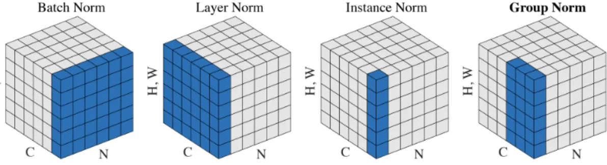
Figure 2-3: The effect of various normalization layers as illlustrated by Wu and He (2018). 𝑁 denotes the batch size, 𝐶 the channel dimension and 𝐻 and 𝑊 the spatial axes. The colored pixels are normalized with the same mean and standard deviation.
Dropout
Dropout (Hinton et al., 2012b) is a technique that randomly drops neurons12, weights or more important structures (Ghiasi et al., 2018) during training time with a fixed small probability 𝑝13. This prevents the network from overfitting given the large variety of internal states it has to operate on. Dropout serves other purposes, for example, it helps pruning entire layers at test time (Fan et al., 2019) and is also related to our Quant-Noise contribution in Chapter 6.
Normalization Layers
Normalization procedures take an important part in the development of neural net-works. While the inputs are almost always preprocessed14 (LeCun et al., 1989), researchers began to normalize inner features as the networks were deeper. After successful attempts on whitening or local response normalization (Krizhevsky et al., 2012), Batch Normalization (BN) (Ioffe and Szegedy, 2015) is now a standard nor-malization layer. Let us detail BN in the context of computer vision. Denote the activations after some layer ℓ in the network by 𝑥 ∈ R𝑁 ×𝐶×𝐻×𝑊, where 𝑁 is the
batch size, 𝐶 the number of channels, 𝐻 and 𝑊 the respective height and width of the activations, sometimes called spatial dimensions. For instance, an input im-age generally has shape 1 × 3 × 224 × 224 for three color channels (RGB) and a size of 224 × 224. For simplicity, we often flatten the last two dimensions so that
𝑥 ∈ R𝑁 ×𝐶×𝐻𝑊 as depicted in Figure 2-3.
12When dropping a neuron 𝜈 ∈ 𝐻 during a training iteration, we set 𝑤
∙→𝜈 = 0 and 𝑤𝜈→∙ = 0 and we do not update 𝑤∙→𝜈 = 0 and 𝑤𝜈→∙ during the backward pass. In other words, we detach all the incoming and outcoming connections of 𝜈 from the forward and backward passes.
13Generally 𝑝 ∈ [0.1, 0.3].
First, BN normalizes 𝑥 per-channel into 𝑥. More formally, denoting 𝑐 ∈̂︀ J1, 𝐶 K a given channel, we have
̂︀
𝑥[:, 𝑐, :, :] = 𝑥[:, 𝑐, :, :] − 𝜇√︁ 𝑐
𝜎2
𝑐 + 𝜀
where 𝜀 is a small constant for numerical stability and where 𝜇𝑐and 𝜎𝑐are the sample
mean and (biased) standard deviation defined as 𝜇𝑐= 1 𝑁 𝐻𝑊 ∑︁ 𝑛,ℎ,𝑤 𝑥[𝑛, 𝑐, ℎ, 𝑤] 𝜎2𝑐 = 1 𝑁 𝐻𝑊 ∑︁ 𝑛,ℎ,𝑤 (𝑥[𝑛, 𝑐, ℎ, 𝑤] − 𝜇𝑐)2
Second, the BN layer learns an affine transform of 𝑥 on the channel dimension:̂︀
𝑦 = 𝛾𝑥 + 𝛽̂︀
where 𝛾 and 𝛽 are learnt parameters of size 𝐶. More formally, for any batch, channel and spatial indexes 𝑛, 𝑐, ℎ, 𝑤, we have
𝑦𝑛,𝑐,ℎ,𝑤 = 𝛾𝑐𝑥̂︀𝑛,𝑐,ℎ,𝑤 + 𝛽𝑐. (2.1)
Since the normalization statistics 𝜇𝑐 and 𝜎𝑐 depend on the batch, at test time BN
is switched to evaluation mode and uses fixed statistics 𝜇𝑐 and 𝜎𝑐 that are estimated
with an exponential moving average of 𝜇𝑐 and 𝜎𝑐 during training time. Thus, at test
time, BN is an affine layer.
While extremely effective in standard setups, Batch Normalization suffers from known shortcomings. In particular, BN only works well with sufficiently large batch sizes (Ioffe and Szegedy, 2015; Wu and He, 2018). For batch sizes below 16 or 32, the batch statistics 𝜇𝑐and 𝜎𝑐have a high variance and the test error increases significantly.
Since then, variants of this technique such as Layer, Instance or Group Normalization (Ba et al., 2016; Ulyanov et al., 2017; Wu and He, 2018) were successfully introduced to circumvent the batch dependency, see Figure 2-3 for an illustration. For instance, Transformers (Vaswani et al., 2017) rely on Layer Normalization whereas Generative Adversarial Networks (GANs) use other variants such as the SPADE block (Park et al., 2019). This line of work is related to our Equi-normalization contribution in Chapter 4 where we re-normalize the weights – not the activations – in order to minimize the global 𝐿2 norm of the network to ease the training.
Hyperparameter Tuning
One of the main difficulties of neural network training lies in finding the proper set of hyperparameter values15 in the high-dimensional space of all the possible aforemen-tioned techniques. For instance, Lample et al. (2017) found it extremely beneficial to add a dropout rate of 0.3 in some part of their architecture and Carion et al. (2020) underline the crucial importance of having two different learning rates for the two main components of their architecture. While the traditional cartesian grid search remains the main investigation tool, it requires a lot of computing power. For instance, with some PhD colleagues, we estimated that the energy consumed on av-erage to produce one deep learning article has the same order of magnitude as the energy required to heat an average household during one year. Some more efficient techniques were developed, such as the gradient-free optimization platform Nevergrad (Rapin and Teytaud, 2018).
2.2
Equivalence Classes of Neural Networks
As demonstrated in Section 2.1, appropriate training techniques allow to train deeper and deeper networks in a fast-paced search for performance. Such networks are constructed by stacking elementary layers or more complex building blocks, which amounts to iterative function composition. For instance, the deepest ResNets (He et al., 2015a) have more than 100 layers. Although single-hidden-layer networks are well understood in terms of capacity to approximate functions presenting certain reg-ularity properties16 (Cybenko, 1989; Hornik, 1991), deeper networks remain difficult to comprehend despite numerous fructuous attempts (Eldan and Shamir, 2015; Co-hen and Shashua, 2016). For instance, Mhaskar and Poggio (2016) prove matching direct and converse approximation theorems of complexity measurement for Gaussian Networks but not for ReLU networks17. In this section, we review theoretical studies
15This traditionally includes the learning rate and learning rate schedule, the optimizer, the
mo-mentum, the weight decay, the batch size or the dropout rate to name a few.
16A known result, proved independently by Cybenko (1989); Hornik (1991) states that networks
with a single hidden layer with the sigmoid non-linearity can approximate with arbitrary precision any compactly supported continuous function. This result is known as the “Universal Approximation Property” and was extended to ReLU non-linearities for instance (Leshno et al., 1993).
17A Gaussian network has 𝑥 ↦→ exp(−𝑥2) as activation function. The claim states as follows. (1)
For a function 𝑓 with a given smoothness, there exists a gaussian network 𝑔 that approximates 𝑓 , the quality of the approximation being controlled by a complexity measure of 𝑔. (2) Reciprocally, if any function 𝑓 is approximated by a gaussian network 𝑔 of given complexity, then the speed at which the approximation error decreases with respect to the complexity of 𝑔 provides information about the smoothness of 𝑓 .