HAL Id: hal-01619019
https://hal.archives-ouvertes.fr/hal-01619019v2
Submitted on 20 Feb 2019HAL is a multi-disciplinary open access
archive for the deposit and dissemination of sci-entific research documents, whether they are pub-lished or not. The documents may come from teaching and research institutions in France or abroad, or from public or private research centers.
L’archive ouverte pluridisciplinaire HAL, est destinée au dépôt et à la diffusion de documents scientifiques de niveau recherche, publiés ou non, émanant des établissements d’enseignement et de recherche français ou étrangers, des laboratoires publics ou privés.
equation with a localized vector field
Michel Duprez, Morgan Morancey, Francesco Rossi
To cite this version:
Michel Duprez, Morgan Morancey, Francesco Rossi. Approximate and exact controllability of the continuity equation with a localized vector field. SIAM Journal on Control and Optimization, Society for Industrial and Applied Mathematics, 2019, 57 (2), pp.1284-1311. �10.1137/17M1152917�. �hal-01619019v2�
equation with a localized vector field
Michel Duprez† Morgan Morancey‡ Francesco Rossi§
February 20, 2019
Abstract
We study controllability of a Partial Differential Equation of transport type, that arises in crowd models. We are interested in controlling it with a control being a vector field, representing a perturbation of the velocity, localized on a fixed control set. We prove that, for each initial and final configuration, one can steer approxi-mately one to another with Lipschitz controls when the uncontrolled dynamics allows to cross the control set. We also show that the exact controllability only holds for controls with less regularity, for which one may lose uniqueness of the associated solution.
1
Introduction
In recent years, the study of systems describing a crowd of interacting autonomous agents has drawn a great interest from the control community (see e.g. the Cucker-Smale model [22]). A better understanding of such interaction phenomena can have a strong impact in several key applications, such as road traffic and egress problems for pedestrians. For a few reviews about this topic, see e.g. [6, 7, 12, 21, 30, 31, 36, 40].
Beside the description of interactions, it is now relevant to study problems of control of crowds, i.e. of controlling such systems by acting on few agents, or on the crowd localized in a small subset of the configuration space. The nature of the control problem relies on the model used to describe the crowd. Two main classes are widely used.
In microscopic models, the position of each agent is clearly identified; the crowd dynamics is described by a large dimensional ordinary differential equation, in which couplings of terms represent interactions. For control of such models, a large literature is available from the control community, under the generic name of networked control (see
e.g. [11, 32, 33]). There are several control applications to pedestrian crowds [26, 34]
and road traffic [13, 29].
∗This work has been carried out in the framework of Archim`ede Labex (ANR-11-LABX-0033) and of
the A*MIDEX project (ANR-11-IDEX-0001-02), funded by the “Investissements d’Avenir” French Gov-ernment programme managed by the French National Research Agency (ANR). The authors acknowledge the support of the ANR project CroCo ANR-16-CE33-0008.
†Aix Marseille Universit´e, CNRS, Centrale Marseille, I2M, Marseille, France.
(mduprez@math.cnrs.fr), Corresponding author.
‡Aix Marseille Universit´e, CNRS, Centrale Marseille, I2M, Marseille, France.
(morgan.morancey@univ-amu.fr).
§Dipartimento di Matematica “Tullio Levi-Civita”, Universit`a degli Studi di Padova, Via Trieste 63,
In macroscopic models, instead, the idea is to represent the crowd by the spatial density of agents; in this setting, the evolution of the density solves a partial differential equation of transport type. Nonlocal terms (such as convolution) model the interactions between the agents. In this article, we focus on this second approach, i.e. macroscopic models. To our knowledge, there exist few studies of control of this family of equations. In [38], the authors provide approximate alignment of a crowd described by the macroscopic Cucker-Smale model [22]. The control is the acceleration, and it is localized in a control region ω which moves in time. In a similar situation, a stabilization strategy has been established in [14, 15], by generalizing the Jurdjevic-Quinn method to partial differential equations. Other forms of control of transport equations with non-local terms have been described in [19, 20] with boundary control. In [17] the authors study optimal control of transport equations with non-local terms in which the control is the non-local term itself.
A different approach is given by mean-field type control, i.e. control of mean-field equations and of mean-field games modeling crowds. See e.g. [1, 2, 16, 27]. In this case, problems are often of optimization nature, i.e. the goal is to find a control minimizing a given cost. In this article, we are mainly interested in controllability problems, for which mean-field type control approaches seem not adapted.
In this article, we study a macroscopic model, thus the crowd is represented by its density, that is a time-evolving measure µptq defined for positive times t on the space Rd (d ě 1). The natural (uncontrolled) velocity field for the measure is denoted by v: RdÑ Rd, being a vector field assumed Lipschitz and uniformly bounded.
The control acts on the velocity field in a fixed portion ω of the space, which will be a nonempty open bounded connected subset of Rd. The admissible controls are thus functions of the form 1ωu: Rdˆ R` Ñ Rdwhich support in the space variable
is included inside ω. We will discuss later the regularity of such control: nevertheless, in the classical approach such control is a Lipschitz function with respect to the space variable in the whole space Rd.
We then consider the following linear transport equation #
Btµ` ∇ ¨ ppv ` 1ωuqµq “ 0 in Rdˆ R`,
µp0q “ µ0 in Rd, (1)
where µ0 is the initial data (initial configuration of the crowd) and the function u is
an admissible control. The function v` 1ωu represents the velocity field acting on µ.
System (1) is a first simple approximation for crowd modelling, since the uncontrolled vector field v is given, and it does not describe interactions between agents. Nevertheless, it is necessary to understand controllability properties for such simple equation as a first step, before dealing with velocity fields depending on the crowd itself. Thus, in a future work, we will study controllability of crowd models with a nonlocal term vrµs, based on the linear results presented here.
Even though System (1) is linear, the control acts on the velocity, thus the control problem is nonlinear, which is one of the main difficulties in this study.
The problem presented here has been already studied in very particular cases, when the control acts everywhere. For example, in [35], the author studies the problem of finding a homeomorphism sending a volume form (in our language, a measure that is ab-solutely continuous with respect to the Lebesgue measure with C8 density) to another. In [23], the authors study the same problem on a manifold with boundary, searching for a homeomorphism sending a volume form to another keeping the points on the boundary.
Finally, in [9], a parabolic equation is studied: beside the uncontrolled Laplacian term, a transport term is added. The presence of the Laplacian introduces more regularity with respect to our problem, that indeed allows to use solutions of stochastic ODEs instead of classical ones. For this reason, this article is the first characterizing controllability prop-erties of the transport equation with localized controls on the velocity field in presence of an uncontrolled vector field v acting as a drift.
The goal of this work is to study the control properties of System (1). We now recall the notion of approximate controllability and exact controllability for System (1). We say that System (1) is approximately controllable from µ0 to µ1on the time intervalr0, T s
if we can steer the solution to System (1) at time T as close to µ1 as we want with an
appropriate control 1ωu. Similarly, we say that System (1) is exactly controllable from
µ0 to µ1 on the time interval r0, T s if we can steer the solution to System (1) at time T
exactly to µ1
with an appropriate control 1ωu. In Definition 5 below, we give a formal
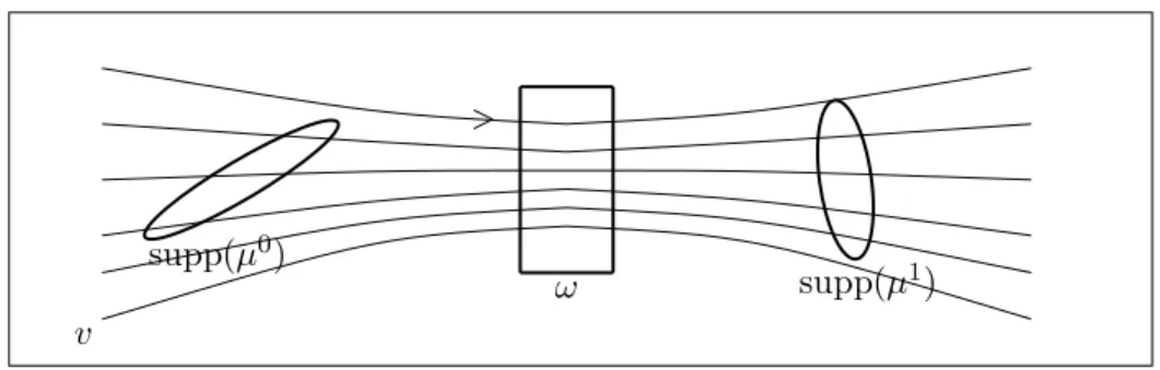
definition of the notion of approximate controllability in terms of Wasserstein distance. The main results of this article show that approximate and exact controllability de-pend on two main aspects: first, from a geometric point of view, the uncontrolled vector field v needs to send the support of µ0 to ω forward in time and the support of µ1 to ω
backward in time. This idea is formulated in the following condition:
Condition 1.1 (Geometric Condition). Let µ0, µ1 be two probability measures on Rd
satisfying:
(i) For each x0 P supppµ0q, there exists t0 ą 0 such that Φv
t0px0q P ω, where Φvt is the
flow associated to v, i.e. the solution to the Cauchy problem
#
9xptq “ vpxptqq for a.e. t ą 0, xp0q “ x0.
(ii) For each x1 P supppµ1q, there exists t1ą 0 such that Φv
´t1px1q P ω.
This geometric aspect is illustrated in Figure 1.
supppµ0q
ω supppµ1q
v
Figure 1: Geometric Condition 1.1.
Remark 1. Condition 1.1 is the minimal one that we can expect to steer any initial condition to any target. Indeed, if there exists a point x0 of the interior of supppµ0q for
which the first item of the Geometrical Condition 1.1 is not satisfied, then there exists a part of the population of the measure µ0 that never intersects the control region, thus
The second aspect that we want to highlight is the following: The measures µ0 and
µ1 need to be sufficiently regular with respect to the flow generated by v` 1
ωu. Three
cases are particularly relevant:
a) Controllability with Lipschitz controls
If we impose the classical Carath´eodory condition of 1ωu being Lipschitz in space,
measurable in time and uniformly bounded, then the flow Φvt`1ωu is an homeomorphism (see [10, Th. 2.1.1]). As a result, one can expect approximate controllability only, since for general measures there exists no homeomorphism sending one to another. For more details, see Section 4.1. We then have the following result:
Theorem 1.1 (Main result - Controllability with Lipschitz control). Let µ0, µ1 be two
probability measures on Rdcompactly supported, absolutely continuous with respect to the
Lebesgue measure and satisfying Condition 1.1. Then there exists T such that System (1) is approximately controllable on the time interval r0, T s from µ0 to µ1 with a control
1ωu: Rdˆ R`Ñ Rd uniformly bounded, Lipschitz in space and measurable in time.
We give a proof of Theorem 1.1 in Section 3. This proof is a constructive one and strongly uses the fact that the velocity vector field v is autonomous, i.e. not dependent on time. Moreover, it is clear that the extension of our work to time dependent velocity vector fields should require a non-trivial modification of the Geometric Condition 1.1. For the initial measure µ0 (forward trajectory) the modification is simply the replacement
of the flow of the autonomous vector field with the flow of the non-autonomous one, starting from t“ 0. Instead, for the final measure µ1 (backward trajectories) one needs
to consider the non-autonomous vector field starting from the final time T , which is an unknown of the problem.
Remark2. Due to the finite speed of propagation outside of ω, approximate controllability cannot hold at arbitrary small time. The study of this minimal controllability time is carried on in the forthcoming paper [25].
Remark 3. If one removes the assumption of boundedness of v, replacing it with other conditions ensuring boundedness of the flow for each time (e.g. by imposing sub-linear growth), then the results presented here still hold. Indeed, it is sufficient to observe that we mainly deal with properties of the flow, that are preserved in this case.
If one instead removes the assumption of boundedness of the supports of µ0, µ1keeping
boundedness of v, it is clear that controllability does not hold in general. Indeed, one needs an infinite time to steer the whole mass of µ0 to the mass of µ1.
Finally, if one removes both boundedness of the supports and boundedness of the velocity v, it is possible to find examples of approximate controllability in finite time. For example, in R`with ω“ R`, consider the vector field vpxq “ x2, for which the flow is
Φv
tpx0q “ 1´tx0x0 , defined only for tă x´10 . Thus, one can verify that µ 0
“ 1r0,1s is sent to
µ1 “ 1
px`1q21r0,`8q at time T “ 1. Nevertheless, the problem under such less restrictive
hypotheses seems harder to study in its generality, even though adaptations of the method presented here seem possible. Moreover, our applications to crowd modeling and control always assume finite speed of propagation and measures with bounded support.
b) Controllability with vector fields inducing maximal regular flows To hope to obtain exact controllability of System (1) at least for absolutely continuous measures, it is then necessary to search among controls 1ωu with less regularity. A
(1) has been recently introduced by Ambrosio-Colombo-Figalli in [5], extending previous results by Ambrosio [3] and DiPerna-Lions [24]. Examples of vector fields satisfying such condition are Sobolev vector fields [24], and BV (bounded variation) vector fields with locally integrable divergence [3]. Thus, if we choose the admissible controls satisfying the setting of [5], it is not necessary that there exists an homeomorphism between µ0 and µ1.
For all such theories, given a vector field w, a suitable concept of flow Φw
t is introduced,
such as the maximal regular flow [5], generalizing the regular Lagrangian flow of [3]. Even though such flow does not enjoy all the properties of flows of Lipschitz vector fields, a common requirement is that the Lebesgue measure L restricted to an open bounded set Ais transported to a measure bounded from above by a multiple of the Lebesgue measure itself. In other terms, there exists of a constant Cą 0 such that for all t P r0, T s it holds
Φwt #L|Aď CL (2)
We will show in Section 4.1 that this condition implies the non-existence of controls exactly steering one absolutely continuous measure to another, for specific choices of µ0, µ1. Thus, even this setting does not allow to yield exact controllability.
It is also interesting to observe that Property (2) is often required as a necessary condition for a reasonable generalization of the standard theory of Ordinary Differential Equations. Indeed, for Lipschitz vector fields w, the constant C is given by eLippwqt. Then, in DiPerna-Lions such condition is required in [24, Eq. (7)] on both sides, while in Ambrosio it is required in [3, Eq (6.1)]. In this sense, the non-exact controllability seems a drawback of a desired condition for an even very general theory of Ordinary Differential Equations, rather than a goal to be reached.
c) Controllability with L2 controls
We then consider an even larger class of controls, that are general Borel vector fields. In this setting, we have exact controllability under the Geometric Condition 1.1 for any pairs of measures, even not absolutely continuous. Moreover, we prove that one can restrict the set of admissible controls to those that are L2 with respect to the measure
itself, i.e. to controls satisfying ż1
0
ż
Rd
|uptq|2dµptqdt ă 8. (3)
The main drawback is that, in this less regular setting, System (1) is not necessarily well-posed. In particular, one has not necessarily uniqueness of the solution. For this reason, one needs to describe solutions to System (1) as pairs p1ωu, µq, where µ is one
among the admissible solutions with control 1ωu.
Theorem 1.2 (Main result - Controllability with L2control). Let µ0, µ1 be two
probabil-ity measures on Rd compactly supported and satisfying Condition 1.1. Then, there exists
T ą 0 such that System (1) is exactly controllable on the time interval r0, T s from µ0
to µ1 in the following sense: there exists a couple
p1ωu, µq composed of a L2 vector field
1ωu : Rdˆ R` Ñ Rd and a time-evolving measure µ being weak solution to System (1)
(see Definition 3) and satisfying
µpT q “ µ1.
A proof of Theorem 1.2 is given in Section 4.
If µ0, µ1 satisfy the Geometric Condition 1.1, then
µ0, µ1 absolutely continuous
• approx. controllability with Lipschitz con-trol
• NO exact controllability with control in-ducing maximal regular flows
µ0, µ1
general measures
exact controllability with L2 control
This paper is organised as follows. In Section 2, we recall basic properties of the Wasserstein distance and the continuity equation. Section 3 is devoted to the proof of Theorem 1.1, i.e. the approximate controllability of System (1) with a Lipschitz localized vector field. Finally, in Section 4, we first show that exact controllability does not hold for Lipschitz controls or even vector fields inducing a maximal regular flow; we also prove Theorem 1.2, i.e. exact controllability of System (1) with a L2 localized vector field.
2
The Wasserstein distance and the continuity equation
In this section, we recall the definition and some properties of the Wasserstein distance and the continuity equation, which will be used all along this paper. We denote by PcpRdq
the space of probability measures in Rdwith compact support and for µ, ν P P
cpRdq. We
also introduce the classical partial ordering of measures: µď ν if A being ν-measurable implies A being µ-measurable and µpAq ď νpAq.
We denote by Πpµ, νq the set of transference plans from µ to ν, i.e. the probability measures on Rdˆ Rdsatisfying ż Rd dπpx, ¨q “ dµpxq and ż Rd dπp¨, yq “ dνpyq.
Definition 1. Let pP r1, 8q and µ, ν P PcpRdq. Define
Wppµ, νq “ inf πPΠpµ,νq $ ’ ’ & ’ ’ % ¨ ˚ ˝ ij RdˆRd |x ´ y|pdπ ˛ ‹ ‚ 1{p,/ / . / / -. (4)
The quantity is called the Wasserstein distance.
This is the idea of optimal transportation, consisting in finding the optimal way to transport mass from a given measure to another. For a thorough introduction, see e.g. [41].
We denote by Γ the set of Borel maps γ : RdÑ Rd. We now recall the definition of
Definition 2. For a γ P Γ, we define the push-forward γ#µ of a measure µ of Rd as
follows:
pγ#µqpEq :“ µpγ´1pEqq, for every subset E such that γ´1pEq is µ-measurable.
We denote by “AC measures” the measures which are absolutely continuous with respect to the Lebesgue measure and by Pac
c pRdq the subset of PcpRdq of AC measures.
On Pac
c pRdq, the Wasserstein distance can be reformulated as follows:
Property 2.1 (see [41, Chap. 7]). Let pP r1, 8q and µ, ν P Pac
c pRdq. It holds Wppµ, νq “ inf γPΓ #ˆż Rd |γpxq ´ x|pdµ ˙1{p : γ#µ“ ν + . (5)
The Wasserstein distance satisfies some useful properties: Property 2.2 (see [41, Chap. 7]). Let pP r1, 8q.
(i) The Wasserstein distance Wp is a distance on PcpRdq.
(ii) The topology induced by the Wasserstein distance Wp on PcpRdq coincides with the
weak topology. (iii) For all µ, νP Pac
c pRdq, the infimum in (5) is achieved by at least one minimizer.
The Wasserstein distance can be extended to all pairs of measures µ, ν compactly supported with the same total mass µpRdq “ νpRdq ‰ 0, by the formula
Wppµ, νq “ µpRdq1{pWp ˆ µ µpRdq, ν νpRdq ˙ .
In the rest of the paper, the following properties of the Wasserstein distance will be also helpful:
Property2.3 (see [37, 41]). Let µ, ρ, ν, η be four positive measures compactly supported
satisfying µpRdq “ νpRdq and ρpRdq “ ηpRdq.
(i) For each pP r1, 8q, it holds
Wpppµ ` ρ, ν ` ηq ď Wpppµ, νq ` Wpppρ, ηq. (6)
(ii) For each p1, p2P r1, 8q with p1 ď p2, it holds
#
Wp1pµ, νq ď Wp2pµ, νq,
Wp2pµ, νq ď diampXq1´p1{p2Wp1p1{p2pµ, νq,
(7)
where X contains the supports of µ and ν.
We now recall the definition of the continuity equation and the associated notion of weak solutions:
Definition 3. Let T ą 0 and µ0be a measure in Rd. We said that a pairpµ, wq composed
with a measure µ in Rdˆ r0, T s and a vector field w : Rdˆ R`Ñ Rdsatisfying
żT
0
ż
Rd
|wptq| dµptqdt ă 8
is a weak solution to the system, called the continuity equation, #
Btµ` ∇ ¨ pwµq “ 0 in Rdˆ r0, T s,
µp0q “ µ0 in Rd, (8)
if for every continuous bounded function ξ : Rd Ñ R, the function t ÞÑ ş
Rdξ dµptq is
absolutely continuous with respect to t and for all ψP Cc8pRdq, it holds
d dt ż Rd ψ dµptq “ ż Rdx∇ψ, wptqy dµptq
for a.e. t and µp0q “ µ0.
Note that t ÞÑ µptq is continuous for the weak convergence, it then make sense to impose the initial condition µp0q “ µ0 pointwisely in time. Before stating a result of
existence and uniqueness of solutions for the continuity equation, we first recall the definition of the flow associated to a vector field.
Definition 4. Let w : RdˆR`Ñ Rdbe a vector field being uniformly bounded, Lipschitz
in space and measurable in time. We define the flow associated to the vector field w as the application px0, tq ÞÑ Φw
t px0q such that, for all x0 P Rd, tÞÑ Φwtpx0q is the solution to
the Cauchy problem #
9xptq “ wpxptq, tq for a.e. t ě 0, xp0q “ x0.
The following property of the flow will be useful all along the present paper:
Property 2.4 (see [37]). Let µ, ν P PcpRdq and w : Rdˆ R Ñ Rd be a vector field
uniformly bounded, Lipschitz in space and measurable in time with a Lipschitz constant equal to L. For each tP R and p P r1, 8q, it holds
WppΦwt#µ, Φwt #νq ď e pp`1q
p L|t|W
ppµ, νq. (9)
Similarly, let µ P Pac
c pRdq and w1, w2 : Rdˆ R Ñ Rd be two vector fields uniformly
bounded, Lipschitz in space with a Lipschitz constant equal to L and measurable in time. Then, for each tP R and p P r1, `8q, it holds
WppΦw1t #µ, Φw2t #µq ď eL|t|{p
eL|t|´ 1
L }w1´ w2}C0. (10) We now recall a standard result for the continuity equation:
Theorem 2.1 (see [41, Th. 5.34]). Let T ą 0, µ0 P P
cpRdq and w a vector field
uniformly bounded, Lipschitz in space and measurable in time. Then, System (8) admits a unique solution µ in C0pr0, T s; P
cpRdqq, where PcpRdq is equipped with the weak topology.
Moreover: (i) If µ0P Pac
c pRdq, then the solution µ to (8) belongs to C0pr0, T s; PcacpRdqq.
(ii) We have µptq “ Φw
We now recall the precise notions of approximate controllability and exact controlla-bility for System (1):
Definition 5. We say that:
‚ System (1) is approximately controllable from µ0 to µ1 on the time interval
r0, T s if for each ε ą 0 there exists a control 1ωu such that the corresponding
solutions µ to System (1) satisfies
Wppµ1, µpT qq ď ε. (11)
‚ System (1) is exactly controllable from µ0 to µ1 on the time interval r0, T s if
there exists a control 1ωu such that the corresponding solution to System (1) is
equal to µ1 at time T .
It is interesting to remark that, by using properties (7) of the Wasserstein distance, estimate (11) can be replaced by:
W1pµ1, µpT qq ď ε.
Thus, in this work, we study approximate controllability by considering the distance W1
only.
Remark 4. One can be interested in proving approximate controllability for a smaller set of controls, for example of class Ck in the space variable with some k ě 1. Due to the
estimate (10), the result of Theorem 1.1 still holds in this case, by density of Ckfunctions
in the space of Lipschitz function with respect to the C0 norm. Higher regularity in the
time variable can be achieved too with the same techniques.
A careful inspection of our proof shows that controls ensuring approximate control-lability are not only measurable in time, but they have a finite number of discontinuities in time, that can be smoothened in a small interval of size τ . The introduced error can be arbitrarily small, by using the fact that limτÑ0eLτ{ppeLτ ´ 1q “ 0.
3
Approximate controllability with a localized Lipschitz
control
In this section, we study approximate controllability of System (1) with localized Lip-schitz controls. More precisely, in Sections 3.1, we consider the case where the open connected control subset ω contains the support of both µ0 and µ1. We then prove
Theorem 1.1 in Section 3.2.
3.1 Approximate controllability with a Lipschitz control
In this section, we prove approximate controllability of System (1) with a Lipschitz control, when the open connected control subset ω contains the support of both µ0 and
µ1. Without loss of generality, we can assume that the vector field v is identically zero
by replacing u with u´ v in the control set ω.
We then study approximate controllability of system #
Btµ` divpuµq “ 0 in Rdˆ R`,
Proposition 3.1. Let µ0, µ1 P Pac
c pRdq compactly supported in ω. Then, for all T ą 0,
System (12) is approximately controllable on the time interval r0, T s from µ0 to µ1 with
a control u : Rdˆ R` Ñ Rd uniformly bounded, Lipschitz in space and measurable in time. Moreover, the solution µ to System (12) satisfies
supppµptqq Ă ω,
for all tP r0, T s.
Proof of Proposition 3.1. We assume that d :“ 2, but the reader will see that the proof can be clearly adapted to dimension one or to any other space dimension. In view to simplify the computations, we suppose that T :“ 1 and supppµiq Ă p0, 1q2 ĂĂ ω for
i“ 1, 2.
We first partition p0, 1q2. Let nP N˚, consider a
0 :“ 0, b0 :“ 0 and define the points
ai, bi for all iP t1, ..., nu by induction as follows: suppose that for a given i P t0, ..., n ´ 1u
the points ai and bi are defined, then the points ai`1 and bi`1 are the smallest values
such that ż pai,ai`1qˆR dµ0 “ 1 n and ż pbi,bi`1qˆR dµ1 “ 1 n.
Again, for each iP t0, ..., n ´ 1u, we consider ai,0 :“ 0, bi,0 :“ 0 and supposing that for
a given j P t0, ..., n ´ 1u the points ai,j and bi,j are already defined, ai,j`1 and bi,j`1 are
the smallest values such that ż Aij dµ0 “ 1 n2 and ż Bij dµ1 “ 1 n2,
where Aij :“ pai, ai`1q ˆ paij, aipj`1qq and Bij :“ pbi, bi`1q ˆ pbij, bipj`1qq. Since µ0 and
µ1 have a mass equal to 1 and are supported inp0, 1q2, then a
n, bnď 1 and ai,n, bi,nď 1
for all iP t0, ..., n ´ 1u. We give in Figure 2 an example of such partition. x2 x1 a0 a1 a01 a02 .. . ... a0pn´2q a0pn´1q a0n a2 a11 a12 .. . a1pn´2q a1pn´1q 1 n ¨ ¨ ¨ ¨ ¨ ¨ ai ai1 .. . aij aipj`1q .. . 1{n2 aipn´1q ai`1 ¨ ¨ ¨ ¨ ¨ ¨ an´2 apn´2q1 apn´2q2 .. . apn´2qpn´2q apn´2qpn´1q an´1 apn´1q1 apn´1q2 .. . apn´1qpn´2q apn´1qpn´1q an
Figure 2: Example of a partition for µ0.
If one aims to define a vector field sending each Aij to Bij, then some shear stress
define sets rAij ĂĂ Aij and rBij ĂĂ Bij for all i, j P t0, ..., n ´ 1u. We then send the mass
of µ0 from each rA
ij to rBij, while we do not control the mass contained in Aijz rAij. More
precisely, for all i, j P t0, ..., n ´ 1u, we define, as in Figure 3, a´i , a`i , a´ij, a`ij the smallest
values such that ż
pai,a´i qˆpaij,aipj`1qq
dµ0 “ ż pa`i,ai`1qˆpaij,aipj`1qq dµ0 “ 1 n3 and ż pa´i ,a`iqˆpaij,a´ijq dµ0 “ ż pa´i,a`iqˆpa`ij,aipj`1qq dµ0“ 1 nˆ ˆ 1 n2 ´ 2 n3 ˙ .
We similarly define b`i , b´i , b`ij, b´ij and finally define
1 nˆ ` 1 n2 ´ 2 n3 ˘ 1 n3 ai a´i a`i ai`1 aij a´ij a`ij aipj`1q r Aij
Figure 3: Example of cell.
r
Aij :“ pa´i , a`i q ˆ pa´ij, a`ijq and rBij :“ pb´i , b`i q ˆ pb´ij, b`ijq.
The goal is to build a solution to System (12) such that the corresponding flow Φu t
satisfies
ΦuTp rAijq “ rBij, (13)
for all i, jP t0, ..., n ´ 1u. We observe that we do not take into account the displacement of the mass contained in Aijz rAij. We will show that the mass of the corresponding term
tends to zero when n goes to infinity. The rest of the proof is divided into two steps. In a first step, we build a flow satisfying (13), then the corresponding vector field. In a second step, we compute the Wasserstein distance between µ1 and µpT q, showing that it
converges to zero when n goes to infinity. Step 1: We first build a flow satisfying (13). We recall that T :“ 1. For each i P t0, ..., n ´ 1u, we denote by c´i and c`i the linear functions equal to a´i and a`i at time t “ 0 and equal to b´i and b`i at time t“ T “ 1,
respectively, i.e. the functions defined for all tP r0, T s by:
c´i ptq “ pb´i ´ a´i qt ` a´i and c`i ptq “ pb`i ´ a`i qt ` a`i .
Similarly, for all i, j P t0, ..., n ´ 1u, we denote by c´ij and c`ij the linear functions equal
to a´ij and a`ij at time t“ 0 and equal to b´ij and b`ij at time t“ T “ 1, respectively, i.e. the functions defined for all tP r0, T s by:
c´ijptq “ pb´ij ´ a´ijqt ` a´ij and c`ijptq “ pb`ij ´ a`ijqt ` a`ij.
Consider the application being the following linear combination of c´i , c`i and c´ij, c`ij on r Aij, i.e. xpx0, tq :“ ˆ x1px0, tq x2px0, tq ˙ “ ¨ ˚ ˚ ˚ ˝ a`i ´ x0 1 a`i ´ a´i c´i ptq ` x 0 1´ a´i a`i ´ a´i c`i ptq a`ij ´ x0 2 a`ij ´ a´ij c´ijptq ` x 0 2´ a´ij a`ij´ a´ij c`ijptq ˛ ‹ ‹ ‹ ‚, (14)
where x0 “ px0 1, x
0
2q P rAij. Let us prove that an extension of the application px 0, tq ÞÑ
xpx0, tq is a flow associated to a vector field u. After some computations, we obtain
$ ’ & ’ % dx1 dt px 0, tq “ α iptqx1px0, tq ` βiptq @t P r0, T s, dx2 dt px 0, tq “ α ijptqx2px0, tq ` βijptq @t P r0, T s,
where for all tP r0, T s, $ ’ ’ ’ & ’ ’ ’ % αiptq “ b`i ´ b´i ` a´i ´ a`i c`i ptq ´ c´i ptq , βiptq “ a`i b´i ´ a´i b`i c`i ptq ´ c´i ptq, αijptq “ b`ij ´ b´ij ` a´ij´ a`ij c`ijptq ´ c´ijptq , βijptq “ a`ijb´ij ´ a´ijb`ij c`ijptq ´ c´ijptq.
The last quantities are well defined since for all i, j P t0, ..., n ´ 1u and t P r0, T s "
|c`i ptq ´ c´i ptq| ě maxt|a`i ´ a´i |, |b`i ´ b´i |u,
|c`ijptq ´ c´ijptq| ě maxt|a`ij ´ a´ij|, |b`ij ´ b´ij|u. For all tP r0, T s, consider the set
r
Cijptq :“ pc´i ptq, c`i ptqq ˆ pc´ijptq, c`ijptqq.
We remark that rCijp0q “ rAij and rCijpT q “ rBij. On
r
Cij :“ tpx, tq : t P r0, T s, x P rCijptqu,
we then define the vector field u by "
u1px, tq “ αiptqx1` βiptq,
u2px, tq “ αijptqx2` βijptq,
for all px, tq P rCij (x “ px1, x2q). Notice that the sets rCij do not intersect. Thus, we
extend u by a uniform bounded C8function outsideYijCrij, then u is a C8 function and
it satisfies supppuq Ă ω.
Then, System (1) admits an unique solution and the flow on rCij is given by (14).
Step 2: We now prove that the refinement of the grid provides convergence to the target µ1, i.e. W1pµ1, µpT qq ÝÑ nÑ80. We remark that ż r Bij dµpT q “ ż r Bij dµ1“ 1 n2 ´ 2 n3 ´ 2 n ˆ 1 n2 ´ 2 n3 ˙ “ pn ´ 2q 2 n4 . Hence, by defining R:“ p0, 1q2 z ď ij r Bij, we also have ż R dµpT q “ ż R dµ1“ 1 ´ pn ´ 2q 2 n2 .
Using (6), it holds W1pµ1, µpT qq ď n ř i,j“1 W1pµ1 | rBij, µpT q| rBijq ` W1pµ 1 |R, µpT q|Rq. (15)
We now estimate each term in the right-hand side of (15). Since we deal with AC measures, using Properties 2.2,
there exist measurable maps γij : R2 Ñ R2, for all i, j P t0, ..., n´1u, and γ : R2Ñ R2
such that $ ’ ’ ’ ’ & ’ ’ ’ ’ % γij#pµ1| rBijq “ µpT q| rBij, W1pµ1 | rBij, µpT q| rBijq “ ż r Bij |x ´ γijpxq|dµ1pxq and $ ’ ’ ’ & ’ ’ ’ % γ#pµ1 |Rq “ µpT q|R, W1pµ1|R, µpT q|Rq “ ż R |x ´ γpxq|dµ1pxq.
In the first term in the right hand side of (15), observe that γij moves masses inside rBij
only. Thus, for all i, j P t0, ..., n ´ 1u, using the triangle inequality,
W1pµ1 | rBij, µpT q| rBijq “ ż r Bij |x ´ γijpxq|dµ1pxq ď rpb`i ´ b´i q ` pb`ij ´ b´ijqs ż r Bij dµ1pxq ď pb`i ´ b´i ` b`ij´ b´ijq pn ´ 2q2 n4 . (16)
For the second term in the right-hand side of (15), observe that γ moves a small mass in the bounded setp0, 1q. Thus it holds
W1pµ1|R, µpT q|Rq “ ż R |x ´ γpxq|dµ1pxq ď 2 ˆ 1´pn ´ 2q 2 n2 ˙ “ 8n´ 1 n2 . (17)
Combining (15), (16) and (17), we obtain
W1pµ1, µpT qq ď ˜ n ř i,j“1 pb`i ´ b´i ` b`ij´ b´ijq pn ´ 2q2 n4 ¸ ` 8n´ 1 n2 ď 2npn ´ 2q 2 n4 ` 8 n´ 1 n2 nÑ8ÝÑ 0.
Remark 5. It is not possible in general to build a Lipschitz vector field sending directly each Aij to Bij using the strategy developed in the proof of Proposition 3.1. Indeed, we
would obtain discontinuous velocities on the lines ci. Figure 4 illustrates this phenomenon
in the case n“ 2.
3.2 Approximate controllability with a localized regular control
This section is devoted to prove Theorem 1.1: we aim to prove approximate controlla-bility of System (1) with a Lipschitz localized control. This means that we remove the constraints supppµ0q Ă ω, supppµ1q Ă ω and v :“ 0, that we used in Section 3.1. On the
other side, we impose Condition 1.1. Before the main proof, we need three useful results. First of all, we give a consequence of Condition 1.1:
a0 a1 a2 a00“ a10 a11 a01 a02“ a12 b0 b1 b2 b00“ b10 b11 b01 b02“ b12
Figure 4: Shear stress (left: µ0, right: µ1)
Condition 3.1. There exist two real numbers T˚
0, T1˚ ą 0 and a nonempty open set
ω0 ĂĂ ω such that
(i) For each x0 P supppµ0q, there exists t0 P r0, T˚
0s such that Φvt0px0q P ω0,where Φvt
is the flow associated to v.
(ii) For each x1 P supppµ1q, there exists t1P r0, T˚
1s such that Φv´t1px1q P ω0.
Lemma 3.1. If Condition 1.1 is satisfied for µ0, µ1 P P
cpRdq, then Condition 3.1 is
satisfied too.
Proof. We use a compactness argument. Let µ0 P P
cpRdq and assume that Condition
1.1 holds. Let x0 P supppµ0q. Using Condition 1.1, there exists t0px0q ą 0 such that
Φvt0 px0
qpx
0q P ω. Choose rpx0q ą 0 such that B
rpx0qpΦv t0 px0 qpx 0qq ĂĂ ω, where B rpx0q
denotes the open ball of radius rą 0 centered at point x0 in Rd. Such rpx0q exists, since
ω is open. By continuity of the application x1 ÞÑ Φv t0
px0 qpx
1q (see [10, Th. 2.1.1]), there
exists ˆrpx0q such that
x1P Bˆrpx0qpx0q ñ Φv t0 px0 qpx 1q P B rpx0qpΦv t0 px0 qpx 0qq.
Since µ0 is compactly supported, we can find a set tx0
1, ..., x0N0u Ă supppµ0q such that
supppµ0q Ă N0 ď i“1 Brpxˆ 0 iqpx 0 iq.
We similarly build a settx1
1, ..., x1N1u Ă supppµ1q. Thus Condition 3.1 is satisfied for
Tk˚ :“ maxttkpxkiq : i P t1, ..., Nkuu, with k“ 0, 1 and ω0 :“ ˜N0 ď i“1 Brpx0 iqpΦ v t0px0 iqpx 0 iqq ¸ ď˜ďN1 i“1 Brpx1 iqpΦ v ´t1px1 iqpx 1 iqq ¸ ĂĂ ω.
The second useful result is the following proposition, showing that we can store a large part of the mass of µ0 in ω, under Condition 3.1.
Proposition 3.2. Let µ0 P Pac
c pRdq satisfying the first item of Condition 3.1. Then, for
all εą 0, there exists a space-dependent vector field 1ωuLipschitz and uniformly bounded
and a Borel set AĂ Rd such that
µ0pAq “ ε and supppΦvT`1ωu˚ 0
#µ0|Acq Ă ω. (18)
Proof. For each kP N˚, we denote by ωk the closed set defined by
ωk:“ tx0 P Rd: dpx0, ωc0q ě 1{ku
and a cutoff function θkP C8pRdq satisfying
$ & % 0ď θk ď 1, θk “ 1 in ωc0, θk “ 0 in ωk.
For all x0 P supppµ0q, we define
t0px0q :“ inftt P R`: Φvtpx 0
q P ω0u and tkpx0q :“ inftt P R `
: Φvtpx0q P ωku.
For all kP N˚, we consider
uk:“ pθk´ 1qv (19)
and
Sk:“ tx0 P supppµ0qzω0 :Ds P pt0px0q, tkpx0qq, s.t. Φvspx0q P ωc0u.
The rest of the proof is divided into three steps:
• In Step 1, we prove that the range of the flow associated to x0with the control ukis included in the range of the flow associated to x0without control, i.e. tΦv`uk
t px0q :
tě 0u Ă tΦv
tpx0q : t ě 0u.
• In Step 2, we show that Sk is a Borel set for all kP N˚. • In Step 3, we prove that for a K large enough we have
µ0pωzωKq ` µ0pSKq ď ε. (20)
Step 1: Consider the flow yptq :“ Φv
tpx0q associated to x0 without control, i.e. the
solution to #
9yptq “ vpyptqq, t ě 0, yp0q “ x0
and the flow zkptq :“ Φv`ukt px0q associated to x0 with the control uk given in (19), i.e.
the solution to #
9zkptq “ pv ` ukqpzkptqq “ θkpzkptqq ˆ vpzkptqq, t ě 0,
zkp0q “ x0.
(21)
We use the time change γk defined as the solution to the following system
# 9
γkptq “ θkpypγkptqqq, t ě 0,
γkp0q “ 0.
Since θk and y are Lipschitz, then System (22) admits a solution defined for all times.
We remark that ξk:“ y ˝ γk is solution to System (21). Indeed, for all tě 0 it holds
#
9ξkptq “ 9γkptq ˆ 9ypγkptqq “ θkpξkptqq ˆ vpξkptqq, t ě 0,
ξkp0q “ ypγkp0qq “ yp0q.
By uniqueness of the solution to System (21), we obtain ypγkptqq “ zkptq for all t ě 0.
Using the fact that 0ď θ ď 1 and the definition of γk, we have
$ & % γk increasing, γkptq ď t @t P r0, tkpx0qs, γkptq ď tkpx0q @t ě tkpx0q.
We deduce that, for all x0P supppµ0q, it holds
tzkptq : t ě 0u Ă typsq : s P r0, tkpx0qsu.
Step 2: We now prove that Sk is a Borel set by showing that the set
Rk:“ tx0 P Rd: t0px0q ă 8 and Ds P pt0px0q, tkpx0qq s.t. Φvspx 0
q P ωc0u
is open. Let kP N˚, x0 be an element of R
k and search rpx0q ą 0 such that Brpx0qpx0q Ă
Rk.
There exists sP pt0px0q, tkpx0qq such that Φsvpx0q P ωc0. Since ωc0 is open, for a βą 0,
we have BβpΦvspx0qq Ă ωc0. By continuity of the application x
1 ÞÑ Φv spx1q, there exists rpx0q ą 0 such that x1P Brpx0 qpx0q ñ Φvspx 1 q P BβpΦvspx 0 qq.
Thus, for all kP N˚, Rk is open. As Sk “ RkX supppµ0q X ωc0, Sk is a Borel set.
Step 3: We now prove that (20) holds for a K large enough. Since we deal with we AC measure, there exists K0 P N˚ such that for all kě K0
µ0pω0zωkq ď ε{2.
Argue now by contradiction to prove that there exists K1 ě K0 such that
µ0pSK1q ď ε{2.
Assume that µ0pS
kq ą ε{2 for all k ě K0. Using the inclusion Sk`1 Ă Sk, we deduce
that µ0 ˜ č kPN˚ Sk ¸ ě ε{2.
Since µ0 is absolute continuous with respect to λ (the Lebesgue measure), there exists
αą 0 such that λ ˜ č kPN˚ Sk ¸ ě α.
We deduce that the intersection of the set Sk is nonempty. Let x0 P supppµ0qzω0 be an
element of this intersection. By definition of Sk, for all kě K0, there exists sk satisfying
"
skP pt0px0q, tkpx0qq,
Φv
skpx0q P ωc0.
Moreover, the convergence of tkpx0q to t0px0q, implies that
sk Ñ t0px0q. (24)
Using the continuity of x1 ÞÑ Φv
tpx1q and the definition of t0px0q, there exists β ą 0 such
that
Φvtpx0q P ω
0 for all tP pt0, t0` βq. (25)
We deduce that (25) contradicts (23) and (24). Thus there exists KP N˚ such that
µ0pSKq ` µ0pωzωKq ď ε.
Since we deal with AC measures, we add a Borel set to have the equality in (18), i.e. there exists a Borel set S such that
µ0pSKY ωzωKY Sq “ ε.
We conclude that, for u defined by uptq :“ u1 :“ u
K for all tP r0, T0˚s,
and A :“ SKY ωzωKY S, Properties (18) are satisfied.
The third useful result for the proof of Theorem 1.1 allows to approximately steer a measure contained in ω to a measure contained in an open hypercube SĂĂ ω.
Proposition 3.3. Let µ0 P Pac
c pRdq satisfying supppµ0q Ă ω. Define an open hypercube
S strictly included in ωz supppµ0q and choose δ ą 0. Then, for all ε ą 0, there exists a
vector field 1ωu, Lipschitz and uniformly bounded and a Borel set A such that
µ0pAq “ ε and supppΦvδ`1ωu#µ0
|Acq Ă S.
Proof. Consider S0 a nonempty open set of Rd of class C8 strictly included in S and rω
an open set of Rd of class C8 satisfying
supppµ0q Y S ĂĂ rωĂĂ ω.
An example is given in Figure 5. From [28, Lemma 1.1, Chap. 1] (see also [18, Lemma 2.68, Chap. 2]), there exists a function ηP C2
prωq satisfying
κ0 ď |∇η| ď κ1 in rωzS0, ηą 0 in rω and η“ 0 on Brω, (26)
with κ0, κ1 ą 0. Let k P N˚. Consider uk : RdÑ Rd Lipschitz and uniformly bounded
satisfying
uk :“
"
k∇η´ v in rω, 0 in ωc.
Let x0 P supppµ0q. Consider the flow z
kptq “ Φv`ukt px0q associated to x0 with the
control uk, i.e. the solution to system
#
9zkptq “ vpzkptqq ` ukpzkptqq, t ě 0,
zkp0q “ x0.
(27)
The different conditions in (26) imply that
ω r ω S S0 supppµ0q Figure 5: Construction of rω
where n represents the outward unit normal toBrω. Since supppµ0
q Ă rω, it holds zkptq P rω
for all tě 0, otherwise, by taking the scalar product of (27) and n on Brω, we obtain a contradiction with (28). We now prove that there exists Kpx0q P N˚such that for all kě
Kpx0q there exists t
kpx0q P p0, δq such that zkptkpx0qq belongs to S0. By contradiction,
assume that there exists a sequencestknunPN˚ Ă N˚ such that for all tP p0, δq
zknptq P S0c. (29)
Consider the function fn defined for all tP r0, δs by
fnptq :“ knηpzknptqq. (30)
Its time derivative is given for all tP r0, δs by 9
fnptq “ kn9zknptq ¨ ∇ηpzknptqq “ k2n|∇ηpzknptqq|2
Then, using (29), properties (26) of η and definition (30) of fn, it holds
fnpδq ě k2nκ20δ and fnpδq ď kn}η}8.
We observe that the two last inequalities are in contradiction for n large enough. Then there exists Kpx0q P N˚ such that for all kě Kpx0q there exists t
kpx0q P p0, δq such that
zkptkpx0qq belongs to S0. By continuity, there exists rpx0q ą 0 such that Φ
v`uKpx0 q tKpx0 qpx0
qpx 1q
belongs to S0 for all x1 P Brpx0
qpx0q. Since v ` uk is linear with respect to k in rω, then,
using the same argument as in Step 1 of the proof of Proposition 3.2, the range of the flow Φv`uk¨ is independent of k. Thus, for all kě Kpx0q there exists t0kpx0q P p0, δq such
that Φv`ukt0 kpx
0qpx 1q P S
0 for all x1 P Brpx0
qpx0q. By compactness, there exists tx01, ..., x0N0u
such that supppµ0q Ă N0 ď i“1 Brpx0 iqpx 0 iq.
We deduce that for K :“ maxitKpx0iqu, for all x0 P supppµ0q there exists t0px0q for
which Φv`uKt0px0qpx
0q belongs to S
0. We remark that the first item of Condition 3.1 holds
replacing ω, ω0 and T0˚ by S, S0 and δ, respectively. We conclude applying Proposition
Remark 6. An alternative method to prove Proposition 3.3 involves building an explicit flow composed with straight lines as in the proof of Proposition 3.1. However, for such method we need to assume that ω is convex, contrarily to the more general approach developed in the proof of Proposition 3.3.
We now have all the tools to prove Theorem 1.1.
Proof of Theorem 1.1. Consider µ0, µ1 satisfying Condition 1.1. By Lemma 3.1, there
exist T0˚, T1˚, ω0for which µ0, µ1satisfy Condition 3.1. Let δ, εą 0 and T :“ T0˚`T1˚`δ.
We now prove that we can construct a Lipschitz uniformly bounded and control 1ωusuch
that the corresponding solution µ to System (1) satisfies W1pµpT q, µ1q ď ε.
Denote by T0 :“ 0, T1 :“ T0˚, T2 :“ T0˚ ` δ{3, T3 :“ T0˚` 2δ{3, T4 :“ T0˚` δ and
T5 :“ T0˚` T1˚` δ. Also fix an open hypercube S ĂĂ ωzω0. There exists R ą 0 such
that the supports of µ0 and µ1 are strictly included in a hypercube with edges of length
R. Define
R:“ R ` T ˆ sup
Rd
|v|.
Applying Proposition 3.2 onrT0, T1s Y rT4, T5s and Proposition 3.3 on rT1, T2s Y rT3, T4s,
we can construct some space-dependent controls u1, u2, u4, u5 Lipschitz and uniformly
bounded, with supppuiq Ă ω, and two Borel sets A0 and A1 such that
µ0pA0q “ µ1pA1q “
ε 2dR, the solution forward in time to
$ ’ & ’ % Btρ0` ∇ ¨ ppv ` 1ωu1qρ0q “ 0 in Rdˆ rT0, T1s, Btρ0` ∇ ¨ ppv ` 1ωu2qρ0q “ 0 in Rdˆ rT1, T2s, ρ0pT0q “ µ0|Ac 0 in R d
and the solution backward in time to $ ’ & ’ % Btρ1` ∇ ¨ ppv ` 1ωu5qρ1q “ 0 in Rdˆ rT4, T5s, Btρ1` ∇ ¨ ppv ` 1ωu4qρ1q “ 0 in Rdˆ rT3, T4s, ρ1pT5q “ µ1|Ac 1 in R d
satisfy supppρ0pT2qq Ă S and supppρ1pT3qq Ă S. By conservation of the mass, we remark
that |ρ0pT2q| “ |ρ1pT3q| “ 1 ´ ε{2dR. We now apply Proposition 3.1 to approximately
steer ρ0pT2q to ρ1pT3q inside S as follows: we find a control u3 on the time intervalrT2, T3s
satisfying supppu3q Ă S such that the solution ρ to
# Btρ` ∇ ¨ ppv ` 1ωu3qρq “ 0 in Rdˆ rT2, T3s, ρpT2q “ ρ0pT2q in Rd satisfies W1pρpT3q, ρ1pT3qq ď ε 2e2LpT5´T3q,
where L is the uniform Lipschitz constant for u4 and u5. Thus, denoting by u the
concatenation of u1, u2, u3, u4, u5 on the time interval r0, T s, we approximately steer
µ0|Ac 0 to µ
1 |Ac
1, since by (9) the solution µ to
# Btµ` ∇ ¨ ppv ` 1ωuiqµq “ 0 in Rdˆ rTi´1, Tis, i P t1, ..., 5u, µp0q “ µ0 |Ac 0 in R d
satisfies W1pΦv`uT #µ0|Ac 0, µ 1 |Ac 0q “ W1pµpT5q, µ 1 |Ac 1q ď e 2LpT5´T3q ε 2e2LpT5´T3q “ ε 2. (31) Since we deal with AC measures, using Properties 2.2, there exists a measurable map γ : RdÑ Rd such that $ & % γ#µ1 |A1 “ Φ v`u T #µ 0 |A0,
W1pΦv`uT #µ0|A0, µ1|A1q “
ż
Rd
|x ´ γpxq|dµ1|A1pxq.
We deduce that
W1pΦv`uT #µ0|A0, µ1|A1q “
ż Rd|x ´ γpxq|dµ 1 |A1pxq ď dR ˆ ε 2dR “ ε 2. (32) Inequalities (6), (31) and (32) leads to the conclusion:
W1pΦv`uT #µ0, µ1q ď W1pΦv`uT #µ0|Ac 0, µ 1 |Ac 1q ` W1pΦ v`u T #µ 0 |A0, µ1|A1q ď ε.
4
Exact controllability
In this section, we study exact controllability for System (1). In Section 4.1, we show that exact controllability of System (1) does not hold for Lipschitz or controls inducing maximal regular flows. In Section 4.2, we prove Theorem 1.2, i.e. exact controllability of System (1) with a L2 localized control under some geometric conditions.
4.1 Negative results for exact controllability
In this section, we show that exact controllability does not hold in general for Lipschitz controls or even vector fields inducing a maximal regular flow. We will see that topological aspects play a crucial role at this level.
a) Non exact controllability with Lipschitz controls
As explained in the introduction, if we impose the classical Carath´eodory condition of 1ωu : Rdˆ R` Ñ Rd being uniformly bounded, Lipschitz in space and measurable in
time, then the flow Φvt`1ωu is a homeomorphism (see [10, Th. 2.1.1]). More precisely, the flow and its inverse are locally Lipschitz. This implies that the support of µ0 and
µpT q are homeomorphic. Thus, if the support of µ0 and µ1 are not homeomorphic, then
exact controllability does not hold with Lipschitz controls. In particular, we cannot steer a measure which support is connected to a measure which support is composed of two connected components with Lipschitz controls and conversely.
b) Non exact controllability with vector fields inducing maximal regular flows To hope to obtain exact controllability of System (1) at least for AC measures, it is then necessary to search for a control with less regularity. A weaker condition on the regularity of the vector field for the well-posedness of System (1) has been given in [5], generalizing previous conditions in [3, 24]. We first briefly recall the main definitions and results of such theory. We then prove that, in such setting, exact controllability between
some pairs of AC measures µ0, µ1 does not hold, even when the Geometric Condition 1.1
is satisfied.
We first recall the definition of maximal regular field in [5, Def. 4.4], and the cor-responding existence result [5, Thm. 5.7]. In our setting, we aim to find a flow that is defined on the whole space Rd for all timesr0, T s. Then, we present a simplified version
of maximal regular flows, with no hitting time or blow-up of trajectories. The notation is then simplified too.
Definition 6. Let w : Rdˆ p0, T q Ñ Rd be a Borel vector field. We say that a Borel
map Φw
t is a maximal regular flow relative to w if it satisfies:
1. for almost every xP Rd, the function Φw
tpxq is absolutely continuous with respect to
tand it solves the ordinary differential equation 9x “ wpt, xptqq with initial condition Φwtpxq “ x;
2. for any open bounded set AĂ Rd, there exists a compressibility constant CpAq such
that for all tP r0, T s, it holds
Φwt#L|Aď CpAqL. (33)
Theorem 4.1. Let w : Rdˆ p0, T q Ñ Rd be a Borel vector field satisfying the following
conditions:
a) şT0 şA|wpt, xq| dx dt ă 8 for any open bounded set A Ă Rd;
b) for any non-negative ¯ρ P L8`pRdq with compact support and any closed interval
ra, bs Ă p0, T q, the continuity equation
Btρt` ∇ ¨ pwρtq “ 0 in Rdˆ pa, bq
admits at most one weakly˚ continuous solution for tP ra, bs:
tÞÑ ρtP L8pra, bs; L8`pRdqq X tf s.t. supppf q compact subset of Rdˆ ra, bsu
with ρa“ ¯ρ.
c) for any open bounded set AĂ Rd it holds
divpwpt, .qq ě mptq in A, with LpAq :“ żT
0
|mptq| dt ă 8. (34)
Then, the maximal regular flow Φwt relative to w exists and is unique. Moreover, for any
open compact set A, the compressibility constant CpAq in (33) can be chosen as eLpAq.
For simplicity, we will study two examples of non-controllability in the 1-D setting only. It is then easy to observe that maximal regular flows preserve the order with respect to the initial data, as Lipschitz flows.
Proposition 4.1. Let w be a Borel vector field satisfying conditions of Theorem 4.1,
and Φw
t be the associated maximal regular flow. It then holds
Proof. Following the proof of [5, Thm. 5.2], build a family of mollified vector fields wε
for w: they are all Lipschitz, then they preserve the order xď y ñ Φwεt pxq ď Φwεt pyq for all x, y P R, as a classical property of Lipschitz vector fields in R. By letting wε á w
weakly in L1pp0, T q ˆ Aq for all A open bounded, and observing that other hypotheses of
the Stability Theorem 6.2 in [5] are satisfied, one has the result.
We are now ready to present two examples of pairs of AC measures µ0, µ1 in R for
which exact controllability does not hold with vector fields inducing maximal regular flows.
Exemple 4.1. For simplicity, we choose v” 0 and ω “ p´2, 2q from now on. For the first example, we define µ0 “ 1
r0,1sLand µ1pxq “ 12x ´1
21
p0,1qL. It is clear that the Geometric
Condition 1.1 is satisfied. Assume now that a Borel control u satisfying conditions of Theorem 4.1 steering µ0 to µ1 at a given time T ą 0 exists. Then, the associated
maximal regular flow both satisfies µ1 “ Φu
T#µ0 and there exists C “ Cpp0, 1qq such
that Φu
T#µ0 ď CL. Thus, we deduce that µ1 ď CL, which is in contradiction with the
definition of µ1.
Exemple 4.2. It is clear that the previous example is based on the fact that there exists measures that are absolutely continuous with respect to L and such that their Radon-Nikodym density are L1 functions that are not L8. One can then be interested in proving
exact controllability between measures of the form ρpxqL with ρpxq P L8pRq. Also in
this case, one has examples of non exact controllability. Indeed, consider again v ” 0 and ω “ p´2, 2q. Define ν0
pxq “ 2x1r0,1sL and ν1 “ 1r0,1sL. We prove now that also
in this case, there exists no control inducing maximal regular flows and realizing exact controllability. By contradiction, assume that such control w exists; thus, the associated flow Φu t satisfies ΦuT#ν 0 “ ν1. Then ż1 0 1ts : Φ u TpsqďΦuTpxqu2s ds“ ż1 0 1tsďΦ u Tpxquds,
Recall now that the flow preserves the ordering, then it necessarily holds żx 0 2s ds“ żΦu Tpxq 0 1 ds, i.e. Φu Tpxq “ x
2. If such a flow exists, then one can apply it to µ0 in the first example.
It then holds şx01 ds “ şΦuTpxq 0 1 2s ´1 2ds, i.e. Φu T#µ 0 “ µ1. Thus, Φu
T realizes the exact
control from µ0 to µ1. Contradiction. Then, there exist no control inducing maximal
regular flows and exactly steering ν0 to ν1.
Exemple 4.3. One can be interested in finding counterexamples to exact controllability in Rd with dą 1. The Example 4.1 for non exact controllability can be adapted to this
setting, by considering µ0“ LpB
1p0qq´11B1p0qLand µ1 “ ρ1pxqL with ρ1 being a L1 but
not L8 function. The counterexample in Example 4.2 can be adapted too, even though computations cannot be carried out easily by applying useful monotony properties.
4.2 Exact controllability with L2 controls
In this section, we prove Theorem 1.2, i.e. exact controllability of System (1) in the following sense: there exists a couplep1ωu, µq solution to System (1) satisfying µpT q “ µ1.
Before proving Theorem 1.2, we need three useful results. The first one is the following proposition, showing that we can store the whole mass of µ0 in ω, under Condition 3.1.
It is the analogue of Proposition 3.2. In this case, we control the whole mass, but we do not have necessarily uniqueness of the solution to System (1).
Proposition 4.2. Let µ0 P P
cpRdq satisfying the first item of Condition 3.1. Then
there exists a couple p1ωu, µq composed of a L2 vector field 1ωu : Rdˆ R` Ñ Rd and a
time-evolving measure µ being weak solution to System (1) and satisfying
supppµpT0˚qq Ă ω.
Proof. For each x0P Rd, we denote by
rt0px0q :“ inftt ě 0 : Φv
tpx0q P ω0u
and consider the application Ψ¨px0q defined for all t ě 0 by
Ψtpx0q “ # Φvtpx0q if tď rt0px0q, Φv rt0px0qpx 0q otherwise.
For all tě 0, the application Ψt is a Borel map. Consider µ defined for all tě 0 by
µptq :“ Ψt#µ0.
We remark that, for all t, sP r0, T˚
0s such that t ě s,
µptq “ Ψt´s#µpsq. (35)
Since Φv
¨px0q is Lipschitz, for all x0 P Rd and tP r0, T0˚s, it holds
|Ψtpx0q ´ x0| ď C mintt, t0px0qu ď Ct. (36)
Combining (35) and (36), we deduce for all t, sP r0, T0˚s with s ď t
W22pµpsq, µptqq ď ż Rd|Ψt´spxq ´ x| 2 dµpsq ď sup xPRd |Ψt´spxq ´ x|2 ď C|t ´ s|2.
We deduce that the metric derivative|µ1| of µ defined for all t P r0, T0˚s by
|µ1|ptq :“ lim
sÑt
W2pµptq, µpsqq
|t ´ s| (37)
is uniformly bounded onr0, T˚
0s. Then µ is an absolute continuous curve on PcpRdq (see
[4, Def. 1.1.1]). Using [4, Th. 8.3.1], there exists a Borel vector w : Rdˆ p0, T˚
0q Ñ Rd
satisfying
}wptq}L2
pµptq;Rdqď |µ1|ptq a.e. t P r0, T0˚s
and the couplepw, µq is a weak solution to #
Btµ` ∇ ¨ pwµq “ 0 in Rdˆ r0, T0˚s,
µp0q “ µ0 in Rd. (38)
By the uniform bound on the metric derivative, it holds that w is a L2 vector field.
Moreover, for all tP r0, T˚
0s, it holds
wptq P TanµptqpPcpRdqq :“ t∇ϕ : ϕ P Cc8pRdqu L2
(see [4, Def. 8.4.1]). Consider an open set ω1 of class C8 satisfying ω0 ĂĂ ω1 ĂĂ ω.
We now prove that wptq coincides with vptq in supppµptqqzω1 a.e. t P r0, T0˚s, i.e. we
can choose u “ 0 outside ω. Fix t P r0, T0˚s and consider x P supppµptqq X ωc1. There
necessarily exists x0 P supppµ0q such that Φv
tpx0q “ x, otherwise x P Bω0. Moreover for
a B :“ Brpx0q with r ą 0 ΦvspBq ĂĂ ω0c for all sP r0, ts, otherwise there exists s P r0, ts
for which Φv
spx0q P Bω0. Thus
Φvt “ Ψt in B. (39)
We denote by A :“ Φv
tpBq. We now prove that
Ψ´1t pAq “ pΦv
tq´1pAq. (40)
Consider x P pΦv
tq´1pAq. Equality (39) implies Φvtpxq “ Ψtpxq. Then x P Ψ´1t pAq.
Consider now x P Ψ´1t pAq, which means Ψtpxq P A. Using the fact that A X ω0 ‰ 0,
tă rx0pxq. Then Ψ
tpxq “ Φvtpxq and x P pΦvtq´1pAq. Thus (40) holds. By definition of
the push forward,
µ|Aptq “ Ψt#pµ0|Ψ´1
t pAqq and pΦ v
t#µ0q|A “ Φvt#pµ0|Φ´1 t pAqq.
Since Ψt“ Φvt on the set B“ pΦvtq´1pAq “ Ψ´1t pAq, this implies
µ|Aptq “ Φvt#µ 0 |A. By compactness of supppµptqq X ωc 1, it holds µptq|ωc 1 “ pΦ v t#µ 0 q|ωc 1.
We deduce that, for all ϕP Cc8pRdq such that supppϕq ĂĂ ωc1,
d dt ż Rd ϕ dµptq “ ż Rd x∇ϕ, wy dµptq and d dt ż Rd ϕ dµptq “ ż Rd x∇ϕ, vy dµptq.
If it holds vP TanµptqpPcpRdqq, then wptq “ v, µptq a.e. in ω1c, and we conclude by taking
u:“ w ´ v which is supported in ω and is L2. If now vR Tan
µptqpPcpRdqq, we can write
v“ v1` v2 with v1P TanµptqpPcpRdqq and v2P TanµptqpPcpRdqqK, where
TanµptqpPcpRdqqK “ tν P L2pµptq : Rdq : ∇ ¨ pνµptqq “ 0u
(see for instance [4, Prop. 8.4.3]). In other terms, v2 plays no role in the weak formulation
of the continuity equation. Thus, with the same argument, we can prove that wptq “ v1,
µptq a.e. in ω1c and we conclude by tacking u :“ w ´ v1.
The second useful result for the proof of Theorem 1.2 allows to exactly steer a measure contained in ω to a nonempty open convex set SĂĂ ω. It is the analogue of Proposition 3.3. In this case, as in Proposition 4.2, we control the whole mass, but we do not have necessarily uniqueness of the solution to System (1).
Proposition 4.3. Let µ0 P P
cpRdq satisfying supppµ0q Ă ω. Define a nonempty open
convex set S strictly included in ωz supppµ0q and choose δ ą 0. Then there exists a couple
p1ωu, µq composed of a L2 vector field 1ωu: Rdˆ R`Ñ Rd and a time-evolving measure
µ being weak solution to System (1) satisfying
Proof. Consider S0 a nonempty open set of Rd of class C8 strictly included in S and ω1
an open set of Rd of class C8 satisfying
supppµ0q Y S ĂĂ ω1ĂĂ ω.
An example is given in Figure 5. Consider ηP C2pω
1q defined in the proof of Proposition
3.3 satisfying (26). For all kP N˚, we consider a Lipschitz vector field vk satisfying
vk:“ " k∇η in ω1, v in ωc. We denote by rt0 kpx0q :“ inftt ě 0 : Φ vk t px 0q P S 0u.
For all x0 P Rd and all kP N˚, consider the application Ψ
k,¨px0q defined for all t ě 0 by
Ψk,tpx0q “ # Φvkt px0q if tď rt0 kpx 0q, Φvkrt0 kpx 0 qpx 0q otherwise.
Using the same argument as in the proof of Proposition 3.3, for K large enough, ΨK,δpx0q
belongs to S for all x0P supppµ0q. Consider µ defined for all t P p0, δq by µptq :“ Ψ
K,t#µ0.
As in the proof of Proposition 4.2, there exists a vector field uKsuch thatpuK, µq is a weak
solution to System (38). Moreover uKptq “ vK, µptq a.e. in S c
and a.e. tP r0, δs. Thus, we conclude that p1ωpuK´ vKq, µq is solution to System (1) and supppµpδqq Ă S.
The third useful result for the proof of Theorem 1.2 allows to exactly steer a measure contained in a nonempty open convex set S ĂĂ ω to a given measure contained in S. It is the analogue of Proposition 3.1. In this situation, we obtain exact controllability of System (1), but, again, we do not have necessarily uniqueness of the solution to System (1).
Proposition 4.4. Let µ0, µ1 P P
cpRdq satisfying supppµ0q Ă S and supppµ1q Ă S for a
nonempty open convex set S strictly included in ω. Choose δ ą 0. Then there exists a
couple p1ωu, µq composed of a L2 vector field 1ωu : Rdˆ R` Ñ Rd and a time-evolving
measure µ being weak solution to System (1) and satisfying
supppµq Ă S and µpδq “ µ1.
Remark7. The proof of Proposition 4.4 can be obtain thanks to the generalized Benamou-Brenier formula (see [8] for the original work and [39, Th. 5.28] for the generalization). For the sake of completeness, we give below a proof of Proposition 4.4 closely related to the proof of [39, Th. 5.28].
Proof of Proposition 4.4. Let π be the optimal plan given in (4) associated to the
Wasser-stein distance between µ0 and µ1. For i P t1, 2u, we denote by p
i : Rdˆ Rd Ñ Rd the
projection operator defined by
pi:px1, x2q ÞÑ xi.
Consider the time-evolving measure µ defined for all tP r0, δs by
µptq :“ 1
δ rpδ ´ tqp1` tp2s #π. (41)
Using [4, Th. 7.2.2], µ is a constant speed geodesic connecting µ0 and µ1 in P
cpRdq, i.e. for all s, tP r0, δs W2pµptq, µpsqq “ pt ´ sq δ W2pµ 0, µ1 q.
We deduce that the metric derivative|µ1| of µ (see (37)) is uniformly bounded on r0, δs. Then µ is an absolute continuous curve on PcpRdq (see [4, Def. 1.1.1]). Thus, using [4,
Th. 8.3.1], there exists a Borel vector field w : Rdˆ p0, δq Ñ Rdsuch that }wptq}L2
pµptq;Rdqď |µ1|ptq a.e. t P r0, δs
and the couplepw, µq is a weak solution to #
Btµ` ∇ ¨ pwµq “ 0 in Rdˆ r0, δs,
µp0q “ µ0 in Rd.
By the uniform bound on the metric derivative, it holds that w is an L2 vector field.
Consider θP C8
c pRdq such that
0ď θ ď 1, θ “ 1 in S and θ “ 0 in ωc. We remark that µ is supported in S, then the couple p1ωu, µq with
u:“ θ ˆ pw ´ vq is solution to #
Btµ` ∇ ¨ ppv ` 1ωuqµq “ 0 in Rdˆ r0, δs,
µp0q “ µ0 in Rd.
We now have all the tools to prove Theorem 1.2.
Proof of Theorem 1.2. Consider µ0 and µ1 satisfying Condition 1.1. Applying Lemma
3.1, Condition 3.1 holds for some ω0, T0˚ and T1˚. Let T :“ T0˚` T1˚` δ with δ ą 0 and
T0, T1, T2, T3, T4, T5 be the times given in the proof of Theorem 1.1. Using Proposition
4.2 on rT0, T1s Y rT4, T5s, there exist ρ1 P C0prT0, T1s, PcpRdqq, ρ5 P C0prT4, T5s, PcpRdqq
and some space-dependent L2 controls u1, u5 with
supppu1q Y supppu5q Ă ω such thatp1ωu1, ρ1q is a weak solution forward in time to
#
Btρ1` ∇ ¨ ppv ` 1ωu1qρ1q “ 0 in Rdˆ rT0, T1s,
ρ1pT0q “ µ0 in Rd
and p1ωu5, ρ5q is a weak solution backward in time to
#
Btρ5` ∇ ¨ ppv ` 1ωu5qρ5q “ 0 in Rdˆ rT4, T5s,
ρ5pT5q “ µ1 in Rd.
Moreover supppρ1pT1qq Ă ω and supppρ5pT4qq Ă ω. Consider a nonempty open convex
set S strictly included in ωzω0. Using Proposition 4.3 onrT1, T2s Y rT3, T4s, there exist
ρ2 P C0prT1, T2s, PcpRdqq, ρ4 P C0prT3, T4s, PcpRdqq and some space-dependent L2 controls
u2, u4 with
supppu2q Y supppu4q Ă ω
such thatp1ωu2, ρ2q is a weak solution forward in time to
#
Btρ2` ∇ ¨ ppv ` 1ωu2qρ2q “ 0 in Rdˆ rT1, T2s,