Evaluation of numerical simulations of CO2 transport in a city block with field measurements
Texte intégral
Figure
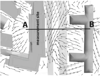
![Fig. 2 Schematic view over the measurement site and cross section through the measurement setup (adapted from [26])](https://thumb-eu.123doks.com/thumbv2/123doknet/14862892.636038/4.659.160.503.80.368/fig-schematic-measurement-cross-section-measurement-setup-adapted.webp)


Documents relatifs
We use our 3D model to calculate the thermal structure of WASP-43b assuming different chemical composition (ther- mochemical equilibrium and disequilibrium) and cloudy..
longues papilles adanales, des lobes dépourvus de soies margi- nales autour de la région spiraculaire et le dernier segment abdo- minal sans touffes de soies.. La
(Clinique Médicale 1) Chirurgie Thoracique et Cardiovasculaire Ophtalmologie Anesthésiologie - Réanimation Cardiologie Orthopédie - Traumatologie Médecine légale Pédiatrie
In analogy with direct measurements of the turbulent Reynolds stress (turbulent viscosity) that governs momentum transport, we have measured the turbulent electromotive force (emf)
In this paper, we offer a comprehensive investigation on the relative efficiency and effectiveness of various crackdown policies using a lab-in-the-field experiment with
Given that past research often related biological determinism to immutability beliefs rather than distinctiveness beliefs (Haslam & Levy, 2006; Hegarty, 2002), Study 2 included
(a) It was predicted that a higher aesthetic appeal of the device would lead to higher usability ratings and more positive emotions than a less aesthetically appealing device but
The magnetization measurements where performed on an automatic pulsed field magnetometer with a maximum field of 25 T and a pulse duration of 5 ms in the temperature range of 4.2
