Transport of SF 6 and 14 CO 2 in the atmospheric general circulation model ECHAM4

HAL Id: hal-03122981

https://hal.archives-ouvertes.fr/hal-03122981

Submitted on 3 May 2021

HAL is a multi-disciplinary open access

archive for the deposit and dissemination of

sci-entific research documents, whether they are

pub-lished or not. The documents may come from

teaching and research institutions in France or

L’archive ouverte pluridisciplinaire HAL, est

destinée au dépôt et à la diffusion de documents

scientifiques de niveau recherche, publiés ou non,

émanant des établissements d’enseignement et de

recherche français ou étrangers, des laboratoires

general circulation model ECHAM4

Erik Kjellström, Johann Feichter, Georg Hoffman

To cite this version:

Erik Kjellström, Johann Feichter, Georg Hoffman. Transport of SF 6 and 14 CO 2 in the atmospheric

general circulation model ECHAM4. Tellus B - Chemical and Physical Meteorology, Taylor & Francis,

2016, 52 (1), pp.1-18. �10.3402/tellusb.v52i1.16078�. �hal-03122981�

Full Terms & Conditions of access and use can be found at

ISSN: (Print) 1600-0889 (Online) Journal homepage: https://www.tandfonline.com/loi/zelb20

Transport of SF

₆

and

14

CO

₂

in the atmospheric

general circulation model ECHAM4

Erik Kjellström, Johann Feichter & Georg Hoffman

To cite this article:

Erik Kjellström, Johann Feichter & Georg Hoffman (2000) Transport of SF

and

CO

in the atmospheric general circulation model ECHAM4, Tellus B: Chemical and Physical

Meteorology, 52:1, 1-18, DOI: 10.3402/tellusb.v52i1.16078

To link to this article: https://doi.org/10.3402/tellusb.v52i1.16078

© 2000 The Author(s). Published by Taylor & Francis.

Published online: 15 Dec 2016.

Submit your article to this journal

Article views: 54

View related articles

Transport of SF

6

and

14CO

2

in the atmospheric general

circulation model ECHAM4

By ERIK KJELLSTRO¨ M1*, JOHANN FEICHTER2 and GEORG HOFFMAN3, 1Department of

Meteorology, Stockholm University, S-10691 Stockholm, Sweden;2Max-Planck Institute for Meteorology, Bundesstraße 55, D-20146 Hamburg, Germany;3L aboratoire des Sciences du Climat et de l’Environnement,

DSM, Orme des Merisiers, Bat. 703, piece 22 C.E. Saclay, F-91191 Gif-sur-Y vette Cedex, France (Manuscript received 23 July 1998; in final form 9 June 1999)

ABSTRACT

Two tracers, SF₆ with sources at the earth’s surface and 14CO₂ with a source in the lower stratosphere, are used to investigate the simulation of global scale transport in an atmospheric general circulation model. The simulated mixing ratios of SF

6in the troposphere are generally in close agreement to observations revealing a realistic description of the large scale tropospheric transport. The interhemispheric exchange time for SF

6is calculated to be 0.9 years, indicating a slightly too strong interhemispheric exchange. In the lowermost stratosphere the simulated vertical gradient of SF₆is in good agreement with observations within the 1st 4 to 5 km above the tropopause indicating that the flux from the troposphere to the lowermost stratosphere is captured by the model. On the other hand, downward transport of14CO₂from the stratosphere into the troposphere is found to be overestimated. From a comparison with observations it is concluded that it is the downward transport in the subtropics that is overestimated, at high latitudes the vertical gradients in the tropopause region are close to observations. Finally, the tracer tests show that the transport into the uppermost two levels, above 20 km, is underesti-mated as these levels serve as sponge layers and not as layers with a reasonable transport. Consequently, the tracer concentrations in that altitude interval are underestimated, by up to a factor 2.

1. Introduction chlorofluorocarbons, methane and sulfur species can, after entering the stratosphere, influence the local chemistry. The stratospheric ozone depletion In the last few decades an increasing interest in

and the production of sulfate aerosols in the Junge chemical species, man-made and natural, in the

layer around 20 km are two examples (World atmosphere has developed. The exchange of

chem-Meteorological Organization (WMO), 1994; ical species within both the troposphere and the

Crutzen, 1976). Downward transport of chemical stratosphere, and between them (stratosphere–

compounds from the stratosphere to the tropo-troposphere exchange — STE), is of crucial

impor-sphere, can be of importance for the chemistry in tance for the chemical balance in these reservoirs.

the troposphere (Wang et al., 1998) and maybe Chemical species of tropospheric origin, like

also a source of aerosol particles (Song et al., 1996). To study such fluxes of various tracers, * Corresponding author. Present affiliation:

atmospheric general circulation models (GCMs) Department of Earth, Atmosphere and Planetary

have often been used (Roelofs and Lelieveld, 1995; Sciences, Massachussetts Institute of Technology, Bldg.

Kjellstro¨m, 1998). However, these models have a 54-1726, Cambridge, MA 02140, USA.

which can lead to difficulties in calculating STE _{sphere make SF6 a suitable tracer for evaluating} tracer transport not only in the troposphere but that occurs on smaller scales.

Previous studies of the transport of chemical also into the lower stratosphere.

Radioactive14C was produced during the large tracers in global tracer transport models include

both short-lived tracers as 222Rn (Feichter and nuclear bomb tests mainly in the years 1961–62. 14C also has a natural cosmogenic source, but the Crutzen, 1990; Jacob et al., 1997) and long-lived

tracers as chlorofluorocarbons (Prather et al., excess14C produced by the bomb tests is a much stronger signal than the natural background pro-1987; Waugh et al., 1997). In this study we want

to address the question of how accurately a GCM, duction. Excess14C has been extensively used as tracer for ocean dynamics (Oeschger et al., 1975; with its limitations, can simulate STE and also

other transport processes like the interhemispheric Siegenthaler, 1983) and for the carbon exchange between ocean and atmosphere (e.g. Stuiver, 1980; exchange within the troposphere and the lower

stratosphere. The exchange processes at the tropo- Stuiver et al., 1981; Broecker et al., 1985; Hesshaimer et al., 1994).

pause are different from upward and downward

transport (Holton et al., 1995). Therefore, we Most of the14C from bomb tests was released in the altitude region between 20 and 30 km, investigate the transport of two long-lived tracers;

SF

6which has a surface source, and14CO2which mainly in the northern hemisphere. Therefore,14C is an attractive tracer to gain information on the was emitted into the stratosphere during

atmo-spheric nuclear bomb tests in the 1950s and 1960s. stratospheric transport and the STE. By compar-ing the simulated14C concentrations with surface Recently, SF

6was proposed as a powerful tracer

for evaluating transport in GCMs (Maiss et al., observations (Nydal and Lo¨vseth, 1996) of 14C in atmospheric CO2 (from hereafter the excess 1996). SF6 is of anthropogenic origin and emitted

at the surface, primarily in the northern hemi- radioactive14C is referred to as 14CO₂) we will use the14CO₂as a check for the STE as modelled sphere. An almost quadratic atmospheric increase

from 0.03 pptv between the first reported measure- by the ECHAM model. The seasonality of excess 14CO₂of about 200–100 per mil observed during ment in 1970 to 3.5 pptv in 1996 has been reported

by Maiss et al. (1996) and Geller et al. (1997). the first years after the test stop (1963–1965) in the northern hemisphere is of particular interest Chemical reactions of SF

6 with O(1D) and OH

have been reported to proceed very slowly since it allows inference on the seasonality of the STE.

(Ravishankara et al., 1993). They reported reac-tion rate coefficients of less than 1.8×10−14 cm3 molecules−1 s−1 for the O(1D)-reaction and less than 5.0×10−19 cm3 molecules−1 s−1 for the

OH-reaction. Also photolysis is very slow with 2. Model description

absorption only for wavelengths shorter than

130 nm (DeMore et al., 1997). Ravishankara et al. In order to simulate the transport of14CO₂and SF

6 we use the atmospheric general circulation (1993) concluded that the major destruction of

SF

6 is electron attachment in the mesosphere. model ECHAM4 (Roeckner et al., 1996). The model calculates transport of tracers using a semi-They estimated the atmospheric lifetime to be

3200 years with a lower limit at 580 years. Since Lagrangian scheme (Rasch and Williamson, 1990) for advection. Convective transport of tracers is stratospheric sinks are lacking the stratospheric

mixing ratios are determined only by the transport calculated with a mass-flux scheme (Tiedtke, 1989) which considers both updraft and downdraft mass time of air from the tropopause. From vertical

profiles of SF

6 the age of stratospheric air has fluxes and also entrainment and detrainment. An adjustment closure based on the convective avail-been determined (Harnisch et al., 1996; Patra

et al., 1997), above 25 km the lag in time, with able potential energy is used. Organized entrain-ment is assumed to depend on buoyancy, and the respect to the troposphere, was found to be

4.5 years for the tropics, 6 years for the mid- parameterization of organized detrainment is based on a cloud population hypothesis (Roeckner latitues and 10 years for the Arctic winter vortex.

The emission distribution, the steady increase with et al., 1996). The numerical formulation of the convective scheme has been altered in order to time, and the stability of SF

atmo-make the convective transport scheme strictly _{calculating SF6 emissions as in the TransCom2} experiment (Denning et al., 1999). The expression positive (Brinkop and Sausen, 1997).

The ECHAM4 model is run with a spectral from Levin and Hesshaimer (1996): triangular truncation at wave number 30 (T30)

E=0.2133(t−1990)+4.913, (1)

which corresponds to a Gaussian

longitude–lati-tude grid with a grid spacing of approximately where E is the emission in Gg SF

6per year and t is the time in years AD is used in this work. The 3.75°. The model uses a hybrid coordinate system

with 19 levels from the surface up to 10 hPa. horizontal distribution of the SF

6emissions, which is calculated from the electric power usage per Pressure levels are at approximately 1010, 995,

970, 920, 860, 780, 690, 595, 500, 410, 340, 250, country (UN Energy Statistic Yearbook, 1992), was provided by Martin Heimann (personal com-190, 140, 100, 70, 50, 30 and 10 hPa corresponding

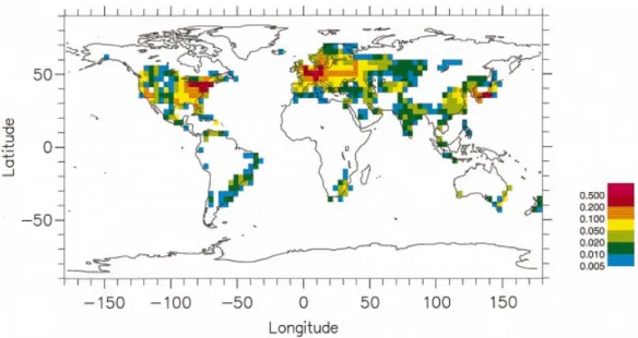
to midlayer altitudes of 0.03, 0.08, 0.4, 0.8, 1.4, 2.3, munication). About 95% of the emission is located in the northern hemisphere (Fig. 1). The SF6 3.2, 4.3, 5.6, 7.0, 8.6, 10.3, 12.1, 14.0, 16.0, 18.2,

20.6, 23.8 and 31.1 km above the surface. The time experiment is started with zero mixing ratios in October 1970.

step is 30 min. In the experiments the model is run for a 15-year period.

2.2. Initial distribution and sinks of14CO₂ 2.1. SF

6emissions On the basis of measurements done by the US

Atomic Energy Commission in the period from SF

6 is used in electrical equipment and metal

industries and is thought to be of entirely anthro- 1955 to 1970 and published in reports of the Health and Safety Laboratory (Telegadas, 1971; pogenic origin in the atmosphere (Maiss and

Levin, 1994). The SF

6-production has been Telegadas et al., 1972), Johnston (1989) established a 14CO₂ data set particularly adapted as initial increasing almost linearly since 1970 (Maiss et al.,

1996). The history of the SF

6-emission to the condition for testing atmospheric transport models. The initial14CO₂data are zonally uniform atmosphere has been estimated from the observed

atmospheric increase (Maiss and Levin, 1994). In and have a latitudinal resolution of 10°. The vertical resolution is 1 km between the surface and this experiment we use the same method for

Fig. 1. Horizontal distribution of SF₆emissions. The emissions are representative for January 1980. Unit: mg SF₆ m−2 yr−1.

3. Results and discussion

3.1. L ong-term trends

With linearly increasing emissions, the global average mixing ratio of SF6 in the model follows a quadratic increase with time given by

y(t)=0.0042t2+0.0228t−0.0211, (2)

where y(t) is the global average mixing ratio in pptv and t is the time (years) after 1970, Fig. 3. A quadratic increase with time of SF6 concentra-tions has been observed by Maiss et al. (1996) and Geller et al. (1997) for the time period Fig. 2. Initial distribution of excess14CO₂. Unit: per mil

1978–1996. A comparison of the simulated excess relative to the US National Institute of Standards

increase to the trend derived from the observations and Technology.

by Maiss et al. (1996) shows that the model lags behind since it starts with zero concentrations in 1970 (Fig. 3). Also, the simulated trend shows a 50 km height. The data describe the global

distri-faster increase than the trend derived by Maiss bution of excess14CO₂in October 1963 well after

et al. (1996) since our emissions increase at the Test Ban Treaty in 1962. At the end of 1963

a slightly higher rate. Because of these two the original bomb signal was already well mixed

differences the model results cannot directly be zonally. The initial data were linearly interpolated

compared with observed concentrations. The on the ECHAM4 grid, see Fig. 2.

difference between the simulated and observed The sink of atmospheric14CO₂is uptake at the

mixing ratios at a certain time varies between 0.1 earth’s surface, in vegetation and in sea surface

and 0.15 pptv during the time period 1973 to 1983. water. We follow the approach by Hesshaimer

In order to compare model simulated and et al. (1994) by introducing three boxes

repres-observed mixing ratios during that period the enting the terrestrial biosphere and a constant

average difference during those years, 0.13 pptv, is sink representing the oceans. The first biospheric

added to the model simulated mixing ratios. box represents fine roots, twigs and leaves (with a

Seen over a long time the14CO₂-content in the total carbon content of 105 Tg C), the second big

roots, stems and branches (675 Tg C) and the third slowly decomposing material from the other two biospheric boxes (1420 Tg C). The carbon in the three biospheric boxes is decomposed expo-nentially with a turn-over time of 3, 27 and 375 years respectively. Box 1 and 2 are directly coupled to the atmosphere with an input from the atmosphere adding up to 60 Tg C yr−1, corres-ponding to the net primary production. Box 3 gets its carbon input equally distributed from box 1 and 2, and ventilates into the atmosphere. For the flux of CO

2between the atmosphere and the oceans a gross flux of 60 Tg C yr−1 is assumed. The actual14CO₂flux between the different reser-voirs is calculated as the flux of CO2 times the

ratio between14C and 12C in the different reser- _{Fig. 3. Trend in global average SF}

6 mixing ratio. voirs. Only the long-time variations are considered _{Simulated trend as described by eq. (2) (full line) and} by this sink description, seasonal changes in the observed trend according to Maiss et al. (1996)

(dashed line). sinks are not accounted for.

model domain decreases exponentially with time the equator towards the poles in both hemispheres with the lowest mixing ratios in the northern with an e-folding time of seven years as a global

average (Fig. 4). Initially the simulated 14CO₂ hemisphere (Fig. 5c).

Also for 14CO₂ the simulated distribution is increases in the troposphere due to the downward

transport from the stratosphere. However, already zonally symmetric in the stratosphere on an annual mean basis (not shown). However, on after one year of the simulation, the tropospheric

14CO₂-content also decreases when the surface shorter timescales (weeks or months), large-scale features like the planetary waves appear in the sinks have become more important than the input

from the stratosphere. simulated distributions (this is also the case for

SF6). Unlike for SF6, the mixing ratios in the stratosphere are lowest at low latitudes revealing 3.2. Simulated geographical distributions

upward transport of14CO₂-poor tropospheric air at these latitudes. The tropospheric mixing ratios The simulated distribution of SF6 shows higher

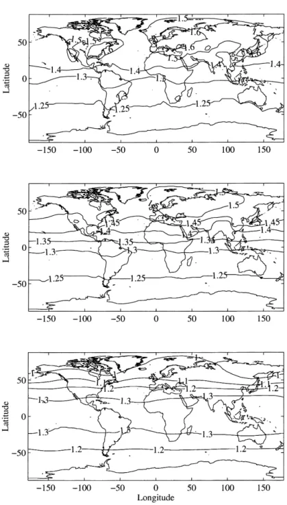
mixing ratios in the northern hemisphere than in are zonally uniform in general (Fig. 6). However, certain features are still present. First, higher the southern hemisphere, see Fig. 5a. Elevated

mixing ratios are found in, or downstream of, the mixing ratios are calculated in the northern hemi-sphere than in the southern hemihemi-sphere due to the industrialized regions. In the southern hemisphere,

where sources are almost absent, the predicted initial distribution of the stratospheric 14CO₂. Further, the mixing ratios are highest in the mixing ratios are lower and more uniform than in

the northern hemisphere. Above the boundary subtropics of the northern hemisphere troposphere where the combination of high stratospheric layer the distribution is zonally symmetric except

at mid and high northern latitudes (north of 40°N) 14CO₂-content, isentropic mixing of stratospheric air into the troposphere and downward motion is where the mixing ratios are slightly higher over

the Eurasian continent than over North America an effective source of tropospheric 14CO 2. Local maxima are also seen in the subtropics of the and Greenland (Fig. 5b). This difference is caused

by the distribution of the emissions with the southern hemisphere but not as strong as in the northern hemisphere since the stratospheric con-European sources being located further to the

north than the North American sources. At higher tent at these latitudes is smaller than at the corresponding northern latitudes.

tropospheric levels this difference decreases and above the tropopause level the annual mean is more zonally symmetric also at these latitudes. In

3.3. Interhemispheric exchange the stratosphere the concentration decreases with

height due to the slow mixing into these high The interhemispheric exchange time (_{tex), which} is a measure of the exchange between the hemi-levels. The stratospheric mixing ratios decline from

spheres, may be defined by

tex=(MNH−MSH)/FNH–SH, (3)

where M

NH and MSH are the tracer mass in the respective hemispheres, and FNH–SH is the net flux of the tracer from the northern to the southern hemisphere (Prather et al., 1987).

We calculate an interhemispheric exchange time of 0.9 years which is slightly lower than the 1.1 years calculated in the 2D-model by Levin and Hesshaimer (1996) and the 3D-model by Jacob et al. (1987) using85Kr. The simulated transport between the hemispheres is most efficient at the solstices when the intertropical convergence zone (ITCZ) is located at its northern or southern extreme (Fig. 7). Levin and Hesshaimer (1996) Fig. 4. Trend in global (full line), tropospheric (dashed

Fig. 5. Annual average distribution of SF

6from year 15 (corresponding to 1984) in the simulations. Lowest model level (top panel ), 850 hPa (middle panel ) and 100 hPa (lower panel ). Unit: pptv.

Fig. 6. Distribution of14CO₂at 700 hPa from January of the fourth year of the simulations (corresponding to 1966). Unit: per mil excess relative to the US National Institute of Standards and Technology.

the two hemispheres (Maiss et al., 1996; Levin and Hesshaimer, 1996 and Geller et al., 1997). In these studies the difference between the hemispheres was derived primarily from observations at the surface. As pointed out by Jacob et al. (1987) and Levin and Hesshaimer (1996); using the high concentrations of respectively 85Kr and SF₆ in the northern hemi-sphere boundary layer as representative for the northern hemisphere will lead to a too strong inter-hemispheric gradient and thereby to relatively long interhemispheric exchange times in simple box-models. 2- and 3-dimensional models take into account also the vertical distribution of the tracer, thereby reducing the interhemispheric gradient (Fig. 8) and calculating a shorter interhemispheric Fig. 7. Seasonal variation of the interhemispheric _{exchange time. Nevertheless, compared with} obser-exchange time as calculated in the model (dashed line).

vations the model simulated latitudinal distribution The corresponding values from Levin and Hesshaimer

shows a slightly weaker latitudinal gradient implying (1996) are included as a comparison (full line).

a somewhat too strong interhemispheric transport. Maiss and Brenninkmeijer (1998) derive expres-exchange time and found a slightly stronger

sea-sions for hemispheric trends of SF

6. Comparing sonal cycle than here, but unlike our results, they

their hemispheric trends show that the difference found no minimum in the interhemispheric

between the northern and southern hemispheres exchange time in the northern hemisphere summer

increase with 0.01 pptv yr−1 during the time (Fig. 7). This lack of a summer minimum is the

period 1970 to 1985. In this study an increase of main reason for why their annual average

inter-0.008 pptv yr−1 is calculated. The slower increase hemispheric exchange time is higher than ours, in

of the difference between the hemispheres this work a stronger interhemispheric exchange is

strengthens the notion of an overestimated inter-predicted also during northern hemisphere

hemispheric exchange. summer.

The simulated interhemispheric exchange time is

3.4. Seasonal variations considerably shorter than the 1.3–1.7 years that have

been estimated with two-box models using the The seasonal variations of SF

6depend only on the dynamics and transport of the model since observed difference in SF

provide a possibility of studying the seasonal behaviour of SF

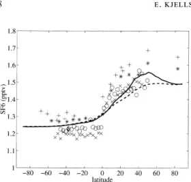
6 at a remote site. The model captures the main features of the seasonal cycle — the low mixing ratios in austral summer and the high mixing ratios in spring (Fig. 9). The seasonal cycle at these high latitudes lags with 6 to 7 months compared with the equatorial region. This lag corresponds to the simulated transport time of air from the equator to the South Pole region. The amplitude of the seasonal cycle at Neumayer is underestimated by almost a factor 2, a feature also noted by Levin and Hesshaimer (1996) with their 2D-model. Based on observations of 7Be, which is primarily of stratospheric origin, at Neumayer they claim that a too weak downward Fig. 8. Latitudinal distribution of SF₆. Simulated zonal

transport of stratospheric air may contribute to means; lowest model level (full line) and 850 hPa (dashed

their underestimate. Downward transport of stra-line). Oceanic shipboard measurements from Maiss et al.

tospheric air would give lower mixing ratios of (1996) and Geller et al. (1997) are plotted as: (+) the

Atlantic in November 1990, (1) the Atlantic in November _{SF6 but also higher mixing ratios of 14CO2 at the} 1993, (×) the Pacific Ocean in January–February 1994 _{surface. We calculate both 14CO}

2 and SF6to be and (#) the Atlantic in October–November 1994. All _{highest (lowest) in austral spring (summer). This} observational data have been scaled to July 1984

accord-coherence, between14CO_{2and SF6, indicates that} ing to Geller et al. (1997). The corresponding observation

the relatively low simulated SF

6mixing ratios in at Cape Grim is shown for comparison (§).

summer does not have to do with downward mixing of stratospheric air which is low in SF

6. Contributing to the too weak simulated seasonal there are no seasonal variations in the emissions.

In the boundary layer at high northern latitudes cycle at Neumayer could be a poor representation of the seasonal cycle of either the interhemispheric the simulated mixing ratios are higher in winter

than in summer (not shown). The higher ratios exchange (as discussed in Subsection 3.3) or the transport into mid and high southern latitudes. during winter are due to the more stable boundary

layers and also due to the northward transport from the source regions into the Arctic region during this season. The amplitude of this high latitude seasonal cycle is almost 5% of the detrended annual mean (i.e. the long-term trend discussed in Subsection 3.1 has been removed). The opposite seasonal variation can be seen in the free troposphere where mixing ratios are higher during summer due to convection. The strongest seasonal cycle of SF

6in the troposphere, with an amplitude of more than 10%, is simulated in the boundary layer of the equatorial region due to the movement of the ITCZ. In this region high mixing ratios are calculated in the northern hemi-sphere winter when the ITCZ is displaced to the

Fig. 9. Seasonal cycle of SF

6 at Neumayer, Antarctica south. At mid and high latitudes in the southern

(71°S, 8°W). The seasonal deviation from the average of hemisphere, where sources are almost absent, the

the last 8 years of the simulations is drawn as a dashed amplitude of the seasonal variations is less than _{line. The interannual variation is represented as the} sea-1%. _{sonal deviation from the average for each year (full lines).} Almost 10 years of high temporal resolution Observations from 1988 to 1993 (except February 1991

to February 1992) are from Maiss et al. (1996) (#). data from Neumayer in Antarctica (71°S, 8°W),

From the Neumayer data alone it is impossible to the observations with increasing altitude. At mid and high latitudes (polewards of 30°) the calcu-judge which is the most likely shortcoming in

the model. lated mixing ratios are systematically about 30%

lower than the observations at 10 km above the tropopause. In the tropics (equatorwards of 15°) 3.5. Comparison with SF

6observations — upward the underestimate is about 20% at 5 km above transport from the troposphere

the tropopause.

At higher stratospheric levels the underestimate Simulated SF

6-mixing ratios are compared with

the AIRSTREAM observations (Leifer, 1992) is even stronger. Compared with the observed SF6-profiles shown in Fig. 11, the model underesti-(Fig. 10). These observations cover a latitudinal

region between 75°N and 51°S over the Pacific mates the SF

6-content in the upper model domain by up to a factor of 2 at 30 km altitude. The Ocean and North America and a height range

from below the tropopause up to about 20 km. relatively better agreement between the 2 sound-ings from northern Sweden in January and The agreement between model and observations

in the lower stratosphere is within 10% up to 4 February is explained by the fact that the observa-tions were made inside the Arctic polar vortex or 5 km above the tropopause both in the tropics

and at mid and high latitudes. Above that level where air with very low SF

6 mixing ratios is sinking from higher levels. At lower altitudes a the simulated mixing ratios drop off faster than

Fig. 10. Comparison between observed SF

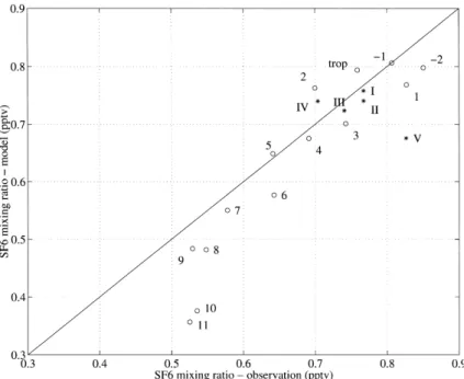
6 mixing ratios from project AIRSTREAM (Leifer et al., 1992) and corresponding simulated mixing ratios. The observations, which include 860 samples, cover the time period 1973–1983. The original data have been scaled depending on which laboratory that made the analysis, the scaling factors are: 1.18-HASL, 1.52-WSU and 1.76-OGC (Ingeborg Levin, personal communication). All the data, both model and observations, have been scaled to 1 January 1980 according to the Maiss et al. (1996) observed trend. 0.13 pptv has then been added to the simulated data (see text). The figure shows model versus observations where all data have been averaged and binned in altitude intervals of 1 km. Data representing the tropics (equatorwards of 15_{° latitude) are denoted with asteriscs and data representing high and mid latitudes (polewards of 30°) with} circles. The numbers indicate the altitude relative to the calculated or observed tropopause height in km. The tropopause height is defined as the lowest level at which the temperature lapse rate is 2 K km−1 and the average lapse rate between this level and any upper level within 2 km does not exceed 2 K km−1 (WMO, 1986).

Fig. 11. Vertical distributions of SF₆. Observed profiles from balloon soundings (Harnisch et al., 1996) (+) and simulated monthly means (full line). The profiles have been normalized by the average northern hemisphere tropo-spheric SF

6mixing ratio, taken from the trend derived by Geller et al. (1996), at the time of the sounding. The profiles are from (a) Hyderabad (India) in March, (b–e) Esrange (Sweden) in January ( b), February (c), March (d), March — outside the polar vortex (e) and (f ) Aire (France) in October.

qualitatively good agreement between model and _{concentration of SF6 in the troposphere exhibits} a relatively slow and steady increase the strato-observations is seen for all the soundings where

the lowermost observation in each sounding is spheric SF

6concentration is a function only of the age of stratospheric air (Hall and Plumb, 1994). from the troposphere. There are two reasons for

the unrealistic transport in the uppermost model Fig. 12 shows the distribution of time until the zonally averaged simulated mixing ratios of SF

6 layers: First, a damping of waves in the uppermost

model domain is included in the parameterization reach 0.3 pptv compared to the time when this level was first reached in the boundary layer of of horizontal diffusion to avoid reflection of waves

at the upper boundary (Roeckner et al., 1996). the source regions. About 1.5 years elapse between the time when the mixing ratios first reach this Second, no transport can occur across the upper

boundary of the model in contrast to the real level in the source regions until the same mixing ratios are simulated at the tropical tropopause. atmosphere in which vertical transport extends

into higher levels. This result is almost identical to what Hall and

Plumb (1994) found for a passive tracer with a The age of a stratospheric air parcel can be

defined as its mean transit time from the tropical northern mid latitude source. It is also consistent with the 0.8 years calculated by Waugh et al. tropopause (Hall and Plumb, 1994). Since the

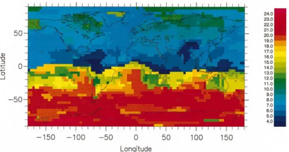
distribution is in fair agreement with the measure-ments by Elkins et al. (1996), though the latitud-inal gradients are somewhat too small (Waugh et al., 1997). The corresponding gradients in our simulation are about 1.5 and 0.5 years in the respective hemispheres. The small gradient in the southern hemisphere, which is obtained in all seasons, implies that our model has too fast pole-ward transport in the southern hemisphere. This too strong meridional transport is associated with the too strong meridional temperature gradient, between the tropics and the polar region in the model, which enhances the baroclinicity and Fig. 12. Zonally averaged time until the calculated thereby the horizontal mixing (Roeckner et al., mixing ratio of SF

6 reached 0.3 pptv compared to the 1996). At high northern latitudes we find a sea-time when this level was first reached in the boundary _{sonal cycle with a larger latitudinal gradient in} layer of the source regions. Unit: years.

age during winter and spring than in summer which could be attributed to the slower mixing into the polar vortex.

(1997) since they compared the time at the tropical tropopause with the global averaged trend at the surface derived by Geller et al. (1997). Above the

3.6. Comparison with14CO₂observations — tropical tropopause the calculated age of

strato-downward transport f rom the stratosphere spheric air increases with altitude in a similar way

as found by Hall and Plumb (1994) and by Waugh Observed vertical profiles of 14CO₂ from Johnston (1989) are compared with simulated et al. (1997). At higher altitudes the problem with

the upper boundary, as discussed in the previous zonal mean profiles at 70°N, 30°N, 9°N, and 42°S, Figs. 13, 14. The observations were carried out section, leads to lag times that are about twice as

long as in their modelling studies and as observed initially 4, and later 2×per year during the time period 1963–1970. As for SF

6, the agreement by Harnisch et al. (1996).

The model simulates lower ages in the strato- between calculated and observed mixing ratios in the stratosphere is best in the 1st 4 to 5 km above sphere of the southern hemisphere than in the

northern hemisphere indicating that the poleward the tropopause (corresponding to about 20 km in the tropics and 15 km in the mid-latitudes). The transport of air is stronger in the southern

hemi-sphere. This result is consistent with results from best agreement in the lower stratosphere and in the troposphere is found at 70°N while at lower Rosenlof and Holton (1993) when they calculate

the horizontal flux of air across an idealized latitudes concentrations in this altitude region are overestimated. This overestimation together with tropopause break between 100 and 200 hPa at 30°

latitude. They found this horizontal flux to be an underestimation at the height of the peak levels (Fig. 13) indicate a too rapid downward transport almost twice as large in the southern hemisphere

as in the northern hemisphere during December, of stratospheric 14CO₂. Further, the underesti-mated concentrations above the altitude of the January and February. However, our results are

in contrast to the observed age distributions peak levels suggest that the upward transport to the uppermost model layers is too weak.

derived from SF

6 observations by Elkins et al.

(1996) and modelled by Waugh et al. (1997). The From the stratospheric14CO₂-content reported by Telegadas (1971), Johnston (1989) estimated difference can be illustrated by the

interhemi-spheric difference in October for which Waugh the e-folding time of the global inventory of strato-spheric14CO₂to be 2.3 years from January 1963 et al. (1997) compare their results to the

measure-ments from Elkins et al. (1996). At 19.8 km they until October 1964, and 5.7 years between January 1965 and July 1966. The difference between calculate a latitudinal gradient in age of about

1 year between the equator and 30°N and almost the two time periods reflects the rapid removal of 14CO₂ from the lower stratosphere at the 2 years between the equator and 30°S. This age

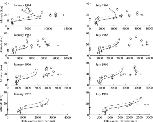
Fig. 13. Observed vertical profiles of14CO₂at 70°N (+) and 30°N (#) from Johnston, 1989. Corresponding simulated profiles from the model are shown as a solid line at 70°N and a dashed line at 30°N. The model tropopause level is indicated as× (70°N) and 1 (30°N) on the altitude axis.

beginning of the integration. At higher altitudes the our model (L19). In L39, the initial14CO₂-content also decreases too fast with an e-folding time of 14CO₂remained longer and it is that part of the

stratospheric 14CO₂ content which determines 1.3 years for the fist period (Land, 1999) similar to L19. This too fast decrease also in L39 indicates the lifetime in the latter period (Johnston, 1989).

We calculate corresponding lifetimes of 1.3 years that the vertical resolution is not the main problem unless an even higher vertical resolution is for the period between October 1963 and October

1964 and 5.2 years for the latter period. The rapid required. Nevertheless, during the first months of the simulation L39 performs better compared to decrease of stratospheric 14CO₂ at the beginning

of the simulation indicates a too strong flux to the observations implying that the vertical reso-lution has some impact on the simulations. The the troposphere. One possible reason for this too

strong downward flux of stratospheric air could rather good agreement between our model and the observations in the latter period does not be the coarse vertical resolution in the model. In

order to investigate the influence of vertical reso- imply that the calculated transport to the tropo-sphere is better, it merely reflects the combination lution we have compared our results with a version

of the ECHAM4 model that has 39 vertical levels of a fast downward transport from the lowermost stratosphere and a slow vertical transport in the between the surface and 10 hPa (model version

L39). In the tropopause region L39 has a vertical uppermost model domain as discussed in the previous section.

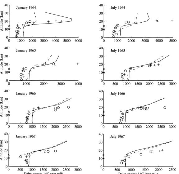
Fig. 14. Observed vertical profiles of14CO₂at 9°N (+) and 42°S (#) from Johnston, 1989. Corresponding simulated profiles from the model are shown as a solid line at 9°N and a dashed line at 42°S. The model tropopause level is indicated as× (9°N) and 1 (42°S) on the altitude axis.

Compared with the observed profiles from which implies a too strong downward flux from the stratosphere. Further, the overestimation in Johnston (1989) the simulated mixing ratios of

14CO₂in the lowermost stratosphere become too the southern hemisphere troposphere and lower-most stratosphere (Fig. 14) suggests that the inter-high within a few months after the start of the

simulation (Figs. 13, 14). This pattern, which is hemispheric transport is too strong. A too strong downward tracer flux is consistent with calcula-common to all latitudes except 70°N where the

agreement between observations and model results tions of air mass flux across the tropopause in a previous model version ECHAM3 by Grewe and is good throughout the simulations, indicates that

the downward transport of14CO₂is overestimated Dameris (1996): they found that the model over-estimates the downward flux at 30°N and 40°S at lower latitudes. Both at 30°N and especially at

42°S, also the tropospheric mixing ratios in the with a factor of approximately 1.5 to 2. The better agreement to observations that we find at higher first months of the simulations are overestimated,

latitudes (70°N) is consistent with the results by tions. Also the northern hemisphere tropics experi-ence the maximum at an early stage due to Kentrachos et al. (1999) who use the same model

as in this study applied to a specific synoptic northerly winds during the winter when the peak first reaches the surface, later on the ITCZ moves situation over Europe. They conclude that the

model is able to predict intrusions of stratospheric northwards passing these regions. Within 1 year the entire northern hemisphere has experienced O

3 into the troposphere in a realistic way. A

possible reason for the too strong downward the maximum 14CO₂ concentration. The pattern in the southern hemisphere is similar, with the transport at lower latitudes could be insufficient

horizontal resolution. Siegmund et al. (1996) use first maximum at the surface predicted in the subtropics after a few months. The entire analysed meteorological data to investigate the

STE. In going from a horizontal resolution of 0.5° southern hemisphere is reached by the first max-imum within a year. Fig. 15, on the other hand, to 3.75° they find that the maximum downward

flux close to 30°N increase with almost a factor 3. shows that the time of the overall highest concen-trations is more than 1 year for most of the At mid and high latitudes, on the other hand, they

find the average cross tropospheric flux to be southern hemisphere. The higher concentrations of the 2nd year of the simulation, are due to much less sensitive to the horizontal resolution.

Also contributing to a too strong downward flux transport of 14CO₂-rich air from the northern hemisphere. Within two years also remote parts could be a too strong horizontal isentropic mixing

(see last paragraph of Subsection 3.5) followed by of the southern hemisphere are reached by the peak in the14CO₂signal.

downward motion in the subtropics.

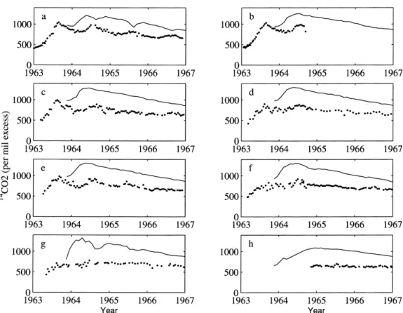
At the surface of the northern hemisphere the The absolute peak levels at tropopause levels in the northern hemisphere were observed already in model predicts a rapid increase in 14CO₂during

the first year of the simulation. Fig. 15 shows the January and April 1963 (Johnston, 1989) which is prior to the period simulated here. During the time when the maximum14CO₂concentration at

the model level closest to the surface is reached. first years after this time a clear seasonal cycle has been found at some of the northern hemisphere The fastest downward transport of14CO₂is

pre-dicted in the subtropics of the northern hemisphere surface stations (Nydal and Lo¨vseth, 1996) (Fig. 16). Maximum concentrations are observed where the maximum at the surface is reached

within 4 to 6 months from the start of the simula- during summer indicating seasonal input from the

Fig. 16. Observed (dots) and simulated (full line) evolution of14CO₂at surface stations. The observations are from Nydal and Lo¨vseth (1996): (a) Fruholmen, Norway (78°04N, 13°38E), (b) Lindesnes, Norway (57°59N, 07°04E), (c) Santiago de Compostela, Spain (42°53N, 08°26W), (d) Izana, Spain (28°N, 16°30W), (e) Mas Palomas, Spain (27°45N, 15°40W), (f ) Dakar (1963–64) and Dakar-Fann (1964–68), Senegal (14°40N, 17°20W), (g) Debre Zeit, Ethiopia (8_{°40N, 38°58E) and (h) Fianarantsoa, Madagascar (21°27S, 47°05E). Unit: per mil excess relative to the} NIST standard.

stratosphere of14CO₂(Nydal and Lo¨vseth, 1983). tropospheric 14CO₂ content efficiently masks the seasonal signal from stratospheric downward The model simulated maxima, on the other hand,

occur up to 4 months earlier than observed. This transport in the subsequent years of the simula-tion. Fig. 16 also shows that the14CO₂ concentra-lead of the model before the observations indicates

that the simulated downward transport is too fast. tions decrease too rapidly at all observational stations. This rapid decrease indicates that the Further, the model overestimates the ground level

14CO₂concentrations at the time of the maximum global sink terms are overestimated in the model, a feature also discussed by Hesshaimer et al. compared with the observed maximum. This

over-estimate, which is more pronounced at the stations (1994). located closer to the equator, also supports the

notion of a too strong subtropical downward

transport in the model. The lack of a clear seasonal 4. Summary and conclusions

cycle in the model results is probably due to the

too rapid initial downward mixing of 14CO₂. The ECHAM4 model is able to simulate the main features of the observed atmospheric SF

6 Already after a few months of the simulation the

tropospheric content of 14CO₂ is much higher pattern, such as the vertical and latitudinal distribution in the troposphere and lowermost than the stratospheric content (Fig. 4). The high

stratosphere and the phase of the seasonal cycle indicates that the interhemispheric transport in the troposphere is too strong. Also indicative of a at a remote observational site in the southern

hemisphere. A comparison of the simulated ver- too strong interhemispheric exchange is the too rapid buildup of stratospheric and tropospheric tical gradient of SF6 in the tropopause region with

observations shows that the model captures the 14CO₂compared with observations at 40°S. It is clearly illustrated how the treatment of the stratospheric decline in mixing ratio with

increas-ing altitude in the first 4 or 5 km above the upper boundary, with a strong damping and no transport across it, hampers a realistic simulation tropopause. The ability of the model to predict

the cross-tropopause gradient implies that the of tracer transport at the uppermost model levels. Especially above 20 km the mixing ratios of both simulated upward net flux of SF6 across the

tropo-pause level is realistic. SF

6 and14CO2are underestimated with up to a factor 2 compared with a few measurements that The global stratospheric 14CO₂ content

decreases rapidly at the beginning of the simula- are available at these levels. From a comparison with observations (Elkins et al., 1997) and previous tion. The calculated e-folding time during the first

year is 1.3 years which is shorter than what has simulations (Waugh et al., 1997) of the age of stratospheric air, it is concluded that the model been deduced from observations indicating a too

strong downward transport of14CO₂. The model simulates a too strong polewards transport of SF 6 in the southern hemisphere close to 20 km height. predicts maximum surface concentrations leading

the observations with up to 4 months at low latitude sites in Africa and southernmost Europe.

At high latitudes the simulated temporal evolution 5. Acknowledgements

is in better agreement with observations both at

the surface and in the free troposphere. Therefore, The authors wants to thank Martin Heimann for providing emission data for SF6. We are it is concluded that the overestimated downward

transport of 14CO₂is concentrated mainly to the grateful to Bob Leifers who provided EML data and to Mannfred Maiss and Ingeborg Levin who subtropics.

The calculated interhemispheric exchange time provided correction factors for the EML data. Further we are grateful to Henning Rodhe, Eliza of SF

6of 0.9 years is slightly lower than previous

estimates. This fact together with the too slow Manzini and Christine Land for constructive discussions and suggestions on the manuscript. increase in the gradient between the hemispheres

REFERENCES

Brinkop, S. and Sausen, R. 1997. A finite difference port and concentration of SF₆: a model intercompar-ison study (Transcom 2). T ellus 51, 266–297. approximation for convective transports which

main-tains positive tracer concentrations. Beitr. Phys. Elkins, J. W., Fahey, D. W., Gilligan, J. M., Dutton, G. S., Baring, T. J., Volk, C. M., Dunn, R. E., Myers, Atmosph. 70, 245–248.

Broecker, W., Peng, T.-H., Ostlund, G. and Stuiver, M. R. C., Montzka, S. A., Wamsley, P. R., Hayden, A. H., Butler, J. H., Thompson, T. M., Swanson, T. H., 1985. The distribution of bomb radiocarbon in the

ocean. J. Geophys. Res. 90, 6953–6970. Dlugokencky, E. J., Novelli, P. C., Hurst, D. F., Lobert, J. M., Ciciora, S. J., McLaughlin, R. J., Thompson, Crutzen, P. 1976. The possible importance of CSO for

the sulfate layer of the stratosphere. Geophys. Res. T. L., Winkler, R. H., Fraser, P. J., Steele, L. D. and Lucarelli, M. P. 1996. Airborne gas chromatograph L ett. 3, 73–76.

DeMore, W. B., Sander, S. P., Golden, D. M., Hampson, for in situ measurements of long-lived species in the upper troposphere and lower stratosphere. Geophys. R. F., Kurylo, M. J., Howard, C. J., Ravishankara,

A. R., Kolb, C. E. and Molina, M. J. 1997. Chemical Res. L ett. 23, 347–350.

Feichter, J. and Crutzen, P. J. 1990. Parameterization of kinetics and photochemical data for use in stratosphere

modeling. Evaluation number 12. JPL publication 97-4, vertical transport due to deep cumulus convection in a global transport model and its evaluation with Jet Propulsion Laboratory, Pasadena, Calif., USA.

Denning, A. S., Holzer, M., Gurney, K. R., Heimann, M., 222Radon measurements. T ellus 42, 100–117. Geller, L. S., Elkins, J. W., Lobert, J. M., Clarke, A. D., Law, R. M., Rayner, P. R., Fung, I. Y., Fan, S.-M.,

Taguchi, S., Friedlingstein, P., Balkanski, Y., Taylor, J., Hurst, D. F., Butler, J. H. and Myers, R. C. 1997. Tropospheric SF

6: observed latitudinal distribution Maiss, M. and Levin, I. 1999. Three-dimensional

trans-and trends, derived emissions trans-and interhemispheric observed passive tracer distributions of85Kr and sulfur hexafluoride (SF

6). J. Geophys. Res. 101, 16745–16755. exchange time. Geophys. Res. L ett. 24, 675–678.

Grewe, V. and Dameris, M. 1996. The large-scale mass- Maiss, M. and Levin, I. 1994. Global increase of SF 6 observed in the atmosphere. Geophys. Res. L ett. 21, exchange between stratosphere and troposphere in the

ECHAM3 model. In Staniforth, A. (ed.): Research 569–572.

Maiss, M., Steele, P., Francey, R. J., Fraser, P. J., Langen-activities in atmospheric and oceanic modelling. CAS/

JSC working group on numerical experimentation. felds, R. L., Trivett, N. B. A. and Levin, I. 1996. Sulfur hexafluoride — a powerful new atmospheric tracer. Report No. 23 WMO/TD No. 734.7.21–7.22, Geneva,

Switzerland. Atmos. Environ. 30, 1621–1629.

Maiss, M. and Brenninkmeijer, C. A. M. 1998. Atmo-Hall, T. M. and Plumb, R. A. 1994. Age as a diagnostic

of stratospheric transport. J. Geophys. Res. 99, spheric SF

6 trends, sources and prospects. Environ. Sci. T echnol. 32, 3077–3086.

1059–1070.

Harnisch, J., Borchers, R., Fabian, P. and Maiss, M. Nydal, R. and Lo¨vseth, K. 1983. Tracing bomb14C in the atmosphere 1962–1980. J. Geophys. Res. 88, 1996. Tropospheric trends for CF

4 and C2F6 since

1982 derived from SF₆dated stratospheric air. Geo- 3621–3642.

Nydal, R. and Lo¨vseth, K. 1996. Carbon-14 measurements phys. Res. L ett. 23, 1099–1102.

Hesshaimer, V., Heimann, M. and Levin, I. 1994. in atmospheric CO

2from northern and southern hemi-sphere sites, 1962–1993. ORNL/CDIAC-93, NDP-057. Radiocarbon evidence for a smaller oceanic carbon

dioxide sink than previously believed. Nature 370, Carbon Dioxide information analysis center, Oak Ridge National Laboratory, Oak Ridge, Tennessee, 201–203.

Holton, J. R., Haynes, P. H., McIntyre, M. E., Douglas, USA, 67 pp.

Oeschger, H., Siegenthaler, U., Schotterer, U. and Gugel-A. R., Rood, R. B. and Pfister, L., 1995. Stratosphere–

troposphere exchange. Rev. Geophys. 33, 403–439. mann, A. 1975. A box diffusion model to study the carbon dioxide exchange in nature. T ellus 27, 168–192. Jacob, D. J., Prather, M. J., Wofsy, S. C. and McElroy,

M. B. 1987. Atmospheric distribution of85Kr simu- Patra, P. K., Lal, S., Subbaraya, B. H., Jackman, C. H. and Rajaratnam, P. 1997. Observed vertical profile of lated with a general circulation model. J. Geophys.

Res. 92, 6614–6626. sulphur hexafluoride (SF₆) and its atmospheric applications. J. Geophys. Res. 102, 8855–8859. Jacob, D. J., Prather, M. J., Rasch, P. J., Shia, R.-L.,

Balkanski, Y. J., Beagley, S. R., Bergmann, D. J., Black- Prather, M., McElroy, M., Wofsy, S., Russell, G. and Rind, D. 1987. Chemistry of the global troposphere: shear, W. T., Brown, M., Chiba, M., Chipperfield,

M. P., de Grandpre´, J., Dignon, J. E., Feichter, J., Fluorocarbons as tracers of air motions. J. Geophys. Res. 92, 6579–6613.

Genthon, C., Grose, W. L., Kasibathla, P. S.,

Ko¨hler, I., Kritz, M. A., Law, K., Penner, J. E., Rasch, P. and Williamson, D. 1990. Computational aspects of moisture transport in global models of the Ramonet, M., Reeves, C. E., Rotman, D. A., Stockwell,

D. Z., van Velthoven, P. F. J., Verver, G., Wild, O., atmosphere. Q. J. R. Meteorol. Soc. 116, 1071–1090. Ravishankara, A. R., Solomon, S., Turnipseed, A. A. and Yang, H. and Zimmermann, P. 1997. Evaluation and

intercomparison of global atmospheric transport Warren, R. F. 1993. Atmospheric lifetimes of long-lived halogenated species. Science 259, 194–199. models using 222Rn and other short-lived tracers.

J. Geophys. Res. 102, 5953–5970. Roeckner, E., Arpe, K., Bengtsson, L., Christoph, M., Claussen, M., Du¨menil, L., Esch, M., Giorgetta, M., Johnston, H. 1989. Evaluation of excess carbon 14 and

strontium 90 data for suitability to test two-dimen- Schlese, U. and Schulzweida, U. 1996. T he atmospheric general circulation model ECHAM-4: Model descrip-sional stratospheric models. J. Geophys. Res. 94,

18485–18493. tion and simulation of present-day climate. Report no. 218, Max-Planck-Institute for Meteorology, Ham-Kentarchos, A. S., Roelofs, G. J. and Lelieveld, J. 1999.

Model study of a stratospheric intrusion event at lower burg, Germany.

Roelofs, G. and Lelieveld, J. 1995. Distribution and midlatitudes associated with the development of a

cutoff low. J. Geophys. Res. 104, 1717–1727. budget of O₃ in the troposphere calculated with a chemistry general circulation model. J. Geophys. Res. Kjellstro¨m, E. 1998. A three-dimensional global model

study of carbonyl sulfide in the troposphere and the 100, 20983–20998.

Rosenlof, K. and Holton, J. 1993. Estimates of the strato-lower stratosphere. J. Atmos. Chem. 29, 151–172.

Land, C. 1999. Untersuchungen zum globalen Spuren- spheric residual circulation using the downward control principle. J. Geophys. Res. 98, 10465–10479. stoVtransport mit dem Atmosphaerenmodell

ECH-AM4.L 39(DL R). PhD Thesis, University of Munich, Siegenthaler, U. 1983. Uptake of excess CO₂by an out-crop-diffusion model of the ocean. J. Geophys. Res. 88, Germany.

Leifer, R. 1992. Project AIRST REAM: T race gas final 3599–3608.

Siegmund, P. C., van Velthoven, P. F. J. and Kelder, H., report. USDOE Report EML-549, New York, USA.

Levin, I. and Hesshaimer, V. 1996. Refining of atmo- 1996. Cross-tropopause transport in the extratropical northern winter hemisphere diagnosed from high-spheric transport model entries by the globally

resolution ECMWF data. Q. J. R. Meteorol. Soc. 122, Safety Lab., US Atomic Energy Comm., Washington, DC, USA, report 246.

1921–1941.

Song, N., Starr, D., Wuebbles, D., Williams, A. and Tiedtke, M. 1989. A comprehensive mass flux scheme for cumulus parameterization in large-scale models. Mon. Larson, S. 1996. Volcanic aerosols and interannual

variation of high clouds. Geophys. Res. L ett. 23, Wea. Rev. 117, 1779–1800.

Wang, Y., Jacob, D. J. and Logan, J. A. 1998. Global 2657–2660.

Steil, B., Dameris, M., Bru¨hl, C., Crutzen, P. J., Grewe, V., simulation of tropospheric O

3−NOx− hydrocarbon chemistry (3). Origin of tropospheric O

3 and effects Ponater, M. and Sausen, R. 1997. Development of a

chemistry module for GCMs: First results of a multi- of nonmethane hydrocarbons. J. Geophys. Res. 103, 10757–10767.

annual integration. Annales Geophysical 16, 205–228.

Stuiver, M. 1980.14C distribution in the Atlantic Ocean. Waugh, D. W., Hall, T. M., Randel, W. J., Rasch, P. J., Boville, B. A., Boering, K. A., Wofsy, S. C., Daube, J. Geophys. Res. 85, 2711–2718.

Stuiver, M., Ostlund, H. G. and McConnaughey, T. A. B. C., Elkins, J. W., Fahey, D. W., Dutton, G. S., Volk, C. M. and Vohralik, P. F. 1997. Three-dimensional 1981. GEOSECS Atlantic and Pacific14C distribution.

In: Carbon cycle modelling, B. Bolin (ed.) John Wiley, simulations of long-lived tracers using winds from MACCM2. J. Geophys. Res. 102, 21493–21513. New York, USA, pp. 201–221.

Telegadas, K. 1971. T he seasonal stratospheric distribu- World Meteorological Organization (WMO). 1994. Sci-entific assessment of ozone depletion. Report 37, Global tion and inventory of carbon-14 f rom March 1955 to

July 1969. Health and Safety Lab, U.S. Atomic Energy ozone research and monitoring project. Geneva, Switzerland.

Comm., Washington, DC, USA, Report 243.

Telegadas, K., Gray, J., Sowl, R. E. and Ashenfelter, T. E. World Meteorological Organization (WMO). 1986. Atmospheric ozone 1985: Report 16, Global ozone 1972. Carbon-14 measurements in the stratosphere from