HAL Id: hal-03044144
https://hal.inria.fr/hal-03044144
Submitted on 7 Dec 2020
HAL is a multi-disciplinary open access
archive for the deposit and dissemination of
sci-entific research documents, whether they are
pub-lished or not. The documents may come from
teaching and research institutions in France or
abroad, or from public or private research centers.
L’archive ouverte pluridisciplinaire HAL, est
destinée au dépôt et à la diffusion de documents
scientifiques de niveau recherche, publiés ou non,
émanant des établissements d’enseignement et de
recherche français ou étrangers, des laboratoires
publics ou privés.
How to deal with missing data in supervised deep
learning?
Niels Ipsen, Pierre-Alexandre Mattei, Jes Frellsen
To cite this version:
Niels Ipsen, Pierre-Alexandre Mattei, Jes Frellsen. How to deal with missing data in supervised deep
learning?. Artemiss - ICML Workshop on the Art of Learning with Missing Values, Jul 2020, Vienne,
Austria. �hal-03044144�
Niels Bruun Ipsen1 Pierre-Alexandre Mattei* 2 Jes Frellsen* 1
Abstract
The issue of missing data in supervised learn-ing has been largely overlooked, especially in the deep learning community. We investigate strate-gies to adapt neural architectures to handle miss-ing values. Here, we focus on regression and classification problems where the features are as-sumed to be missing at random. Of particular interest are schemes that allow to reuse as-is a neural discriminative architecture. One scheme involves imputing the missing values with learn-able constants. We propose a second novel ap-proach that leverages recent advances in deep gen-erative modelling. More precisely, a deep latent variable model can be learned jointly with the discriminative model, using importance-weighted variational inference in an end-to-end way. This hybrid approach, which mimics multiple imputa-tion, also allows to impute the data, by relying on both the discriminative and the generative model. We also discuss ways of using a pre-trained gen-erative model to train the discriminative one. In domains where powerful deep generative models are available, the hybrid approach leads to large performance gains.
1. Introduction
Missing data affects data analysis across a wide range of domains and the sources of missing spans an equally wide range. Recently deep latent variable models (DLVMs,
Kingma & Welling,2013;Rezende et al.,2014) have been applied to missing data problems in an unsupervised set-ting (e.g. Rezende et al.,2014;Nazabal et al.,2018;Ma et al.,2018;2019;Ivanov et al.,2019;Mattei & Frellsen,
*
Equal contribution 1Department of Applied Mathematics and Computer Science, Technical University of Denmark, Denmark
2
Universit´e Cˆote d’Azur, Inria (Maasai project-team), Laboratoire J.A. Dieudonn´e, UMR CNRS 7351, France. Correspondence to: Niels Bruun Ipsen <[email protected]>, Pierre-Alexandre Mattei <[email protected]>, Jes Frellsen <[email protected]>. Presented at the first Workshop on the Art of Learning with Missing Values (Artemiss) hosted by the37th
International Conference on Machine Learning (ICML).Copyright 2020 by the author(s).
2018;2019;Yoon et al.,2018;Ipsen et al.,2020), while the supervised setting has not seen the same recent atten-tion. The progress in the unsupervised setting is focused on inference and imputation in a joint model over features with missing values and can be useful as an imputation step before a discriminative model. However, this approach is not necessarily optimal in terms of minimizing a prediction error.
We propose and investigate strategies for handling missing data in the supervised learning setting, while keeping any existing discriminative neural architecture as is, by inspect-ing how learninspect-ing curves depend on the chosen strategy. Our main contribution is a joint DLVM and discriminative model that can be trained using importance weighted variational inference.
1.1. Previous work
A recent attempt to handle missing data in discriminative models was done by´Smieja et al.(2018), where a Gaussian mixture model (GMM) is used as a preamble to a discrimi-native neural network. The GMM and discrimidiscrimi-native model are trained jointly, and in place of any missing values the activation of the corresponding input neuron is set to the average activation over the GMM conditioned on observed values. Yi et al.(2019) tackled the issue of sparsity, and specifically large variations in sparsity, by introducing spar-sity normalization. This handles issues of model output covarying with the sparsity level in the input. However, it does not address the information loss due to the missing process.Ma et al.(2018) used a permutation invariant setup to avoid imputing missing data in the input of a variational autoencoder. This approach can be readily extended to the supervised setting, using the permutation invariant setup as a modified input layer.
A review of approaches to handling missing data in (non-deep) supervised learning was given byJosse et al.(2019). Here it is shown that under some assumptions, mean im-putation is consistent in the supervised setting.Le Morvan et al.(2020) investigated the case of a linear predictor on covariates with missing data, showing that in the presence of missing, the optimal predictor may not be linear and how constant imputation of each feature can be optimized with regards to the model loss.
2. Background and notation
Rubin(1976) introduced the framework used for describing missing processes and their relation to the observed and missing data. Le Morvan et al.(2020) andSeaman et al.
(2013) have pointed out some shortcomings in the way this framework and notation are often used. We will use a notation along the lines ofLe Morvan et al.(2020) here. Assume we have a data matrix X = (x1, . . . , xn)|∈ Xn
that contain n i.i.d. copies of the random variable x ∈ X , where X = X1× · · · × Xpis a p-dimensional feature space.
There is a response matrix Y = (y1, . . . , yn) ∈ Ynthat
contains copies of the corresponding (possibly vector val-ued) response variable y ∈ Y. A missing process obscures parts of x resulting in the mask variable s ∈ {0, 1}p. The positions of observed entries in the data matrix X are con-tained in a mask matrix S = (s1, . . . , sn)| ∈ {0, 1}n×p
such that sij = ( 1 if xij observed, 0 if xij missing. (1) Then the observed data is
˜
X = X S + na (1 − S), (2) where is the Hadamard product and missing values are represented by na, defining na · xij= na and na · 0 = 0.
We let obs(s) denote the non-zero entries of s and miss(s) denote the zero-entries of s, such that xobs(s)are all the
observed elements of x and xmiss(s) are all the missing
elements of x. For simplicity we will omit the s and write xobs, xmissrespectively, whenever the context is clear.
We distinguish between the random variables (xobs, xmiss)
and the strategies used to turn realisations of xobsinto com-plete input vectors. Specifically an imputation function ι is used ι(xobs) ∈ X , such that ι(xobs)obs= xobs.
Finally, the goal is to minimize the prediction error by max-imizing the discriminative log-likelihood
`(φ) =
n
X
i=1
log pφ(yi|xobsi , si). (3)
3. Training deep supervised models with
missing data
We wish to compare different strategies to handling missing data in supervised deep learning, specifically a convolutional neural network for classification on images. The strategies are
• 0-imputation, • learnable imputation,
• concatenation of information in separate channels, • three different strategies for using a DLVM with a
discriminative model, M1, M2 and M3 respectively. We describe these approaches in the sections below. 3.1. Zero imputation
A simple version of constant imputation is 0-imputation, which has the intuitive appeal that the activation from the input node is zeroed out (absent). The input to the discrimi-native model is given by
ι0(xobs) = x s + 0 (1 − s). (4)
3.2. Learnable imputation
In the unsupervised setting constant imputation biases marginal and joint distributions, butJosse et al.(2019) have shown that mean imputation can be consistent in the super-vised setting. Furthermore,Le Morvan et al.(2020) noted that the constants can be optimized with respect to the model loss. This is the approach we take here, defining learnable parameters λ ∈ X to be inserted in place of the missing data, so that
ιλ(xobs) = x s + λ (1 − s). (5)
3.3. Concatenation in separate channels
In this work we are using a convolutional neural network for classification, so a straightforward way to merge information is to put it in separate channels in the input layer. We concatenate the following information: ι0(xobs),
λ and s. In multilayer perceptrons this could instead be done by concatenating information side by side.
3.4. Discriminative approaches using DLVMs
Here we explore how the recent progress made in apply-ing DLVMs to missapply-ing data problems can be utilized in the supervised learning setting. We take three different approaches:
• M1: We propose a joint generative and discriminative model, where a joint objective (equation (9)) ensures end-to-end training (figure1a).
• M2: The model is the same as M1, but the generative model is first pre-trained and fixed, and then the dis-criminative model is trained using the joint objective. • M3: The dataset imputed by a generative model
(fig-ure 1b) is given as input to a discriminative model (figure1c).
z x y θ φ γ N (a) z x θ γ N (b) x y φ N (c)
Figure 1. (a) Graphical model of M1 and M2. For M1 the parame-ters (θ, φ, γ) are learnt jointly using the objective in equation (9). For M2, θ and γ are found by pre-training the generative part of the model, then held fixed while learning φ using the joint loss. (b) and (c) show the approach in M3; the connection between the generative and discriminative model is severed, the DLVM is trained separately and used to generate a fully observed dataset as input to the discriminative model.
In all three approaches the generative parts are identical and the discriminative parts are identical. For the genera-tive part, our choice of DLVM is the MIWAE (Mattei & Frellsen,2019), based on importance weighted variational inference. Therefore the single imputations used to impute a full dataset are generated using self-normalized impor-tance sampling. With the joint objective, we can utilize self-normalized importance sampling as well, but instead of weighting samples from the generative part of the model to get imputations, we are weighting the predictions.
There are subtle distinctions between imputing a fixed dataset for the discriminative model (M3), training the dis-criminative model with the joint objective (M2) and training both the generative and discriminative model using the joint objective (M1). In M1 during training, the generative part of the model is tuned to improve the discriminative loss. In M1 and M2 importance weighted samples from the genera-tive part of the model are fed to the discriminagenera-tive model in place for the missing values, mimicking multiple imputation, where the class probabilities for each sample are importance weighted to give one final classification.
3.4.1. LOSS DERIVATION
In this section, we will derive the loss for inference in the joint model from figure 1a. The joint distribution p(y, xobs, xmiss, z) over class labels, observed and missing
covariates and latent variables can be factorized as
p(z)p(xobs|z)p(xmiss|z)p(y|xobs, xmiss), (6)
where we assumed that the conditional distribution of x can be fully factorized as p(x|z) =Q
jp(xj|z).
The likelihood of the observed data p(y, xobs) is equal to
Z Z
p(z)p(xobs|z)p(xmiss|z)p(y|xobs, xmiss) dxmissdz. (7) These integrals are usually analytically intractable. To ap-proach them, we build on amortized importance-weighted variational inference (Burda et al.,2016). Indeed, the likeli-hood can be estimated using importance sampling
p(y, xobs) ≈ 1
K
K
X
i=1
p(zk)p(xobs|zk)p(y|xobs, xmissk )
q(zk|xobs, s)
, (8) where q(zk|xobs, s) is the variational distribution (learnable
proposal) and (zk, xmissk )k∈{1,...,K}are i.i.d. samples from
p(xmiss|z)q(z|xobs, s). This leads to the following lower
bound of the log-likelihood:
LK = E log 1 K K X k=1
p(zk)p(xobs|zk)p(y|xobs, xmissk )
q(zk|xobs, s) . (9)
We note that whileIpsen et al.(2020) address a very dif-ferent problem, modelling data with values missing not at random, they assume the same independence structure as in figure1abut with mask instead of label and obtain a bound with the same structure as equation (9).
Remark. If a data point is fully observed, the loss is then simply LK= log p(y|x) + E log 1 K K X i=1 p(zk)p(x|zk) q(zk|x) , (10) which is just the sum of the discriminative likelihood and the generative vanilla IWAE bound ofBurda et al.(2016). Remark. When K = 1, we get
L1= E
h
log p(y|xobs, xmiss1 )i+E log p(z1)p(x obs|z 1) q(z1|xobs, s) ! , (11) which is the sum of a “data augmentation style” discrimina-tive likelihood and the missing data VAE bound ofNazabal et al.(2018).
3.4.2. PREDICTION
Once we have trained the model, we can perform predic-tion by approximating p(y|xobs, s). Indeed, assuming that p(y|xobs, s) = p(y|xobs), we can use self-normalised
0.0
0.2
0.4
0.6
0.8
m
0.65
0.70
0.75
0.80
0.85
0.90
0.95
acc
M1
M2
M3
concatenation
learnable imputation
0 imputation
(a) Learning curves MNIST.
0.0
0.2
0.4
0.6
0.8
m
1.00
1.05
1.10
1.15
1.20
relative performance
M1
M2
M3
concatenation
learnable imputation
0 imputation
(b) Relative performance compared to 0-imputation.
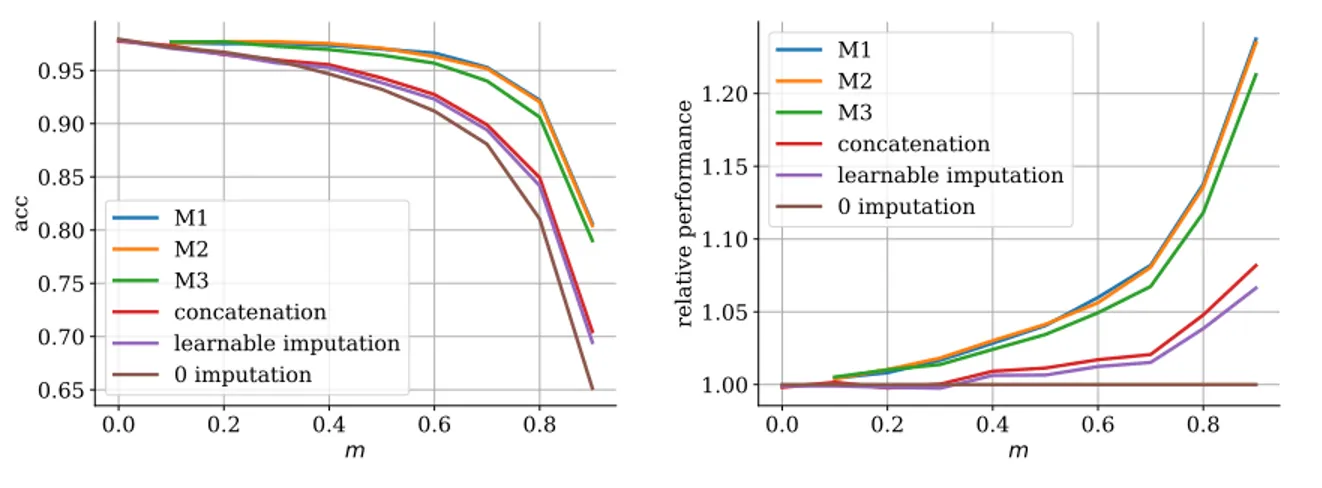
Figure 2. Accuracy for different missing rates m. M1 is the joint generative and discriminative model, trained jointly, M2 is the joint model, with the generative and discriminative models trained separately and M3 is the use of a generative model to impute the missing data to obtain a fully observed dataset, used to train a discriminative model.
p(y|xobs) ≈
K
X
i=1
wkp(y|xobs, xmissk ), (12)
where wk= rk r1+ ... + rK , and rk= p(zk)p(xobs|zk) q(zk|xobs, s) , (13) and (zk, xmissk )k∈{1,...,K} are i.i.d. samples from
p(xmiss|z)q(z|xobs
, s). The prediction (seen as a probability vector) will therefore be a convex combination of the K predictions obtained by imputing the data via autoencoding. Of course, K should be much larger here than during training.
4. Experiments
We apply the different strategies for handling missing data to the dynamically binarized MNIST dataset (LeCun et al.,
1998), over a range of missing rates. The discriminative model is a convolutional neural network with four hidden layers. The generative model is an MLP with two hidden layers of 200 units in the encoder and decoder, and a latent space of dimension 20. During training K = 20 importance samples and a batch size of 100 are used. The generative part of the models is pre-trained for 500k iterations and used as the starting point for M1, M2 and M3.
In M3 the pre-trained model is used immediately to gen-erate single imputations for train, validation and test-sets, using self normalised importance sampling with 10k sam-ples. These are then used to train the discriminative model, do early stopping and get the test-set prediction error. In
M2 the pre-trained generative model is kept fixed while training the discriminative model using the joint loss. In M1 the joint model is trained using the joint loss. In M1 and M2 predictions are done using self-normalized importance sampling on the class probabilities with 10k importance samples, cf. section3.4.2.
Figure2a shows that M1 and M2 perform best and that the performance gap increases with the missing rate. The learning curves in figure2aobscures some of the relative performance gain, so in figure2bthe performance is shown relative to 0-imputation.
The fact that M1 and M2 outperform models that use single imputation indicates that accounting for uncertainty of the missing values is quite valuable.
5. Conclusion and future work
There are many possible approaches to deal with missing data in supervised deep learning. Our small investigations indicate that
• different ways of handling missingness may lead to quite different classification errors,
• accounting for uncertainty of the missing values can be very beneficial, even from a purely predictive per-spective.
While we focused here on a simple convolutional ar-chitecture, it would be interesting to explore other kinds of architectures, from multi-layer perceptrons to recurrent/graph/group-equivariant neural nets.
Acknowledgements
The Danish Innovation Foundation supported this work through Danish Center for Big Data Analytics driven In-novation (DABAI). JF acknowledge funding from the Inde-pendent Research Fund Denmark 9131-00082B.
References
Burda, Y., Grosse, R., and Salakhutdinov, R. Importance weighted autoencoders. In International Conference on Learning Representations, 2016.
Ipsen, N. B., Mattei, P.-A., and Frellsen, J. not-MIWAE: Deep generative modelling with missing not at random data. In review, 2020.
Ivanov, O., Figurnov, M., and Vetrov, D. Variational au-toencoder with arbitrary conditioning. In International Conference on Learning Representations, 2019. Josse, J., Prost, N., Scornet, E., and Varoquaux, G. On the
consistency of supervised learning with missing values. arXiv preprint arXiv:1902.06931, 2019.
Kingma, D. P. and Welling, M. Auto-encoding variational bayes. arXiv preprint arXiv:1312.6114, 2013.
Le Morvan, M., Prost, N., Josse, J., Scornet, E., and Varo-quaux, G. Linear predictor on linearly-generated data with missing values: non consistency and solutions. arXiv preprint arXiv:2002.00658, 2020.
LeCun, Y., Bottou, L., Bengio, Y., and Haffner, P. Gradient-based learning applied to document recognition. Proceed-ings of the IEEE, 86(11):2278–2324, 1998.
Ma, C., Gong, W., Hern´andez-Lobato, J. M., Koenigstein, N., Nowozin, S., and Zhang, C. Partial VAE for hybrid recommender system. In NIPS Workshop on Bayesian Deep Learning, 2018.
Ma, C., Tschiatschek, S., Palla, K., Hernandez-Lobato, J. M., Nowozin, S., and Zhang, C. EDDI: Efficient dy-namic discovery of high-value information with partial VAE. In International Conference on Machine Learning, pp. 4234–4243, 2019.
Mattei, P.-A. and Frellsen, J. Leveraging the exact likelihood of deep latent variable models. In Advances in Neural Information Processing Systems, 2018.
Mattei, P.-A. and Frellsen, J. MIWAE: Deep generative modelling and imputation of incomplete data sets. In International Conference on Machine Learning, pp. 4413– 4423, 2019.
Nazabal, A., Olmos, P. M., Ghahramani, Z., and Valera, I. Handling incomplete heterogeneous data using VAEs. arXiv preprint arXiv:1807.03653, 2018.
Rezende, D. J., Mohamed, S., and Wierstra, D. Stochastic backpropagation and approximate inference in deep gen-erative models. arXiv preprint arXiv:1401.4082, 2014. Rubin, D. B. Inference and missing data. Biometrika, 63(3):
581–592, 1976.
Seaman, S., Galati, J., Jackson, D., and Carlin, J. What is meant by” missing at random”? Statistical Science, pp. 257–268, 2013.
´Smieja, M., Struski, Ł., Tabor, J., Zieli´nski, B., and Spurek, P. Processing of missing data by neural networks. In Advances in Neural Information Processing Systems, pp. 2719–2729, 2018.
Yi, J., Lee, J., Kim, K. J., Hwang, S. J., and Yang, E. Why not to use zero imputation? correcting spar-sity bias in training neural networks. arXiv preprint arXiv:1906.00150, 2019.
Yoon, J., Jordon, J., and Van Der Schaar, M. Gain: Missing data imputation using generative adversarial nets. arXiv preprint arXiv:1806.02920, 2018.