Semiannual and annual variations in the height of the ionospheric F2-peak

HAL Id: hal-00316594

https://hal.archives-ouvertes.fr/hal-00316594

Submitted on 1 Jan 2000

HAL is a multi-disciplinary open access

archive for the deposit and dissemination of sci-entific research documents, whether they are pub-lished or not. The documents may come from teaching and research institutions in France or abroad, or from public or private research centers.

L’archive ouverte pluridisciplinaire HAL, est destinée au dépôt et à la diffusion de documents scientifiques de niveau recherche, publiés ou non, émanant des établissements d’enseignement et de recherche français ou étrangers, des laboratoires publics ou privés.

Semiannual and annual variations in the height of the

ionospheric F2-peak

H. Rishbeth, K. J. F. Sedgemore-Schulthess, T. Ulich

To cite this version:

H. Rishbeth, K. J. F. Sedgemore-Schulthess, T. Ulich. Semiannual and annual variations in the height of the ionospheric F2-peak. Annales Geophysicae, European Geosciences Union, 2000, 18 (3), pp.285-299. �hal-00316594�

Semiannual and annual variations in the height

of the ionospheric F2-peak

H. Rishbeth1_{, K. J. F. Sedgemore-Schulthess}1_{, T. Ulich}2

1_{Department of Physics and Astronomy, University of Southampton, Southampton SO17 1BJ, UK} 2_{SodankylaÈ Geophysical Observatory, TaÈhtelaÈntie 112, SodankylaÈ FIN-90570 Finland}

Received: 12 July 1999 / Revised: 22 November 1999 / Accepted: 3 December 1999

Abstract. Ionosonde data from sixteen stations are used to study the semiannual and annual variations in the height of the ionospheric F2-peak, hmF2. The semiannual variation, which peaks shortly after equi-nox, has an amplitude of about 8 km at an average level of solar activity (10.7 cm ¯ux = 140 units), both at noon and midnight. The annual variation has an amplitude of about 11 km at northern midlatitudes, peaking in early summer; and is larger at southern stations, where it peaks in late summer. Both annual and semiannual amplitudes increase with increasing solar activity by day, but not at night. The semiannual variation in hmF2 is unrelated to the semiannual variation of the peak electron density NmF2, and is not reproduced by the CTIP and TIME-GCM com-putational models of the quiet-day thermosphere and ionosphere. The semiannual variation in hmF2 is approximately ``isobaric'', in that its amplitude corre-sponds quite well to the semiannual variation in the height of ®xed pressure-levels in the thermosphere, as represented by the MSIS empirical model. The annual variation is not ``isobaric''. The annual mean of hmF2 increases with solar 10.7 cm ¯ux, both by night and by day, on average by about 0.45 km/¯ux unit, rather smaller than the corresponding increase of height of constant pressure-levels in the MSIS model. The discrepancy may be due to solar-cycle variations of thermospheric winds. Although geomagnetic activity, which a€ects thermospheric density and temperature and therefore hmF2 also, is greatest at the equinoxes, this seems to account for less than half the semiannual variation of hmF2. The rest may be due to a semiannual variation of tidal and wave energy trans-mitted to the thermosphere from lower levels in the atmosphere.

Key words: Atmospheric composition and structure (thermosphere ± composition and chemistry) ± Ionosphere (mid-latitude ionosphere)

1 Introduction

Several atmospheric, ionospheric and geomagnetic pa-rameters display a regular semiannual (6-monthly) variation, with maxima near the March and September equinoxes. They include the peak electron density of the ionospheric F2-layer (NmF2) in some parts of the world (Burkard, 1951; Yonezawa and Arima, 1959; Chaman Lal, 1992); the height of the F2-layer peak (hmF2) (Becker, 1967); the neutral air density q in the thermo-sphere (Paetzold and ZschoÈrner, 1961); and geomagnetic indices such as Kp and Ap (Bartels, 1963; Green, 1984). Semiannual oscillations also exist in the lower and middle atmosphere. Annual (12-monthly) variations also exist in hmF2 and q, with maxima usually in summer. The case of noon NmF2 is complicated: in some parts of the world its predominant variation is semiannual, but elsewhere it is annual, usually with a winter maximum (e.g. Yonezawa and Arima, 1959; Yonezawa, 1971; Torr and Torr, 1973).

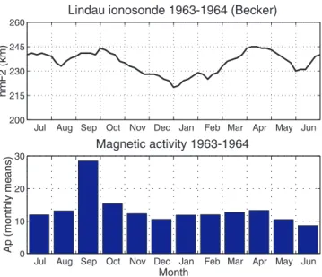
Most of these annual and semiannual phenomena have been extensively studied. An exception is the semiannual variation in hmF2, which does not seem to have received much discussion since Becker's (1964, 1967) papers thirty years ago. Figure 1 shows the 27-day running mean of noon hmF2 for a twelve month period in 1963±1964 at Lindau, Germany, derived by real height N(h) analysis of ionograms by Becker (1967). The day-to-day variability of hmF2 has been considerably smoothed by the 27-day averaging (judging from Bec-ker's daily values during this period which are shown in Fig. 5 of Rawer, 1969). Also plotted in Fig. 1 is the average month-by-month variation of the magnetic parameter Ap, which shows the equinox peaks in mag-netic activity, the in¯uence of which is discussed in Sect. 4.2 (the September peak is in¯uenced by an immense storm, with Ap = 126 on 22 September, 1963). During

these 12 months, the solar 10.7 cm radio ¯ux F10.7(used

as a conventional indicator of solar activity) was fairly steady, in the range 75±90 ¯ux units, except in late

September 1963 when it rose to around 100 units. The semiannual variation is not so consistent or well-de®ned

for the period 1957±1958. The dependence on F10.7 of

day-to-day values of hmF2 is not clear-cut, in that the Lindau data for 1958 show a great deal of scatter when

plotted against F10.7 (Becker, 1964). Eccles et al. (1967)

commented on Becker's results, but they could only reproduce a semiannual variation of hmF2 by the device of imposing a semiannual temperature variation in their model.

Further investigation of hmF2 is required. Concen-trating on midday and midnight, we tackle the question in two ways: in Sect. 2 by Fourier analysis of hmF2 data from several ionosonde stations over three solar cycles, and in Sect. 3 by using the global thermospheric models TIME-GCM (Roble et al., 1988) and CTIP (Fuller-Rowell et al., 1996; Millward et al., 1996a). In Sect. 4 we investigate whether the variations of hmF2 are ``iso-baric'', by comparing them with the variations in height of ®xed pressure-levels in the thermosphere, as expressed by the MSISE-90 thermospheric model. We also estimate the e€ect on hmF2 of geomagnetic activity, in particular the equinoctial peaks in Ap. In Sect. 5 we review possible causes of the semiannual variation of hmF2.

2 Values of hmF2 derived from ionosonde data 2.1 Analysis

Our data comprise values of hmF2 for sixteen stations (Table 1a, b). The values of hmF2 were derived from ``MUF factors'' (M3000) tabulated in ionosonde data taken from the National Geophysical Data Centre Vertical Sounding Database, using the formulae pro-posed by Shimazaki (1955) and Bilitza et al. (1979). M3000 is the factor which, in theory, relates the

maximum usable frequency for propagation over a 3000 km path to the ordinary critical frequency foF2. According to the ``Shimazaki formula'', which assumes the idealized case of radio waves re¯ected from a parabolic F2 layer above a spherical Earth:

hmF2 ˆ f1490=M3000g ÿ 176 ‰kmŠ …1a†

The ``Bilitza formula'', which allows for the e€ect of ionization below the F2-layer, takes the form

hmF2 ˆ f1490=…M3000 ‡ DM…X ††g ÿ 176 ‰kmŠ …1b†

where DM(X) is an empirical function of the critical frequency ratio X = foF2/foE, taking account of sunspot number and geomagnetic latitude. The correc-tion is important by day, as we show later, but is suciently small at night for the plain ``Shimazaki formula'' Eq. (1a) to be used. The formulas are unreliable if M3000 is small, i.e. the layer is high, or if foF2 is too close to foE (e.g. Dudeney, 1983). Ulich and Turunen (1997) ®nd that the Bilitza formula overesti-mates daytime hmF2, on average by 18 km, as com-pared to the value found from real height inversion (using the polynomial method of Titheridge, 1969). As the error depends on X and increases when X is large (McNamara et al., 1987), as at solar maximum, it may a€ect our results for the solar cycle variations of hmF2. It is most desirable to use data that are consistently scaled and well-calibrated across any changes of instru-ment and site. Several stations that we used meet this criterion, but not necessarily for the whole period 1957± 1994 spanned by our data. To increase con®dence in the analysis, we imposed the conditions M3000 > 2.5 and X > 1.7, which limited the number of stations for which we had MUF data of acceptable quality, especially at night. Only a few stations in the Southern Hemisphere met the criteria, and we omitted stations near the magnetic equator, because of doubts about the reliabil-ity of any MUF-based formula. We use monthly medians, averaging the daytime values of hmF2 over the period 10±14 LT and the nighttime values over 22± 02 LT. Our analysis program makes a linear interpola-tion through data gaps of up to three months while rejecting data containing longer gaps; for most stations, we have useful results for 25±30 years. As magnetic activity is enhanced at the equinoxes, the median values for equinox months correspond to higher levels of Ap than do those for solstice months; in Sect. 4.2 we discuss the possible e€ect of this on our results.

2.2 Annual means of hmF2

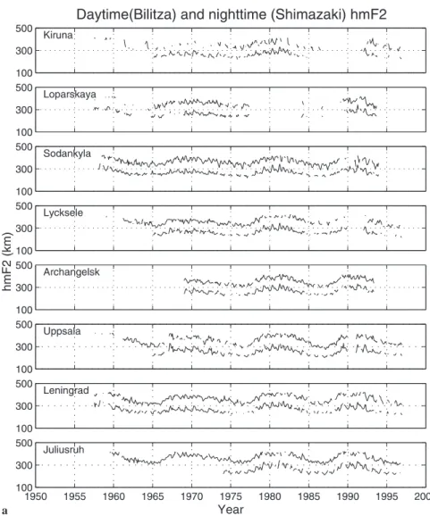
The month-by-month data for sixteen stations are shown in Fig. 2. At all these stations, hmF2 is clearly higher at night than by day, and the day and night plots clash only at Kerguelen. Perusal of the plots shows an overlying solar-cycle variation everywhere, with marked station-to-station di€erences in annual and semiannual variations. For example, by day the annual variations are especially strong at Port Stanley, and at Moscow the semiannual variation has noticeably higher peaks in

Fig. 1. Plot of hmF2 at Lindau (52°N), as derived from ionograms by Becker (1967), and the geomagnetic index Ap for the 12-month period July 1963 to June 1964

spring than in autumn. Table 1a, b gives values of the

annual mean h0 for F10.7 = 140, which represents a

midway value between solar minimum (F10.7» 70) and

the peak values of F10.7at the three solar maxima (232

in 1958, 156 in 1970, 203 in 1981 and 212 in 1989); 140 is

also the value of F10.7 used in the TIME-GCM runs

(Sect. 3.1). The stations are arranged in order of decreasing magnetic latitude though, apart from Mos-cow and Port Stanley, the order would be unchanged if instead they were arranged geographically. The values

of h0 for the Northern Hemisphere stations are rather

uniform, averaging 268 km by day and 369 km at night, with no clear latitude trend. The southern stations are less consistent, but on average hmF2 is higher by day (279 km) and lower at night (351 km) than in the Northern Hemisphere. The rate of increase with solar

¯ux, dh0/dF10.7 (shown for a representative selection of

stations), averages 0.44±0.46 km/unit by day and night in both hemispheres. As mentioned in Sect. 2.1, the

values of dh0/dF10.7 may be a little too large, the

overestimate being perhaps 0.05 km/unit. 2.3 Fourier analysis to derive annual and semiannual components

For the Fourier analysis, we take twelve monthly data values for a given year and ®t mean, annual and semiannual components, thus:

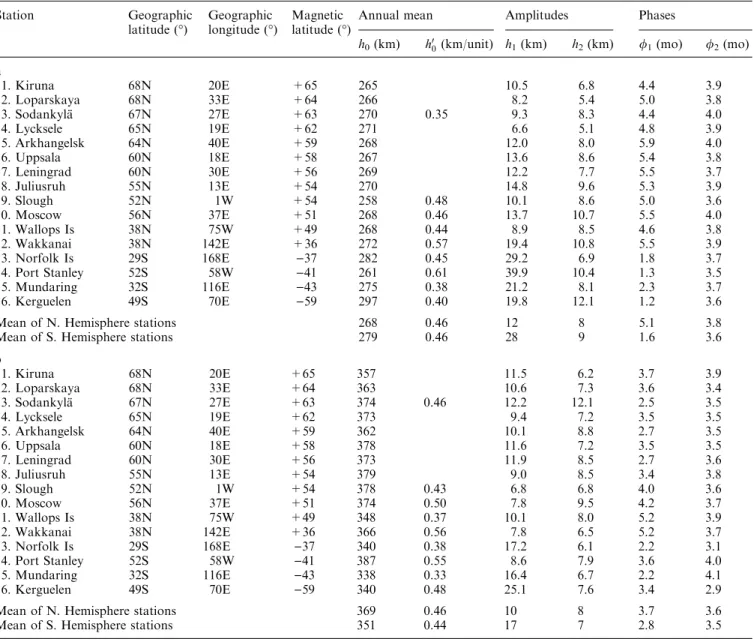
hmF2 ˆ h0‡ h1cos……p=6†…t ÿ /1†† ‡ h2cos……p=3†…t ÿ /2†† …2† b 1. Kiruna 68N 20E +65 357 11.5 6.2 3.7 3.9 2. Loparskaya 68N 33E +64 363 10.6 7.3 3.6 3.4 3. SodankylaÈ 67N 27E +63 374 0.46 12.2 12.1 2.5 3.5 4. Lycksele 65N 19E +62 373 9.4 7.2 3.5 3.5 5. Arkhangelsk 64N 40E +59 362 10.1 8.8 2.7 3.5 6. Uppsala 60N 18E +58 378 11.6 7.2 3.5 3.5 7. Leningrad 60N 30E +56 373 11.9 8.5 2.7 3.6 8. Juliusruh 55N 13E +54 379 9.0 8.5 3.4 3.8 9. Slough 52N 1W +54 378 0.43 6.8 6.8 4.0 3.6 10. Moscow 56N 37E +51 374 0.50 7.8 9.5 4.2 3.7 11. Wallops Is 38N 75W +49 348 0.37 10.1 8.0 5.2 3.9 12. Wakkanai 38N 142E +36 366 0.56 7.8 6.5 5.2 3.7 13. Norfolk Is 29S 168E )37 340 0.38 17.2 6.1 2.2 3.1 14. Port Stanley 52S 58W )41 387 0.55 8.6 7.9 3.6 4.0 15. Mundaring 32S 116E )43 338 0.33 16.4 6.7 2.2 4.1 16. Kerguelen 49S 70E )59 340 0.48 25.1 7.6 3.4 2.9

Mean of N. Hemisphere stations 369 0.46 10 8 3.7 3.6

Mean of S. Hemisphere stations 351 0.44 17 7 2.8 3.5

Table 1. a Height hmF2 at midday (10±14 LT) for solar ¯ux F10.7

= 140 units, computed from ionosonde ``MUF'' data; h0is the

annual mean, h0

0is the rate of change dh0/dF10.7; the amplitudes h1

and h2refer to the annual and semiannual components as de®ned

in Eq. (2). Stations are arranged in order of magnetic invariant latitude. b. Height hmF2 at night (22-02 LT) for solar ¯ux F10.7=

140 units, computed from ionosonde ``MUF'' data. Layout as for Table 1a

Station Geographic

latitude (°) Geographiclongitude (°) Magneticlatitude (°) Annual mean Amplitudes Phases

h0(km) h00(km/unit) h1(km) h2(km) /1(mo) /2(mo)

a 1. Kiruna 68N 20E +65 265 10.5 6.8 4.4 3.9 2. Loparskaya 68N 33E +64 266 8.2 5.4 5.0 3.8 3. SodankylaÈ 67N 27E +63 270 0.35 9.3 8.3 4.4 4.0 4. Lycksele 65N 19E +62 271 6.6 5.1 4.8 3.9 5. Arkhangelsk 64N 40E +59 268 12.0 8.0 5.9 4.0 6. Uppsala 60N 18E +58 267 13.6 8.6 5.4 3.8 7. Leningrad 60N 30E +56 269 12.2 7.7 5.5 3.7 8. Juliusruh 55N 13E +54 270 14.8 9.6 5.3 3.9 9. Slough 52N 1W +54 258 0.48 10.1 8.6 5.0 3.6 10. Moscow 56N 37E +51 268 0.46 13.7 10.7 5.5 4.0 11. Wallops Is 38N 75W +49 268 0.44 8.9 8.5 4.6 3.8 12. Wakkanai 38N 142E +36 272 0.57 19.4 10.8 5.5 3.9 13. Norfolk Is 29S 168E )37 282 0.45 29.2 6.9 1.8 3.7 14. Port Stanley 52S 58W )41 261 0.61 39.9 10.4 1.3 3.5 15. Mundaring 32S 116E )43 275 0.38 21.2 8.1 2.3 3.7 16. Kerguelen 49S 70E )59 297 0.40 19.8 12.1 1.2 3.6

Mean of N. Hemisphere stations 268 0.46 12 8 5.1 3.8

where the amplitudes h0, h1, h2 are in kilometres, and

time t and the phases /1 and /2 are in months, zero

phase being a maximum in mid-December. These phases, based on one-monthly data points, should be accurate to ‰ month or possibly slightly better.

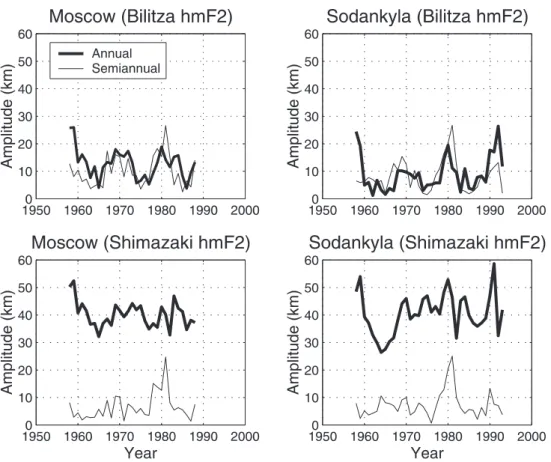
Figure 3 shows the importance of the ``M3000 correction'' DM for underlying ionization, using two stations with very good datasets, Moscow and Sod-ankylaÈ. The upper boxes show the annual and

semian-nual amplitudes h1and h2for daytime, derived by using

the ``Bilitza formula'', Eq. (1b), which includes the correction; the lower boxes show the corresponding results given by the plain ``Shimazaki formula'', Eq. (1a), which does not. Applying the correction DM clearly makes a great di€erence to the annual amplitudes, but has much less e€ect on the semiannual amplitudes.

The reason is not far to seek. If DM is omitted or is incorrect, the computed annual component in hmF2 is strongly in¯uenced by the F1-layer, which is most prominent in summer and usually absent in winter, as well as by the E-layer. As the critical frequencies foE and foF1 are closely controlled by the solar zenith angle, which is the same at both equinoxes, variations of the E- and F1-layers should not seriously a€ect the semi-annual component.

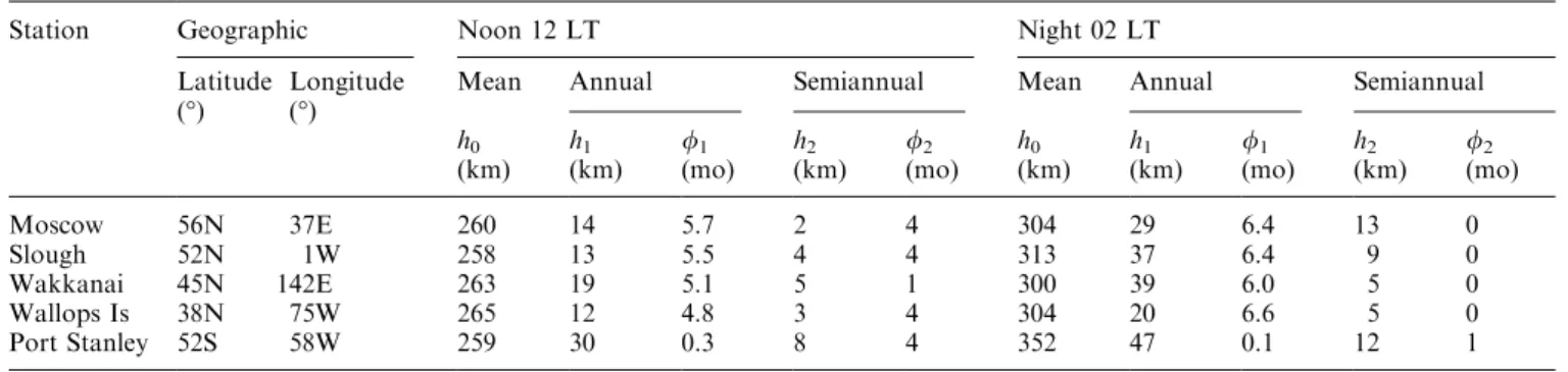
Figure 4 shows periodograms for ®ve of the stations, chosen to give a wide geographical spread. It is obvious that the relative strength of the annual and semiannual components may be quite di€erent between day and night at one station, and also that it varies greatly between stations. Compare, for example, the almost pure annual variation at Port Stanley (day) to the predominantly semiannual variation at Moscow (night). With a data run of 30 years, as available at most of these stations, the resolution is of order 3% (or 0.4 month) for the annual variation and 1.5% (or 0.1 month) for the semiannual variation. Tests made for SodankylaÈ, using the polynomial method of Titheridge (1969) to compute real heights, give similar results but with a rather smaller semiannual/annual ratio than shown in Fig. 3.

2.4 Annual and semiannual components: results

Figure 5a for day and 5b for night show the amplitudes

h0, h1, h2plotted against the annual mean values of F10.7

for the same ®ve stations as used in Fig. 4, each point representing an individual year. The data points are well ®tted by straight lines, with high correlation coecients

r(h0), both by day (0.81±0.94) and at night (0.75±0.92).

Fig. 2a, b. Time sequences of day (10±14 LT) (lower curve in each box) and night (22±02 LT) (upper curve in each box) values of hmF2, computed from tabulated MUF factors derived from ionograms, using monthly values for 16 stations arranged in order of decreasing magnetic latitude. a Kiruna to Juliusruh; b Slough to Kerguelen

The 5% signi®cance levels (2 standard deviations) are in most cases (‹) 20±30 km.

The centre and right-hand boxes in Fig. 5a, b show

the plots of h1 and h2 versus F10.7, also ®tted with

straight lines. These plots contain a great deal of scatter, but by day there is a clear upward trend. For northern

stations the correlation coecients r(h1) are in the range

0.35±0.8 and r(h2) are in the range 0.4±0.7, but the

correlation coecients are on the whole smaller at southern stations (0.07±0.5). The rates of increase are

such that, from solar minimum (F10.7= 70) to solar

maximum (F10.7 = 200), daytime h1 increases on

average by 10 km and daytime h2 by 8 km. At night

the variations of h1and h2with F10.7are not signi®cant;

the correlation coecients are small (mostly <0.3) and most are negative, implying a slight tendency for the

amplitudes to decrease with increasing F10.7. Numerical

values of h0, h1, h2at F10.7= 140 for all sixteen stations

are given in Table 1a for day and 1b for night.

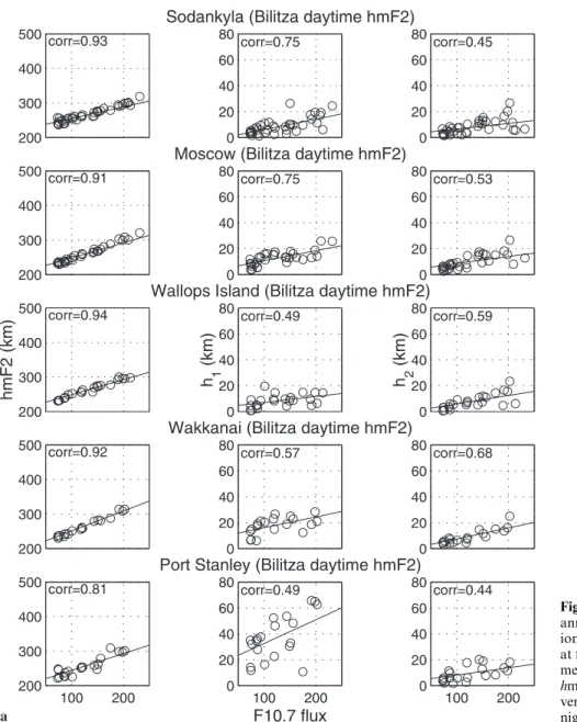
Port Stanley stands out from the other stations

because of its very large day-to-night change in h0 and

its large daytime annual component h1, which doubles in

amplitude from solar minimum (30 km) to solar

max-imum (60 km). The low daytime h0, high nighttime h0,

and large daytime amplitude h1 at Port Stanley is seen

also at number 14 in Fig. 6, which shows the Fourier results for all stations. A large daytime annual

compo-nent h1is seen at the southern stations (13±16), and at

Wakkanai in the Northern Hemisphere (12). Other

notable features are the low daytime h0at Slough (9) and

the low nighttime h0at Wallops Island (11).

As for phases, Table 1a shows that, at northern

stations by day, the annual phase /1is in the range 4±6

months, corresponding to maximum in mid-April to mid-June, and in late summer (1±2 months) at the

southern stations (13±16). The semiannual phase /2 is

consistently near equinox (3±4 months). At night, Table 1b shows that the semiannual variation again has its maxima near equinox, but the annual phase is usually earlier than by day, the maximum being at 2±5 months (February±May). We found no well-de®ned

variation of the phases with F10.7though, at lower F10.7,

when the amplitudes are smaller and the phases are less well determined, there is more scatter, particularly in the annual component.

From the midlatitude results, in particular the

con-sistent values of /2, we conclude that the semiannual

variation of noon hmF2 is real. Its amplitude h2is rather

smaller than the annual amplitude h1. The combination

of the semiannual spring maximum and the early summer

maximum of the annual component produces an April or May maximum of noon hmF2 at northern stations; in the south, with a relatively small semiannual component, the maximum occurs in January or February.

2.5 Incoherent scatter data on hmF2 at Millstone Hill We examined daytime values of hmF2 obtained in 1968± 1971 from the incoherent scatter radar at Millstone Hill (43°N), given by Papagiannis et al. (1975) in the following form:

hmF2 ˆ 280 ‡ 9Kp ˆ 304 ‰kmŠ …summer† …3a†

hmF2 ˆ 290 ‡ 4Kp ˆ 301 ‰kmŠ …equinox† …3b†

hmF2 ˆ 265 ‡ 5Kp ˆ 278 ‰kmŠ …winter† …3c†

where the last value in each line is for Kp = 2.7, the mean value for the years in question. In this period the average

F10.7is 144, so these values of hmF2 may reasonably be

compared with the ionogram-derived values for F10.7=

140. Annual and semiannual amplitudes and phases cannot be determined from three values, but we can derive minimum amplitudes by assuming that the annual component maximizes in summer and the semiannual component at equinox. With these assumptions, the annual mean is 296 km, the annual amplitude is 13 km and the semiannual amplitude is 10 km, all of which are rather greater than the values derived from ionosonde data at northern stations (Table 1a). If the phases are not as assumed, the amplitudes will be greater.

3 Modelling of hmF2 with global thermosphere-ionosphere models

3.1 Global modelling using TIME-GCM

In Table 2 we show results obtained from the TIME-GCM Community Climate Model 3 for seven stations (which were chosen for another investigation, ®ve of them being the same used in our data analysis); the values of hmF2 were kindly made available by R. G. Roble. For the simulation, solar activity is ®xed at a moderate level

(F10.7 = 140 ¯ux units) and magnetic conditions are

quiet. We took smoothed daily values of hmF2 to represent day 16 of each month; the daytime results are for 12 LT, the nighttime results for 02 LT (which, for our purposes, does not di€er signi®cantly from midnight).

Table 2 shows that hmF2 is consistently higher in summer than in winter, both by day and by night. By

day, the amplitude h1is larger in the Southern than in the

Northern Hemisphere, but not necessarily at night. In all cases the annual maximum occurs in local summer. The semiannual variation is barely signi®cant, the amplitude

h2being small compared to h1at all the stations, so the

semiannual phase is poorly determined. As TIME-GCM uses a height step of ‰ scale height, corresponding to about 25 km, the ®tting procedure used to derive hmF2 should be accurate to one-third of a height step, and thus

better than 10 km, so the values of h1should be reliable

even if those of h2are not. No relationship is found in

the TIME-GCM results between the amplitudes of the semiannual variations of hmF2 and those of NmF2.

Fig. 3. Comparison of the am-plitudes of the annual and semi-annual components of hmF2, with (``Bilitza'') and without (``Shimazaki'') corrections for ionization underlying the F2-layer for day (10±14 LT)

3.2 Global modelling using CTIP

The CTIP model was run as described by Zou et al. (2000), for each month of the year, assuming constant

solar activity of F10.7= 100 units and quiet geomagnetic

conditions (Kp = 2, Ap = 7). At noon, the mean level

h0 is about 260 km at high midlatitudes but, below

magnetic latitudes ‹25°, h0increases towards a value of

about 360 km at the magnetic equator. With a compu-tational height step of one scale height (typically 45 km),

Fig. 4. Day (10±14 LT) and night (22±02 LT) periodograms of hmF2 for ®ve stations Table 2. Midday and night hmF2: amplitudes and phases from TIME-GCM model, F10.7= 140

Station Geographic Noon 12 LT Night 02 LT

Latitude

(°) Longitude(°) Mean Annual Semiannual Mean Annual Semiannual

h0 h1 /1 h2 /2 h0 h1 /1 h2 /2

(km) (km) (mo) (km) (mo) (km) (km) (mo) (km) (mo)

Moscow 56N 37E 260 14 5.7 2 4 304 29 6.4 13 0

Slough 52N 1W 258 13 5.5 4 4 313 37 6.4 9 0

Wakkanai 45N 142E 263 19 5.1 5 1 300 39 6.0 5 0

Wallops Is 38N 75W 265 12 4.8 3 4 304 20 6.6 5 0

the accuracy of hmF2 is probably one-third of this, about 15 km, so the amplitudes are not very accurately de®ned. The phases are accurate to within 1 month.

Omitting the equatorial zone within magnetic lati-tudes ‹25°, the Fourier components may be

summa-rized as follows. At noon, the annual amplitude h1 is

about 15 km at northern midlatitudes. In the Southern

Hemisphere h1varies with longitude, being about 15 km

in western longitudes and 20±25 km in eastern

longi-tudes. The phase /1 corresponds closely to summer

solstice, i.e. 0±1 month in the southern magnetic hemi-sphere, 6 months in the north, the boundary being at the magnetic and not the geographic equator. The

semian-nual amplitude h2is very small (<5 km) at midlatitudes,

with phase /2» 3 corresponding to equinox. The results

for midnight are broadly similar, except that the mean level is 310±360 km (varying with longitude); the semi-annual component is slightly larger than by day, with

h2£ 10 km and maxima near solstice (/2» 0). The CTIP

results for higher solar activity, F10.7 = 180, show a

similar distribution of annual and semiannual

compo-nents, but with an amplitude ratio h1/h2 that is rather

smaller (typically by about 30%) than at F10.7= 100.

Comparing the CTIP and TIME-GCM results for the seven stations listed in Table 2, we ®nd a great deal of similarity. Averaged over the seven stations, the mean

values h0 are about 5 km lower for CTIP than for

TIME-GCM but about 12 km higher at night. The

annual amplitude h1is in most cases smaller for CTIP

than for TIME-GCM, notably at Port Stanley. The di€erences seem to be associated with the meridional winds, which are particularly strong in TIME-GCM in this sector, and are very dependent on the details of the neutral temperature and pressure distributions. The phase of the annual component of hmF2, with maxi-mum in summer in both models, agrees with all the noon data and almost all the night data shown in Table 1a, b. In both CTIP and TIME-GCM, most of the

semi-annual amplitudes h2are only a few kilometres which,

being rather small compared with the corresponding h1,

Fig. 5. a Annual means, annual and semi-annual ampitudes of hmF2, derived from ionograms, plotted versus 10.7 cm solar ¯ux at ®ve stations for day (10±14 LT). b Annual means, annual and semiannual ampitudes hmF2, derived from ionograms, plotted versus 10.7 cm solar ¯ux at ®ve stations for night (22±02 LT)

are not well determined by the analysis, nor are the

derived phases /2 trustworthy. The important

conclu-sions are that the CTIP and TIME-GCM results for hmF2 agree quite well, and that the semiannual com-ponents are much smaller than are found in the ionosonde data.

4 Semiannual variations in MSIS

According to Rishbeth and Edwards (1989), the F2-peak at a given local time should lie approximately at a constant pressure-level, for all seasons and all levels of solar activity. For midlatitude stations generally, these ®xed pressure-levels are 20 lPa at noon and 2 lPa at midnight. We can test this assertion against the well-known MSIS (Mass Spectrometer/Incoherent Scatter) model, which is widely used to represent the behaviour of thermospheric parameters. To do this, we examine

how the heights hPD and hPN of the daytime and

nighttime levels, de®ned by the pressure values just quoted, vary with season and solar activity, and compare them with the ionosonde values of hmF2. For this purpose we use the extended version MSISE-90 of Hedin (1991), although, since we consider only F-region heights between about 200 and 450 km, the extension below 90 km is not relevant to our study and for simplicity we use the term MSIS. As the nighttime TIME-GCM data used in Sect. 3.1 are for 02 LT instead of 00 LT (midnight), we use 02 LT for the MSIS study, which should make no signi®cant di€erence.

4.1 Quiet-day MSIS data

We ran the MSIS model for the stations shown in Figs. 4 and 5, namely SodankylaÈ, Slough, Wakkanai, Wallops Island and Port Stanley. As the MSIS parameters vary

only slowly with latitude and longitude, the choice of locations is not critical, and it seemed unnecessary to do the calculations for all sixteen stations. We use the same two local times, 12 LT and 02 LT, and three levels of

solar activity, F10.7= 70, 140 and 200. To test the e€ect

of geomagnetic activity, we use two di€erent conditions: ``quiet'', for which we take Ap = 3; and ``average'', for which we take Ap = 13, 17 and 20 to represent average

conditions for the three levels of F10.7. We further

discuss the e€ect of varying Ap in Sect. 4.2.

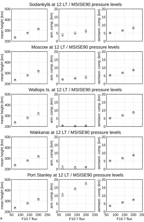
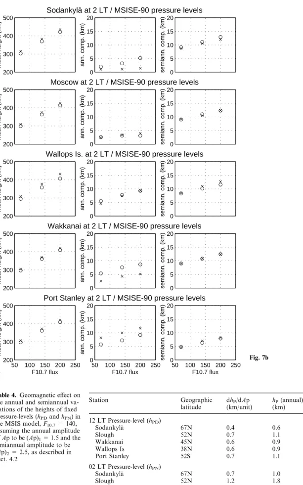
In Fig. 7a for day and 7b for night, the MSIS

pressure-level heights hPD and hPN are plotted against

F10.7, with circles denoting quiet and crosses denoting

average magnetic conditions. Some numerical data are

shown in Table 3. The annual mean values of hPD and

hPN (tabulated for F10.7 = 140) agree quite well with

hmF2 (Table 1a, b). They do not vary much between stations, and neither do their rates of change with solar

activity, which are dhPD/dF10.7» 0.6 km/unit and dhPN/

dF10.7» 0.9 km/unit (averaged over the range F10.7= 70

to 200).There is some di€erence between day and night

in that, as F10.7increases, the slope dhPD/dF10.7increases

slightly while dhPN/dF10.7decreases, but these tendencies

are too small to be easily seen in Fig. 7a, b.

The mean temperatures T at these pressure-levels, also shown in Table 3, vary from place to place, though not in the same way as the pressure-level heights, which depend on composition as well as on temperature. The mean rates of increase of temperature

with F10.7 are similar at all stations, about 3.7 K/unit

for day and 2.9 K/unit for night, both decreasing with

increasing F10.7.

The phases of the semiannual variations of hPD and

hPN are very consistent, namely 3.9 months, which

corresponds to a maximum about 1 month after equinox. By day, the maximum of the annual compo-nent occurs near summer solstice, the phases being 6.0 months at the northern stations and 0.3 month at Port Stanley, though at night the annual phases are not consistent between stations.

The semiannual variations in MSIS agree very well in phase, and broadly agree in amplitude, with those derived from the ionosonde data (Table 1a, b). The annual variations disagree: in particular, the remarkably small daytime amplitudes at Wallops Island and Wak-kanai have no counterpart in the ionosonde data (Table 1a) nor in the TIME-GCM simulations (Table 2). The nighttime MSIS amplitude at SodankylaÈ

Fig. 6. Day and night values of annual mean hmF2 (h0) and the amplitude and

phase of the annual component (h1, /1) and

semiannual component (h2, /2) for day (10±

14 LT) and night (22±02 LT), solar 10.7 ¯ux 140 units. The stations are arranged in north-to-south order of magnetic latitude (1, Kiruna, 2, Loparskaya, 3, SodankylaÈ, 4, Lycksele, 5, Arkhangelsk, 6, Uppsala, 7, Leningrad, 8, Juliusruh, 9, Slough, 10, Moscow, 11, Wallops Is, 12, Wakkanai, 13, Norfolk Is, 14, Port Stanley, 15, Mun-daring, 16, Kerguelen)

is also small. Another obvious discrepancy is that the

MSIS heights hPD and hPN increase more rapidly with

increasing F10.7than do the F2-layer mean heights h0.

4.2 How geomagnetic activity a€ects the annual and semiannual variations of pressure-levels

We now discuss the e€ect of geomagnetic activity, which peaks at the equinoxes (Fig. 1). Magnetic activity increases thermosphere temperature and density, so it raises the heights of ®xed pressure-levels. Thus the seasonal variations of magnetic activity a€ect the annual and semiannual variations of hmF2. We cannot directly investigate this e€ect in our ionosonde data, because that would entail separating ``quiet'' and ``disturbed'' days, which would seriously reduce the quantity of usable hmF2 data. Nor do the TIME-GCM and CTIP simulations described in Sect. 3 shed any light on the matter, because they assume quiet conditions with low Ap. We can, however, estimate the ``geomagnetic

e€ect'', i.e. how much the ®xed pressure-levels hPD and

hPN are raised when average levels of magnetic activity

are put into the MSIS model.

For this purpose we use monthly mean values of Ap derived by M. Mendillo and colleagues (private com-munication, 1998) from geomagnetic data for 1955± 1995, extracted from the CD-ROM produced by World Data Centre A for Solar-Terrestrial Physics. Three groups of years were de®ned according to the annual

mean values of F10.7, namely low (F10.7< 80), medium

(140 < F10.7< 155) and high (F10.7> 175), with mean

values of Ap for ``quiet'' and ``average'' conditions as mentioned in Sect. 4.1. These groups correspond well

to the levels F10.7 = 70, 140, 200 used for the MSIS

runs.

We ran MSIS with the ``average'' values of Ap, and

compared the heights hPDand hPNwith those obtained

from the ``quiet'' runs (Ap = 3). This enabled us to

obtain the rates of change dhPD/dAp for day (0.4±

0.7 km/unit), and dhPN/dAp for night (0.7±1.3 km/unit),

as shown in Table 4. We now apply these results to annual and semiannual variations, making the

simpli-fying assumption that hPD and hPN vary linearly with

Ap, which seems reasonable for the moderate values of Ap involved. On average the temperature is 45 K higher at noon, and 63 K higher at night, for the ``average'' values of Ap than for the ``quiet'' values.

For ``medium'' solar activity (F10.7 = 140), the

semiannual variation of Ap has amplitude (Ap)2= 2.5

units and phase 4 months (maximum 1 month after equinox). The annual variation is smaller, with

ampli-tude (Ap)1= 1.5 units and phase also about 4 months.

Because of its phase, the annual component of Ap is small at the solstices, its e€ect being to increase Ap at the March equinox and reduce it at the September

equinox. (The amplitudes vary somewhat with F10.7, and

so does the annual phase; but we need not go into those details for our rough estimate of the geomagnetic e€ect.)

Combining the values of dhPD/dAp and dhPN/dAp

with the amplitudes (Ap)1 and (Ap)2, we estimate the

amplitude of the annual oscillations in hPD and hPN as

shown in Table 4. The geomagnetic e€ect in the semiannual component is seen to be quite small, only 1±1.5 km by day and 2±3 km at night, and even smaller in the annual component. Comparing these with the

semiannual amplitudes h2 shown in Table 1, we

con-clude that the equinoctial peaks in geomagnetic activity

Station Geographic

latitude Annual mean Amplitude dh(200-70) (km/unit)P/dF10.7

T (K) hP(km) h1(km) h2(km) 20 lPa at 12 LT (hPD) (F10.7= 140, Ap = 3) SodankylaÈ 67N 1005 274 5 7 0.61 Slough 52N 1036 277 4 7 0.64 Wakkanai 45N 1058 278 1 7 0.63 Wallops Is 38N 1062 277 0.2 7 0.67 Port Stanley 52S 1020 276 14 6 0.62 Di€erences F10.7: (140-70) 284 42 ± 1.8 F10.7: (200-140) 200 38 ± 1.7 2 lPa at 02LT (hPN) (F10.7= 140, Ap = 3) SodankylaÈ 67N 938 370 3 11 0.92 Slough 52N 919 364 6 11 0.90 Wakkanai 45N 878 361 8 11 0.88 Wallops Is 38N 916 358 8 10 0.94 Port Stanley 52S 865 362 7 6 0.88 Di€erences F10.7: (140-70) 231 64 ± 1.8 F10.7: (200-140) 148 50 ± 1.6

Table 3. Temperatures (T), and the heights (hP) and annual and

semiannual variations of ®xed pressure-levels derived from MSISE-90. The two bottom lines in each part of the Table show

the variations with F10.7 (not shown for the annual component

because they vary considerably between stations). See text regarding phases

cause only a minor part of the semiannual variation in hmF2. A similar conclusion may be drawn from the Millstone Hill data of Papagiannis et al. (1975) dis-cussed in Sect. 2.5.

5 Discussion

The ionosonde data show that the semiannual variation in hmF2 is real. Its phase is consistent, with maxima shortly after equinox, and its amplitude increases with

increasing F10.7. At high F10.7 the semiannual

compo-nent is roughly equal to the annual compocompo-nent, which is fairly constant in phase (maximum in summer,

mini-mum in winter), becoming earlier with increasing F10.7.

The combination of the annual and semiannual com-ponents generally leads to a maximum of hmF2 in April or May in the north, and January or February in the south.

The southern stations (Port Stanley, particularly) and also Wakkanai show strong annual variations of hmF2 by day, which may be attributed to the seasonal variations of meridional winds. Wind e€ects are partic-ularly strong at Port Stanley and Wakkanai, which are situated in longitudes remote from the magnetic poles (Rishbeth, 1998). At Port Stanley, the e€ect of strong

diurnally varying winds is seen in the annual mean h0;

the night value of 387 km is the highest, and the day value of 261 km the second lowest, of any of the 16 stations. Furthermore, the magnetic dip angle I is close

200 300 400 500 mean height (km) 0 5 10 15 20

Sodankylä at 12 LT / MSISE90 pressure levels

ann. comp . (km) 0 5 10 15 20 semiann. comp . (km) 200 300 400 500 mean height (km) 0 5 10 15 20

Moscow at 12 LT / MSISE90 pressure levels

ann. comp . (km) 0 5 10 15 20 semiann. comp . (km) 200 300 400 500 mean height (km) 0 5 10 15 20

Wallops Is. at 12 LT / MSISE90 pressure levels

ann. comp . (km) 0 5 10 15 20 semiann. comp . (km) 200 300 400 500 mean height (km) 0 5 10 15 20

Wakkanai at 12 LT / MSISE90 pressure levels

ann. comp . (km) 0 5 10 15 20 semiann. comp . (km) 50 100 150 200 250 200 300 400 500 mean height (km) F10.7 flux 50 100 150 200 250 0 5 10 15 20

Port Stanley at 12 LT / MSISE90 pressure levels

ann. comp . (km) F10.7 flux 50 100 150 200 250 0 5 10 15 20 semiann. comp . (km) F10.7 flux a

Fig. 7. a Annual means, annual and semi-annual amplitudes of the ®xed pressure-level 20 lPa (approximately corresponding to daytime hmF2) plotted versus 10.7 cm solar ¯ux at ®ve stations for noon (12 LT). b Annual means, annual and semiannual amplitudes of the ®xed pressure-level 2 lPa (approximately corresponding to nighttime hmF2) plotted versus 10.7 cm solar ¯ux at ®ve stations for night (02 LT)

200 300 400 500 mean height (km) 0 5 10 15 20

Sodankylä at 2 LT / MSISE-90 pressure levels

ann. comp. (km) 0 5 10 15 20 semiann. comp. (km) 200 300 400 500 mean height (km) 0 5 10 15 20

Moscow at 2 LT / MSISE-90 pressure levels

ann. comp. (km) 0 5 10 15 20 semiann. comp. (km) 200 300 400 500 mean height (km) 0 5 10 15 20

Wallops Is. at 2 LT / MSISE-90 pressure levels

ann. comp. (km) 0 5 10 15 20 semiann. comp. (km) 200 300 400 500 mean height (km) 0 5 10 15 20

Wakkanai at 2 LT / MSISE-90 pressure levels

ann. comp. (km) 0 5 10 15 20 semiann. comp. (km) 50 100 150 200 250 200 300 400 500 mean height (km) F10.7 flux 50 100 150 200 250 0 5 10 15 20

Port Stanley at 2 LT / MSISE-90 pressure levels

ann. comp. (km) F10.7 flux 50 100 150 200 250 0 5 10 15 20 semiann. comp. (km) F10.7 flux b Fig. 7b

Table 4. Geomagnetic e€ect on the annual and semiannual va-riations of the heights of ®xed pressure-levels (hPDand hPN) in

the MSIS model, F10.7= 140,

assuming the annual amplitude of Ap to be (Ap)1= 1.5 and the

semiannual amplitude to be (Ap)2= 2.5, as described in

Sect. 4.2

Station Geographic dhP/dAp hP(annual) hP(semiannual)

latitude (km/unit) (km) (km) 12 LT Pressure-level (hPD) SodankylaÈ 67N 0.4 0.6 1.0 Slough 52N 0.7 1.1 1.8 Wakkanai 45N 0.6 0.9 1.5 Wallops Is 38N 0.6 0.9 1.5 Port Stanley 52S 0.7 1.1 1.8 02 LT Pressure-level (hPN) SodankylaÈ 67N 0.7 1.0 1.7 Slough 52N 1.2 1.8 3.0 Wakkanai 45N 0.9 1.4 2.3 Wallops Is 38N 1.3 1.9 3.2 Port Stanley 52S 1.0 1.5 2.5

to the value of 45° that maximizes the factor sin I cos I (the vertical ion drift caused by a meridional wind U being given by U sin I cos I).

The annual mean of hmF2 increases with solar activity, on average by 0.45 km per unit of the ¯ux

F10.7. The variation is not precisely linear, and is slower

than the rise of constant pressure-levels with increasing

F10.7as given by the MSIS model, about 0.6 km/unit at

noon and 0.9 km/unit at night (Sect. 4.1). Over the range

F10.7 = 70 to 200, the discrepancy amounts to about

20 km by day and 60 km at night. This means that, as solar activity increases, hmF2 is not accurately ``isobar-ic'', it does not precisely follow constant pressure-levels. As shown by Rishbeth and Edwards (1989), hmF2 is strongly in¯uenced by meridional winds. As these winds vary with solar cycle, they may be the cause of the discrepancy between hmF2 and the pressure-level heights. We ®nd no relation between the semiannual varia-tions of hmF2 and the well-known variavaria-tions of noon NmF2. For example, Port Stanley has a mainly annual (summer/winter) variation of hmF2 and a strongly semiannual variation of NmF2. Northern stations like Slough, Moscow and Wallops Island have a predomi-nantly annual (summer/winter) variation of NmF2, but their annual and semiannual variations of hmF2 are comparable in amplitude. These are particular examples of the more general situation shown in the maps of Torr and Torr (1973), namely, that noon NmF2 at midlati-tudes has a predominantly seasonal (winter/summer) variation in longitudes close to the magnetic poles, but elsewhere the variation is predominantly semiannual. This di€erence in behaviour is reproduced by CTIP (Millward et al., 1996b; Rishbeth, 1998). For hmF2, we found that the largest summer/winter variations occur in southern latitudes, most notably at Port Stanley, where the thermospheric wind e€ects are particularly strong.

Several theories exist as to the origin of the F2-layer semiannual variation. In order from the Sun outwards, they include:

1. A hypothesis that the Sun's EUV radiation varies with heliographic latitude (Burkard, 1951), combined with the semiannual variation of the Earth's helio-graphic latitude;

2. The known semiannual variation in geomagnetic activity, which is attributed to geometrical e€ects, such as the variation of solar wind parameters with heliographic latitude and the geometry of solar wind/ magnetosphere coupling;

3. Semiannual changes of temperature and composition generated internally within the thermosphere by dynamical and chemical processes;

4. Possible semiannual variations in in¯uences trans-mitted to the thermosphere from the underlying mesosphere, such as tides and waves of various kinds. Dismissing (1) because of the lack of any supporting evidence, we tested (2) as described in Sect. 4.2, and found that the semiannual variation of magnetic activity accounts for less than half the semiannual variation of midlatitude hmF2. In this analysis we took the Ap index to represent the geomagnetic e€ect, and used MSIS to

model the variation with Ap of thermospheric temper-ature and pressure. So our conclusion depends on how well MSIS represents the geomagnetically disturbed thermosphere. One mechanism that might provide the link between geomagnetic activity and the global semiannual temperature variation is the ``conduction mode'' oscillation of the thermosphere (Walterscheid, 1982), which is forced by the semiannually varying Joule heating at high latitudes and is thus related to the Ap index, at least in principle. Chaman Lal (1992, 1998) postulates some additional solar wind in¯uence on the thermosphere, apparently in addition to that which is represented by indices such as Ap, but its physical mechanism is not clear.

As for (3): the TIME-GCM and CTIP models take account of the internal processes in the thermosphere, driven by solar ionizing radiation and the quiet-day energy inputs from the magnetosphere and solar wind. Despite their success in reproducing both seasonal and semiannual variations of NmF2, these models, at least in the versions used here, do not reproduce the semiannual variations in quiet-day hmF2 (Sect. 3). The rough estimates made in Sect. 4.2 suggests that, even if the semiannual geomagnetic variation were included in these models, this conclusion would not change. Nor do we think it would change if we used real height N(h) analysis instead of the MUF-based formula for calcu-lating hmF2 (Sect. 2.3).

There remain tidal and wave inputs from the meso-sphere and lower levels (4) which, together with (2), seem the best available explanation of the equinox maxima in hmF2. The tidal input to the thermosphere is

estimated as 1010 _{W, as compared to the solar EUV}

input of order 1013 _{W, but if this tidal input is}

modulated semiannually, it may explain the semiannual variations of thermospheric temperature and thus of hmF2 (A. S. Rodger, private communication, 1998). Gravity wave inputs (e.g. Reid, 1986) also need to be considered.

6 Conclusions

At middle and low latitudes, we ®nd that hmF2 has a well-de®ned relationship with solar activity, a clear annual variation (high in summer, low in winter), and a clear semiannual variation (high at equinox, low at solstice), comparable in amplitude to the annual varia-tion. The semiannual variation of hmF2 is not related to that of NmF2, and is not reproduced by computational models of the quiet-day thermosphere and ionosphere (Sect. 3). Although our analysis uses both computation-al models (TIME-GCM and CTIP) and an empiriccomputation-al model (MSIS) to interpret the ionosonde data, we believe we have done this in a valid way.

Theory predicts that the height hmF2 depends on thermospheric density and temperature, so is a€ected by the semiannual variation in thermospheric density. On the assumption that hmF2 follows levels of constant atmospheric pressure (di€erent for day and night), we ®nd reasonably good agreement between the semiannual

component in the ionosonde hmF2 data and in the MSIS empirical mode (Sect. 4.1), and poor agreement in the annual component. The heights of the pressure-levels given by MSIS rise faster with increasing solar activity than do the values of hmF2. This discrepancy may be due to variations in meridional thermospheric winds.

Although hmF2 is a€ected by geomagnetic activity, which heats the thermosphere and thus raises the height of ®xed pressure-levels, this accounts for only a small part of the observed semiannual variation of hmF2 (Sect. 4.2). For lack of another explanation, we suggest that the remainder is due to semiannually varying input of wave and tidal energy from lower levels in the atmosphere.

Acknowledgements. We gratefully acknowledge the generosity of R. G. Roble for providing outputs from a one year's run of TIME-GCM. Thanks are due to R. Whit®eld of Verwood, U.K., who performed some of the data analysis, and to M. Mendillo, J. Wroten and E. Damboise of Boston University for providing seasonal variations of Ap and for preparing the hmF2 data from the TIME-GCM run. We thank J. R. Dudeney for helpful advice on the use of the MUF parameter, M. H. Rees and A. S. Rodger for useful discussions, and the referees for their helpful comments. The TIME-GCM computational model is supported by the US National Oceanic and Atmospheric Administration. CTIP is a joint collaborative project between the Atmospheric Physics Labora-tory, University College London, the School of Mathematics and Statistics, University of Sheeld, and the NOAA Space Environ-ment Centre, Boulder, Colorado. The CTIP modelling was supported by the UK Natural Environment Research Council under the Antarctic Special Topic programme AST-4 and used the CRAY-YMP system at the Rutherford Appleton Laboratory. The ionospheric data were obtained from the Vertical Sounding Database CD-ROM supplied by the National Geophysical Data Centre, Boulder, Colorado. We thank the countless people around the world who have maintained ionosondes and scaled the data.

Topical Editor M. Lester thanks M. Mendillo and another referee for their help in evaluating this paper.

References

Bartels, J., Discussion of time variations of geomagnetic activity, indices Kp and Ap 1932±1961, Ann. Geophysicae, 19, 1±20, 1963. Becker, W., On the seasonal e€ect of the F-region at middle latitudes, in Electron density distribution in ionosphere and exosphere, Ed. E. Thrane, North-Holland, Amsterdam, 217± 221, 1964.

Becker, W., The temperature of the F region deduced from elec-tron number density pro®les, J. Geophys. Res., 72, 2001±2006, 1967.

Bilitza, D., N. M. Sheikh, and R. Eyfrig, A global model for the height of the F2-peak using M3000 values from the CCIR numerical map, Telecom. J., 46, 549±553, 1979.

Burkard, O., Die halbjaÈhrige Periode der F2-Schicht-Ionisation, Archiv Meteorol. Bioklim. Wien 4, 391±402, 1951.

Chaman Lal, Global F2 layer ionization and geomagnetic activity, J. Geophys. Res., 97, 12 153±12 159, 1992.

Chaman Lal, Solar wind and equinoctial maxima in geophysical phenomena, J. Atmos. Solar-Terr. Phys., 60, 1017±1024, 1998. Dudeney, J. R., The accuracy of simple methods for determining

the height of the maximum electron concentration of the F2-layer from scaled characteristics, J. Atmos. Terr. Phys., 45, 629±640, 1983.

Eccles D., J. W. King, R. Pratt, and H. Kohl, The semi-annual variation in the height of the F2-layer peak, J. Atmos. Terr. Phys., 29, 1641±1646, 1967.

Fuller-Rowell, T. J., D. Rees, S. Quegan, R. J. Mo€ett, M. V. Codrescu, and G. H. Millward, A coupled thermosphere-ionosphere model (CTIM), in STEP handbook of ionospheric models, Ed. R. W. Schunk, Utah State University, Logan, Utah, 217±238, 1996.

Green, C. A., The semiannual variation in the magnetic activity indices Aa and Ap, Planet. Space Sci., 32, 297±305, 1984. Hedin, A. E., Extension of the MSIS thermospheric model into the

middle and lower atmosphere, J. Geophys. Res., 96, 1159±1172, 1991.

McNamara, L. F., B. W. Reinisch, and J. S. Tang, Values of hmF2 deduced from automatically scaled ionograms, Adv. Space Res., 7(6), 53±56, 1987.

Millward, G. H., R. J. Mo€ett, S. Quegan, and T. J. Fuller-Rowell, A coupled thermosphere-ionosphere-plasmasphere model (CTIP), in STEP handbook of ionospheric models, Ed. R. W. Schunk, Utah State University, Logan, Utah, 239±280, 1996a. Millward, G. H., H. Rishbeth, T. J. Fuller-Rowell, A. D. Aylward,

S. Quegan, and R. J. Mo€ett, Ionospheric F2 layer seasonal and semiannual variations, J. Geophys. Res., 101, 5149±5156, 1996b. Paetzold, H. K., and H. ZschoÈrner, An annual and a semiannual variation of the upper air density, Geo®s. Pura Appl., 48, 85±92, 1961.

Papagiannis, M. D., H. Hassan-Hosseinieh, and M. Mendillo, Changes in the ionospheric pro®le and the Faraday factor M with Kp, Planet. Space Sci., 23, 107±113, 1975.

Rawer, K., Synoptic ionospheric observations, including absorp-tion, drifts and special programmes, Ann. IQSY, 5, 97±130, 1969.

Reid, I. M., Gravity wave motions in the upper middle atmosphere (60±110 km), J. Atmos. Terr. Phys., 48, 1057±1072, 1986. Rishbeth, H., How the thermospheric circulation a€ects the

ionospheric F2-layer, J. Atmos. Terr. Phys., 60, 1385±1402, 1998.

Rishbeth, H., and R. Edwards, The isobaric F2-layer, J. Atmos. Terr. Phys., 53, 321±338, 1989.

Roble, R. G., E. C. Ridley, A. D. Richmond, and R. E. Dickinson, A coupled thermosphere/ionosphere general circulation model, Geophys. Res. Lett., 15, 1325±1328, 1988.

Shimazaki, T., World-wide variations in the height of the maxi-mum electron density of the ionospheric F2 layer, J. Radio Res. Labs. 2(7), 85±97, 1955.

Titheridge, J. E., Single-polynomial analysis of ionograms, Radio Sci., 4, 41±51, 1969.

Torr, M. R., and D. G. Torr, The seasonal behaviour of the F2-layer of the ionosphere, J. Atmos. Terr. Phys., 35, 2237±2251, 1973.

Ulich, T., and E. Turunen, Evidence for long-term cooling of the upper atmosphere in ionosonde data, Geophys. Res. Lett., 24, 1103±1106, 1997.

Walterscheid, R. L., The semiannual oscillation in the thermo-sphere as a conduction mode, J. Geophys. Res., 87, 10527± 10535, 1982.

Yonezawa, T., The solar-activity and latitudinal characteristics of the seasonal, non-seasonal and semi-annual variations in the peak electron densities of the F2-layer at noon and at midnight in middle and low latitudes, J. Atmos. Terr. Phys., 33, 889±907, 1971.

Yonezawa, T., and Y. Arima, On the seasonal and non-seasonal annual variations and the semi-annual variation in the noon and midnight electron densities of the F2 layer in middle latitudes, J. Radio Res. Labs., 6, 293±309, 1959.

Zou, L., H. Rishbeth, I. C. F. MuÈller-Wodarg, A. D. Aylward, G. H. Millward, T. J. Fuller-Rowell, D. W. Idenden, and R. J. Mo€ett, Annual and semiannual variations in the ionospheric F2-layer. 1: A modelling study, Ann. Geophysicae, in press, 2000.