HAL Id: hal-00302126
https://hal.archives-ouvertes.fr/hal-00302126
Submitted on 1 Jan 2002
HAL is a multi-disciplinary open access
archive for the deposit and dissemination of
sci-entific research documents, whether they are
pub-lished or not. The documents may come from
teaching and research institutions in France or
abroad, or from public or private research centers.
L’archive ouverte pluridisciplinaire HAL, est
destinée au dépôt et à la diffusion de documents
scientifiques de niveau recherche, publiés ou non,
émanant des établissements d’enseignement et de
recherche français ou étrangers, des laboratoires
publics ou privés.
Using modern time series analysis techniques to predict
ENSO events from the SOI time series
J. I. Salisbury, M. Wimbush
To cite this version:
J. I. Salisbury, M. Wimbush. Using modern time series analysis techniques to predict ENSO events
from the SOI time series. Nonlinear Processes in Geophysics, European Geosciences Union (EGU),
2002, 9 (3/4), pp.341-345. �hal-00302126�
Using modern time series analysis techniques to predict ENSO
events from the SOI time series
J. I. Salisbury1and M. Wimbush2
1Echo Technology, PO. Box 527, Chepachet, RI, USA
2Graduate School of Oceanography, University of Rhode Island, Narragansett, RI, USA
Received: 16 October 2001 – Revised: 4 December 2001 – Accepted: 8 January 2002
Abstract. We analyze the monthly 1866–2000 Southern
Os-cillation Index (SOI) data to determine:
1) whether the SOI data are sufficiently noise-free that use-ful predictions can be made from them, and
2) in particular, whether future ENSO events can be pre-dicted from the SOI data.
The “Hilbert-EMD” technique is used to aid the analy-sis. This new frequency-time algorithm, based on the Hilbert transform, may be applied to time series for which the con-ventional assumptions of linearity and stationarity may not apply.
With the aid of the EMD procedure, a cleaner represen-tation of ENSO dynamics is obtained from the SOI data. A polynomial function is then used to predict SOI values. Using only the data from January 1866 through December 1996, this prediction correctly indicated a warm event in 1997–1998 and a cold event in 1999. Using all the data (through December 2000), this prediction shows no strong ENSO events (positive or negative) during the time period January 2001 through December 2004.
1 Introduction
El Ni˜no/Southern Oscillation (ENSO) is an interannual cli-matological disturbance centered on the tropical Pacific; it has global effects and relevance. The term “Southern Os-cillation” describes an atmospheric pressure fluctuation cen-tered over the tropical Pacific and Indian Oceans (Philander, 1990). The Southern Oscillation Index (SOI) is sea-level atmosphere pressure (SLP) at Tahiti minus that at Darwin, Australia, normalized as described in the next section. When the SOI is strongly negative, anomalously warm surface wa-ters appear off the coasts of Peru and Ecuador. This is called “El Ni˜no,” while the reverse condition with a strong posi-tive SOI and anomalous cold surface waters is called “La Correspondence to: J. I. Salisbury ([email protected])
Ni˜na.” Alternatively, these may be called warm and cold ENSO events, respectively. The time interval between suc-cessive warm ENSO events ranges from one to eight years and averages 3.6 years.
Poor prediction of ENSO events significantly harms the world economy (Philander, 1990). Conventional models and prediction schemes did not anticipate the large 1986–1987 ENSO event (CPC, 1992). We will show that the dynam-ics of ENSO are sufficiently represented in the SOI data, so this time series may be usefully employed to predict ENSO events.
In this paper, we use a data analysis method which is not limited to linear, statistically stationary time series. This em-pirical mode decomposition (EMD) method extracts the en-ergy associated with various intrinsic time scales in generat-ing a collection of intrinsic mode functions (IMF). The IMFs have well-behaved Hilbert transforms, from which instanta-neous frequencies can be calculated. Thus, we can localize any event in time as well as frequency. The decomposition can also be viewed as an expansion of the data in terms of the IMFs. Then these IMFs, based on and derived from the data, serve as the basis of that expansion; they can be linear or nonlinear, as dictated by the data. The different IMFs corre-spond to the different physical time scales which characterize the various dynamical oscillations in the time series.
With our knowledge of ENSO, we can hope to identify an ENSO-related IMF, thus making it possible for prediction techniques to be fruitfully employed to forecast future ENSO events.
2 Data
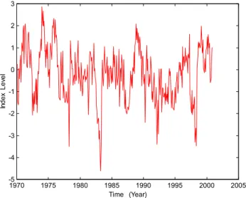
The data set used in this analysis is the monthly- average SOI time series extending from January 1866 through Decem-ber 2000, with a sampling interval of one month (Mitchell, 1999). This gives a data set of 1620 samples. Figure 1 shows the SOI data from January 1970 to October 2000. If SOI’ is normalized sea-level pressure (SLP) at Tahiti minus
normal-342 J. I. Salisbury and M. Wimbush: Using modern time series analysis techniques to predict ENSO events 1 2 -2 0 2 c1 . -1 0 1 c2 -1 0 1 c3 1880 1900 1920 1940 1960 1980 2000 -1 0 1 2 c4 YEAR 1970 1975 1980 1985 1990 1995 2000 2005 -5 -4 -3 -2 -1 0 1 2 3 Time (Year) In dex Lev el
Fig. 1. Monthly SOI data series from January 1970 to October 2000.
Tick marks on the time axis indicate the beginning of the designated year.
ized SLP at Darwin, then SOI is SOI’ normalized by its stan-dard deviation during 1951–1980. Prior to 1933 there were a few gaps in either the Tahiti or Darwin data; these range in length from 3 to 40 months. Since none of these gaps occur simultaneously at both locations, each gap has been filled by using the normalized pressure at the operating site with the appropriate sign, + for Tahiti, – for Darwin (Ropelewski and Jones, 1987; Allan et al., 1991; Konnen et al., 1998). These filled-in gaps that occurred more than 65 years ago should contribute relatively little to the prediction error.
3 Hilbert-EMD analysis
In this paper, we use a new data analysis method known as Empirical Mode Decomposition (EMD), in which a time series is decomposed into a set of intrinsic mode functions (IMF) derived from the data itself (Huang et al., 1998, 1999). The decomposition is based on the direct extraction of en-ergy associated with various intrinsic time scales. The local energy and instantaneous frequency derived from the IMFs through the Hilbert transform can give us a full energy-frequency-time distribution of the data. Such a representa-tion is designated as the Hilbert spectrum; it is well-suited to the analysis of nonlinear and nonstationary data.
With this method, we can localize an event in both time and frequency. The decomposition can be viewed as an ex-pansion of the data in terms of the IMFs. These functions are almost orthogonal, and form a complete basis: the sum of the IMFs equals the original data. The IMFs can be lin-ear or nonlinlin-ear, as dictated by the data. Most important of all, the expansion is adaptive. Locality and adaptivity are the necessary features of a basis for expanding nonlinear and nonstationary time series.
To compute an intrinsic mode function from a data set
x(t ), one first identifies the successive extrema of x(t), then 1 2 -2 0 2 c1 . -1 0 1 c2 -1 0 1 c3 1880 1900 1920 1940 1960 1980 2000 -1 0 1 2 c4 YEAR 1970 1975 1980 1985 1990 1995 2000 2005 -5 -4 -3 -2 -1 0 1 2 3 Time (Year) In dex Lev el
Fig. 2. SOI Intrinsic Mode Functions C1, C2, C3, C4for the SOI
data set. 3 6 -1 0 1 c5 -0.4 -0.2 0 0.2 0.4 c6 -0.2 0 0.2 c7 1880 1900 1920 1940 1960 1980 2000 -0.05 0 0.05 c8 YEAR 1970 1975 1980 1985 1990 1995 2000 2005 -5 -4 -3 -2 -1 0 1 2 3 4 Time (Year) In dex Lev el
Fig. 3. Same as Fig. 2, but for Intrinsic Mode Functions
C5, C6, C7, C8.
the local maxima are connected by a cubic spline as the up-per envelope, and the local minima are similarly connected as the lower envelope. The mean of these two envelopes is a function of time and designated as m1(t ). The difference between the data x(t ) and the mean m1(t )is computed and designated h1(t ) = x(t ) − m1(t ). This h(t ) is approximately the first IMF. To determine it more accurately, we treat h1(t )
as a new set of data, determine its upper and lower envelopes and compute their new mean, m11(t ), as well as the
differ-ence h11(t ) = h1(t ) − m11(t ). This h11(t )is again treated
as a new data set, and the process, referred to as “sifting,” is repeated a number of times. The sifting process is stopped when the number of zero-crossings of h1kequals the number
of extrema. The convergent result is designated by C1(t ),
which is the first IMF of the data set x(t); it has a zero local mean.
J. I. Salisbury and M. Wimbush: Using modern time series analysis techniques to predict ENSO events 343 difference, “the first residue”:
R1(t ) = x(t ) − C1(t ). (1)
The residue is analyzed by the same method as if it were new data. A new mean is found and the difference, R1(t )
minus its mean, converges to a function of time, C2(t ), which
is the second intrinsic mode function of x(t). It also has a zero local mean. The second residue,
R2(t ) = R1(t ) − C2(t ), (2)
is formed, and the process is continued until either Cnor Rn
becomes so small that it is less than a predetermined value of substantial consequence, or the residue Rnbecomes a
mono-tonic function from which no more IMFs can be extracted. In the real world, the data set to be analyzed is generally noisy, nonstationary and of limited duration. These three fac-tors greatly limit our ability to distinguish whether, for exam-ple, the dynamical system is a random process, a low-order noisy chaotic system or a high-order chaotic system. If the signal of interest is captured in a single IMF, we can examine the predictability of this IMF.
The IMFs for the SOI data, computed using the sifting pro-cess described above, are presented in Figs. 2 and 3. C9is
the final residue; it shows a monotone trend. As can be seen,
C1 is composed of the smallest time scales, or highest
fre-quencies, and the time scale increases as the index i of Ci
increases. IMFs 1 through 5 contain the major portion of the energy in the SOI signal.
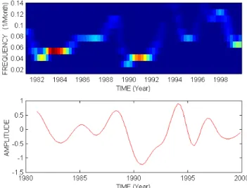
A few cycles of the Hilbert transforms of IMFs 3 and 4 are presented in Figs. 4 and 5. Intrawave modulation can be ob-served in both these figures. This behaviour is characteristic of nonlinear dynamics. Also, note that IMF 4 has a char-acteristic frequency of 0.03 cpm, which roughly corresponds to the 3.6-year mean interval between ENSO warm events. Figure 6 presents a comparison of the SOI and IMF 4 data for the years January 1970 to October 2000. IMF 4 resem-bles a smoothed version of the SOI data. We will attempt to use both the SOI time series and the IMF 4 series to predict ENSO events.
4 Prediction
We must now select an effective dynamical model, which will allow us to predict the evolution of any new point in the phase space within the limits of the intrinsic instabilities em-bodied in the data. The basic idea is that since we know ap-proximately how points in a neighborhood evolve into points in the next neighborhood, we can make a predictive estimate using an appropriate function, G, such that
ˆ
ζ (n +1) = G(ζ (n)) . (3)
Using the techniques described by Kantz and Schreiber (1997), various functions for predicting future events of non-linear dynamical systems were employed on the SOI and IMF 4 data. Various options, input parameter values and prediction models were tried. Evaluation was performed by
Fig. 4. The Hilbert spectrum (upper panel) from IMF 3 (lower
panel) of the SOI for the period 1982–2000. Note the intrawave modulation in which the local frequency varies within the domi-nant cycle of the oscillation.
Fig5
Fig. 5. Same as Fig. 4, but for IMF 4. 3 6 -1 0 1 c5 -0.4 -0.20 0.2 0.4 c6 -0.2 0 0.2 c7 1880 1900 1920 1940 1960 1980 2000 -0.05 0 0.05 c8 YEAR 1970 1975 1980 1985 1990 1995 2000 2005 -5 -4 -3 -2 -1 0 1 2 3 4 Time (Year) In dex Lev el
Fig. 6. Monthly SOI data series (red) from January 1970 to
Oc-tober 2000. Also, the IMF 4 data series for the same time period. Tick marks on the time axis indicate the beginning of the desig-nated year.
344 J. I. Salisbury and M. Wimbush: Using modern time series analysis techniques to predict ENSO events 7 8 1997 1997.5 1998 1998.5 1999 1999.5 2000 2000.5 2001 -4 -3 -2 -1 0 1 2 Time (Year) In dex Lev el 1992 1993 1994 1995 1996 1997 1998 1999 -1.5 -1 -0.5 0 0.5 1 1.5 Time (Year) In dex Lev e l
Fig. 7. 48-month prediction (blue) based on the measured SOI data
prior to 1997. Actual SOI time series for the 1997–2000 period of the prediction is also shown (red).
looking at both the in-sample and out-of-sample errors. We selected the prediction algorithm and the combination of em-bedding dimension and delay resulting in the smallest out-of-sample error. The functional form selected, which is flex-ible enough to model the true function on the whole attractor, is a multivariate polynomial (Giona et al., 1991), which for degree h and dimension d has k = (d + h)!/(d!h!) inde-pendent coefficients. The problem to be solved, given the
N d-dimensional vectors
(x(1), x(2), . . . , x(N )) , (4) is to reconstruct the mapping,
x(n + 1) = F (x(n)), (5)
where F is a d-dimensional vector of polynomial functions of the d components of x.
The combination of an embedding dimension of 4, a delay of 1 month, and a third-degree polynomial, gave the smallest out-of-sample error. All techniques and parameters resulted in predicted variations occurring at a slightly lower frequency than those observed.
We first used the SOI data without the last 48 data points, January 1997 to December 2000, to make a prediction for these four years. The period from January 1866 to Decem-ber 1996 was used as a training set to predict 48 months into the future. The results are depicted in Fig. 7, which shows a nearly useless prediction (blue), giving a proper value only for the mean, as expected for a random process.
Next, the Hilbert-EMD procedure was carried out on the SOI data to obtain IMF 4 for the period January 1866 – cember 1994, and again for the period January 1866 – De-cember 1995. The same scheme was used to predict the suc-ceeding 48 month period in each case, January 1995 – De-cemeber 1998 (Fig. 8) and January 1996 – December 1999 (Fig. 9). Both of these predictions show a strong “cold event”
7 8 1997 1997.5 1998 1998.5 1999 1999.5 2000 2000.5 2001 -4 -3 -2 -1 0 1 2 Time (Year) In dex Lev el 1992 1993 1994 1995 1996 1997 1998 1999 -1.5 -1 -0.5 0 0.5 1 1.5 Time (Year) In dex Lev e l
Fig. 8. 48-month prediction (blue) of IMF 4 computed from SOI
data prior to 1995 (red).
9 10 1992 1993 1994 1995 1996 1997 1998 1999 2000 -1.5 -1 -0.5 0 0.5 1 1.5 Time (Year) In dex Lev e l 1997 1998 1999 2000 2001 2002 2003 2004 2005 -1.5 -1 -0.5 0 0.5 1 1.5 Time (Year) In dex Lev el
Fig. 9. 48-month prediction (blue) of IMF 4 computed from SOI
data prior to 1996 (red).
9 10 1992 1993 1994 1995 1996 1997 1998 1999 2000 -1.5 -1 -0.5 0 0.5 1 1.5 Time (Year) In dex Lev e l 1997 1998 1999 2000 2001 2002 2003 2004 2005 -1.5 -1 -0.5 0 0.5 1 1.5 Time (Year) In dex Lev el
Fig. 10. 48-month (2001–2004) prediction (blue) of IMF 4
with the observed SOI index (Fig. 7, red curve), except that the predicted times for these events are somewhat later than the observed times, as a result of the frequency shift men-tioned above. Now using the IMF 4 data derived from all available SOI data up to December 2000, a 48-month, Jan-uary 2001 – December 2004 prediction was made; it is pre-sented in Fig. 10. The actual measured data, including the past warm and cold events, are plotted (red) along with the predicted (blue) results, which begin after the last known data point (December 2000). The predicted SOI magnitudes from January 2001 to December 2004 are all less than one, indi-cating that no strong warm or cold events are predicted by this procedure before December 2004.
5 Conclusion
It has been shown that the Empirical Mode Decomposition separates the total dynamics in the SOI into a finite number of simpler components. Attempting to predict future events using the undecomposed data proved fruitless. By analyzing just one of the EMD components, IMF 4, which has the same mean frequency as ENSO, we have been able to study a much simpler dynamical system and predict future events.
Out-of-sample predictions based on the 4th Intrinsic Mode Function of the SOI data show a strong warm event in 1997– 1998 and a strong cold event in 1999, as observed. They also forecast no strong ENSO events during the period 2001– 2004.
further extension of the Tahiti-Darwin SOI, early ENSO events and Darwin pressure, J. Climate, 4, 743–749, 1991.
CPC (Climate Prediction Center, NOAA): Experimental Long-Lead Forecast Bulletin, 6, No. 1, March, 1992.
Giona, M., Lentini, F., and Cimagalli, V.: Functional reconstruc-tion and local predicreconstruc-tion of chaotic time series, Phys. Rev. A, 44, 3496–3502, 1991.
Huang, N. E., Shen, Z., Long, S. R., Wu, M. C., Shih, H.-H., Zheng, Q., Yen, N.-C., Tung, C.-C., and Liu, H.-H.: The empirical mode decomposition and the Hilbert spectrum for nonlinear and non-stationary time series ananlysis, Proc. Roy. Soc. London Ser. A, 454, 903–995, 1998.
Huang, N. E., Shen, Z., and Long, S. R.: A new view of nonlin-ear water waves: the Hilbert spectrum, Annual Review of Fluid Mechanics, 31, 417–457, 1999.
Kantz, H. and Schreiber, T.: Nonlinear Time Series Analysis, Cam-bridge University Press, 1997.
Konnen, G. P., Jones, P. D., Kaltofen, M. H., and Allan, R. J.: Pre-1866 extensions of the Southern Oscillation Index using early Indonesian and Tahitian meteorological readings, Journal of Cli-mate, 11, 2325–2339, 1998.
Mitchell, T.: Southern Oscillation Index,http://tao.atmos. washington.edu/pacs/additional_analyses/ soi.html, 1999.
Philander, S. G.: El Ni˜no, La Ni˜na, and the Southern Oscillation, Academic Press, San Diego, 1990.
Ropelewski, C. F. and Jones, P. D.: An extension of the Tahiti-Darwin Southern Oscillation Index, Monthly Weather Review, 115, 2161–2165, 1997.