HAL Id: hal-03201039
https://hal.archives-ouvertes.fr/hal-03201039
Submitted on 18 Apr 2021
HAL is a multi-disciplinary open access
archive for the deposit and dissemination of
sci-entific research documents, whether they are
pub-lished or not. The documents may come from
teaching and research institutions in France or
abroad, or from public or private research centers.
L’archive ouverte pluridisciplinaire HAL, est
destinée au dépôt et à la diffusion de documents
scientifiques de niveau recherche, publiés ou non,
émanant des établissements d’enseignement et de
recherche français ou étrangers, des laboratoires
publics ou privés.
from the deep ocean and their dependence on the
Meridional Overturning Circulation
J. Palter, J. Sarmiento, A. Gnanadesikan, J. Simeon, R. Slater
To cite this version:
J. Palter, J. Sarmiento, A. Gnanadesikan, J. Simeon, R. Slater. Fueling export production: nutrient
return pathways from the deep ocean and their dependence on the Meridional Overturning Circulation.
Biogeosciences, European Geosciences Union, 2010, 7 (11), pp.3549-3568. �10.5194/bg-7-3549-2010�.
�hal-03201039�
www.biogeosciences.net/7/3549/2010/ doi:10.5194/bg-7-3549-2010
© Author(s) 2010. CC Attribution 3.0 License.
Biogeosciences
Fueling export production: nutrient return pathways from
the deep ocean and their dependence on the Meridional
Overturning Circulation
J. B. Palter1, J. L. Sarmiento1, A. Gnanadesikan2, J. Simeon3, and R. D. Slater1
1Atmospheric and Oceanic Sciences Program, Princeton University, Princeton, New Jersey, USA 2Geophysical Fluid Dynamics Laboratory, Princeton, New Jersey, USA
3Laboratoire des Sciences du Climat et de l’Environnement, CEN Saclay, 91191 Gif-sur-Yvette, France Received: 9 May 2010 – Published in Biogeosciences Discuss.: 1 June 2010
Revised: 30 September 2010 – Accepted: 8 October 2010 – Published: 10 November 2010
Abstract. In the Southern Ocean, mixing and upwelling
in the presence of heat and freshwater surface fluxes trans-form subpycnocline water to lighter densities as part of the upward branch of the Meridional Overturning Circulation (MOC). One hypothesized impact of this transformation is the restoration of nutrients to the global pycnocline, with-out which biological productivity at low latitudes would be significantly reduced. Here we use a novel set of modeling experiments to explore the causes and consequences of the Southern Ocean nutrient return pathway. Specifically, we quantify the contribution to global productivity of nutrients that rise from the ocean interior in the Southern Ocean, the northern high latitudes, and by mixing across the low lati-tude pycnocline. In addition, we evaluate how the strength of the Southern Ocean winds and the parameterizations of subgridscale processes change the dominant nutrient return pathways in the ocean. Our results suggest that nutrients upwelled from the deep ocean in the Antarctic Circumpolar Current and subducted in Subantartic Mode Water support between 33 and 75% of global export production between 30◦S and 30◦N. The high end of this range results from an ocean model in which the MOC is driven primarily by wind-induced Southern Ocean upwelling, a configuration favored due to its fidelity to tracer data, while the low end results from an MOC driven by high diapycnal diffusivity in the py-cnocline. In all models, nutrients exported in the SAMW layer are utilized and converted rapidly (in less than 40 years)
Correspondence to: J. B. Palter ([email protected])
to remineralized nutrients, explaining previous modeling re-sults that showed little influence of the drawdown of SAMW surface nutrients on atmospheric carbon concentrations.
1 Introduction
Primary productivity in the ocean’s sunlit surface incorpo-rates dissolved nutrients into organic matter, a fraction of which sinks to the ocean interior. Once in the ocean’s dark interior, the organic matter is respired back to dissolved in-organic carbon and nutrients, thereby creating the pervasive vertical nutrient and carbon gradients that characterize the global ocean. In and above the pycnocline (nominally above the 1026.8 kg m−3potential density surface), the total inven-tory of phosphate, an essential nutrient for photosynthesis, is approximately 150 Tmol (Conkright et al., 2001). Recent es-timates of the sinking flux of organic phosphorus (Dunne et al., 2007), propagated to the depth of this density surface, are of order 3 Tmol yr−1. Thus, to prevent the upper ocean from becoming entirely depleted of phosphate, the nutrient must be returned to the upper ocean on time scales of approxi-mately 50 years. We hypothesize that the upward branch of the Meridional Overturning Circulation (MOC), which con-verts dense deep waters to lighter pycnocline waters, plays a central role in maintaining the primary productivity of the upper ocean by returning exported nutrients to depths where they can again become accessible to the ocean’s sunlit upper reaches. On long time scales, the MOC’s upward branch bal-ances the sinking of deep waters and is driven by a combina-tion of vertical mixing across the low latitude pycnocline and
wind-driven upwelling and mixing in the Southern Ocean (Kuhlbrodt et al., 2007). However, the relative magnitude of the low latitude pathway versus the Southern Ocean path-way remains an open question, as does the implication for the cycling of nutrients. Here, we explore the MOC nutrient re-turn pathways in a suite of ocean general circulation models with different physical parameterizations, seeking an under-standing of the balance between the Southern Ocean nutrient pathway versus the low latitude pathway and the sensitivity of this balance to model physics.
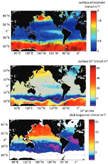
A dominant role for the Southern Ocean in the MOC’s up-ward branch has formerly been hypothesized based on tracer data (Toggweiler et al., 1991; Sarmiento et al., 2004, 2007) in the context of theoretical considerations of ocean overturn-ing (Toggweiler and Samuels, 1995, 1998; Gnanadesikan, 1999). In terms of nutrient cycling, this hypothesis implies a loop in which the global loss of organic matter to depths be-neath the pycnocline is largely balanced by the upwelling of remineralized nutrients in the Antarctic Circumpolar Current (ACC). These nutrients are then advected and mixed across the ACC into the Subantarctic Mode Water (SAMW), a wa-ter mass formed on the ACC’s equatorward fringes that in-fluences tracer properties throughout much of the global py-cnocline (McCartney, 1982; Sarmiento et al., 2004; Hanawa and Talley, 2001). This conceptual model hinges on the up-welled nutrients being subducted with the SAMW at the time it forms, rather than being utilized and exported from it, as can be the case for other mode waters (Palter et al., 2005). Indeed, the SAMW is formed in a region with highly ele-vated surface nutrients (Fig. 1a), and it tends to retain its nu-trients during formation and subduction. Evidence support-ing the dominance of the Southern Ocean nutrient upwellsupport-ing pathway has been obtained by model sensitivity studies, in which the strength of global primary production was criti-cally reduced by completely stripping nutrients from the sur-face ocean in the SAMW formation region (Sarmiento et al., 2004; Marinov et al., 2006).
Additional support for the importance of a Southern Ocean upward MOC branch in influencing pycnocline nutrient con-centrations comes from looking at quasi-conservative com-binations of nutrient tracers. For example, in the Subantarc-tic Zone where SAMW is formed, phosphate (PO3−4 ) and nitrate (NO−3) are abundant, while silicic acid (Si(OH)4) is nearly depleted. Thus, a useful tracer of the SAMW is Si∗=Si(OH)4-NO−3 (Sarmiento et al., 2004). The lowest Si∗ concentrations in the global surface ocean are found in the SAMW formation region (Fig. 1b). Sarmiento et al. (2004) argue that because Si∗ is approximately conserved in the ocean interior, the subsurface pool of negative Si* indicates the spreading of SAMW via advective and diffusive transport processes throughout much of the South Pacific, Indian and low latitude Atlantic Oceans (Fig. 1c).
Fig. 1. Global nutrients at the ocean’s surface and in the SAMW
layer. (a) Surface phosphate from WOA01 (Conkright et al., 2001). (b) Surface Surface Si∗=Si(OH)4-NO−3 from WOA01. (c) Si∗on the 26.8 isopycnal, at the center of the SAMW layer. In panels (a) and (b), black hatches indicate regions between 65◦S and 65◦N where annual maximum mixed layer depths exceed 400 m, where mixed layer depths are taken from de Boyer Mont´egut et al. (2004). Panel (c) is recreated after Sarmiento et al. (2004). The white area represents the region where the annual mean surface density ex-ceeds 1026.8 kg m−3
Despite the apparent convergence of evidence from mod-els and the Si∗ tracer towards a central role for a Southern Ocean nutrient return pathway from the deep ocean to the pycnocline, several important questions still require evalu-ation and quantificevalu-ation. What is the fraction of low lat-itude productivity sustained by the Southern Ocean nutri-ent return pathway and which water masses are involved? In which regions are the SAMW nutrients most impor-tant, and what are the pathways by which the SAMW ar-rives at these downstream locales? Here we examine these questions using a suite of ocean general circulation models (OGCMs). A second class of questions concerns the sen-sitivity of the predominant nutrient return pathway to the
models’ parameterizations of subgridscale processes and the prescribed atmospheric forcing that drives the ocean circula-tion, particularly the Southern Ocean winds. The fraction of deep upwelling that occurs in the Southern Ocean is sensitive to the strength of the winds, as well as the turbulent mixing and transport due to mesoscale eddies, which are parameter-ized in the coarse GCMs typically used to simulate climate and biogeochemistry. The sensitivity of the modeled MOC to winds and subgridscale processes has been demonstrated in more than one idealized analytical model (Gnanadesikan, 1999; Samelson, 2004, 2009), and tested in a suite of GCMs (Gnanadesikan et al., 2007). Here we quantify the sensitivity of the magnitude and distribution of nutrient supply to wind forcing and the parameterizations of subgridscale processes. We also consider the implication of these results for non-steady behavior by investigating the lateral and temporal scales over which the preformed nutrients subducted in the SAMW layer persist in the ocean interior before fueling downstream primary productivity. Preformed nutrients are those inorganic nutrients that enter the ocean interior with-out having fueled primary productivity while in the mixed layer. Therefore, preformed nutrients are a signature of inef-ficiency in the biological pump. A more efficient biological pump utilizes a greater portion of surface nutrients, converts them to organic material and increases the remineralized nu-trient and carbon concentration deeper in the water column. Higher remineralized nutrient concentrations signify greater ocean carbon storage and lower atmospheric carbon diox-ide, while a higher preformed nutrient inventory signals a smaller ocean carbon reservoir (Archer et al., 2000; Ito and Follows, 2005; Gnanadesikan and Marinov, 2008; Marinov et al., 2008a, b). Much of the SAMW nutrients enter the ocean in their preformed state, but when they fuel produc-tivity downstream of their formation region, these inorganic nutrients are incorporated to organic matter and eventually converted to their remineralized state. Any increase in the subduction of the SAMW preformed nutrient pool would di-minish the deep ocean carbon reservoir until these preformed nutrients are converted to their remineralized form. Evalua-tion of this potential for change in the ocean preformed nu-trient reservoir is especially timely given recent observations showing the intensification of Southern Hemisphere westerly wind strength (Thompson and Solomon, 2002) with implica-tions for the stability of the ocean carbon sink (Le Qu´er´e et al., 2007). Such an intensification is expected to increase the cross-ACC Ekman transport of preformed nutrients, the pre-formed nutrient load of the SAMW, and the local inefficiency of the biological pump due to the subducted preformed nu-trients in the mode and intermediate waters. Our model ex-periments shed light on the time scale that this perturbation might be expected to persist.
2 The theory, the models, and the experimental design 2.1 The theory
A simple conceptual model of the MOC consists of four branches: (1) deep water formation regions in the North At-lantic where surface waters become denser and sink; (2) flow away from these regions at depth; (3) upwelling and mix-ing that transports the dense waters from the ocean interior to the surface ocean; and (4) near-surface currents that close the circulation. Where and by what forcing mechanism the deep water returns to the surface (branch 3) is a central ques-tion in physical oceanography (for an extensive review see Kuhlbrodt et al., 2007), and, increasingly, motivates ocean biogeochemical and climate studies (Gnanadesikan et al., 2002; Sarmiento et al., 2007; Anderson et al., 2009). The two forcing mechanisms that have received the most attention are the downward mixing of heat and associated upwelling across the pycnocline (see Munk and Wunsch, 1998 for a detailed discussion) and the wind-driven upwelling of deep waters in the Southern Ocean and their subsequent buoyancy gain at the surface of the ocean (Toggweiler and Samuels, 1993, 1995). Gnanadesikan (1999) proposed a simple model that nicely synthesizes these two mechanisms into a single framework by relating the large-scale MOC to winds, ed-dies, and diapycnal mixing, as schematized in Fig. 2. The un-derpinning of the theory is that along-isopycnal eddy trans-port, diapycnal mixing, and wind forcing all determine where dense water returns to the ocean’s surface, while the interplay of all three factors determines the depth and thickness of the pycnocline and the strength of the overturning cell.
For the modern ocean, the Gnanadesikan (1999) theory can be summarized as follows. Dense water forms and sinks in the high latitude North Atlantic and is exported south-ward in the deep limb of the MOC, a flux represented in the schematic as Mn. All along its export pathways, the down-ward mixing of heat transforms the dense water to lighter densities and forces an upward volume flux represented as Mu that reduces the deep southward flow as it approaches the Southern Ocean. This upward flux scales as:
Mu =
KvA
D , (1)
where Kvis the coefficient of diapycnal diffusion, D is the pycnocline depth that separates dense water from light, and Ais the area of the low latitude pycnocline.
In the Southern Ocean, laterally divergent Ekman trans-port forces the upwelling of abyssal waters, a flux repre-sented as Ms. The upwelled waters that cross the ACC into the SAMW formation region gain buoyancy along their journey, thus completing the dense-to-light transformation of the water masses formed in the North Atlantic. However, adding another layer of complexity, a volume transport due to mesoscale eddies is directed southward across the ACC, balancing some fraction of the northward Ekman transport.
Depth S Latitude Northern sinking Low latitude upwelling & mixing, Mu Shallow northward transport, Mn Wind-driven flow Eddy return flow
N Kv Ai b) σθ < 27.4 Low Kv, Low Ai (LL) High Kv, High Ai (HH) LL-ECMWF winds LL-ECMWF + tuning ∫∫v dx dz (S v) ∫∫v dx dz (S v) Latitude Southern Ocean upwelling and mixing, Ms τx a) c) σθ > 27.4 Depth S Latitude Northern sinking Low latitude upwelling & mixing, Mu Shallow northward transport, Mn Wind-driven flow Eddy return flow
N Kv Ai b) σθ < 27.4 Low Kv, Low Ai (LL) High Kv, High Ai (HH) LL-ECMWF winds LL-ECMWF + tuning ∫∫v dx dz (S v) ∫∫v dx dz (S v) Latitude Southern Ocean upwelling and mixing, Ms τx a) c) σθ > 27.4
Fig. 2. Schematic of the simple analytical model of the Meridional Overturning Circulation (MOC) and the model results of the MOC. (a) Adapted from Gnanadesikan (1999), the schematic of the flows (gray arrows) which comprise the MOC and their driving mechanisms
(boxed text). The black line schematizes the global pycnocline, below which nutrient-rich water is found, represented by green shading. The sinking of water masses in the Northern Hemisphere is balanced by the sum of the Southern Ocean upwelling (Ms) and low latitude upwelling (Mu). The rate of Southern Ocean upwelling is set by the wind stress over the Southern Ocean (τx) and the eddy return flow, which is determined largely by the GM coefficient (Ai). The low latitude upwelling is driven by the downward mixing of heat, which is set by the vertical mixing coefficient (κv). (b) The zonally integrated meridional transport above the 27.4 isopycnal (northward is positive) for each of the four models described in Table 1. (c) The same as panel (b), but below the 27.4 isopycnal. By design, panels (b) and (c) are mirror images of one another because the total transport sums to zero for the volume-conserving ocean of the GCMs. A meridional increase in the meridional transport above (below) the 27.4 isopycnal signals the upwelling (downwelling) of water across the 27.4 isopycnal. The four models are described in Sect. 2.2 of the text and in Table 1.
The eddy transport is thought to be proportional to the local slope of isopycnals, which is the source of potential energy from which the eddies grow (Gent and McWilliams, 1990). Thus, the flux of abyssal water to the light water realm in the Southern Ocean, Ms, is equal to the difference between the Ekman transport Mekand the residual mass flux due to the eddies: Ms = Mek − AiDLx LS y (2) where Ai is a coefficient that determines the strength of the eddy mass transport, LSyis the north-south scale over which the pycnocline shallows in the Southern Ocean, and Lxis the Earth’s circumference at the Drake Passage latitude (see also Karsten and Marshall, 2002).
For the limiting case in which the eddy transport across the ACC is as large as the Ekman transport, the net South-ern Ocean deep water return pathway becomes negligi-ble and the upward branch of the MOC must be accom-plished exclusively through low latitude diapycnal mixing; this is the picture of the MOC hypothesized by Stommel and Arons (1961). For the alternate limiting case in which
global diapycnal mixing is, on average, as small as the di-apycnal mixing measured in the ocean away from topogra-phy (Gregg and Sanford, 1980; Ledwell et al., 1993, 1998), the Ekman upwelling of dense waters in the Southern Ocean and their buoyancy gain provide the primary driver of merid-ional overturning (Toggweiler and Samuels, 1998). We note that this conceptual model does not explicitly consider spa-tial variability in the strength of diapycnal mixing observed in the ocean (Heywood et al., 2002; Naveira Garabato et al., 2004), although the model framework outlined below allows for some exploration of this variability.
2.2 The models
The underlying architecture used to probe our questions is a suite of simulations using the Geophysical Fluid Dynam-ics Laboratory Modular Ocean Model version 3 (MOM3) (Pacanowski and Griffies, 1999). The MOM3 suite explores a range of mixing parameters and wind forcing, as described in several previous studies (Gnanadesikan, 1999; Gnanade-sikan et al., 2004, 2007; Mignone et al., 2006), and sum-marized in Table 1. The models create variants of the MOC
Table 1. Description of the four ocean GCMs. Model acronyms are described in the text. Differences from LL are highlighted in italic. Configuration: LL (Low diapycnal diffusivity; Low GM coefficient) HH (High diapycnal diffusivity; High GM coefficient) LL-ECMWF (Low diapycnal diffusivity; Low GM coefficient; ECMWF winds, stronger in S. Ocean) P2A
(Low diapycnal diffusivity outside the top 50 m; Low GM coefficient; ECMWF winds, stronger in S. Ocean; several additional modifications) Diapycnal diffusivity (tropics) (m2s−1) 1.5 × 10⁻⁵ 6 × 10⁻⁵ 1.5 × 10⁻⁵ 1.5 × 10⁻⁵ Diapycnal diffusivity (Southern Ocean) (m2s−1) 1.5 × 10⁻⁵ 6 × 10⁻⁵ 1.5 × 10⁻⁵ 13 × 10−5 Enhanced diffusivity in top 50 m No No No Yes Along isopycnal diffusivity AND coefficient for GM thickness diffusion (m2s−1) 1000 2000 1000 1000 Applied surface moisture fluxes
Da Silva et al. (1994) Da Silva et al. (1994) Da Silva et al. (1994) Da Silva et al. (1994) plus correction globally Temperature and
salinity toward which restoring occurs
Levitus et al. (1994) Levitus et al. (1994) Levitus et al. (1994) Levitus et al. (1994) plus correction factor near Antarctica in winter
Wind stress Hellerman Hellerman ECMWF ECMWF
Topography Wide Drake Passage Wide Drake Passage Wide Drake Passage Narrow Drake Passage
strength and structure by changing: (a) the Southern Ocean Ekman transport, Mek, via the use of two different wind re-analysis products to force the model; (b) the counterbalanc-ing eddy transport via the manipulation of Ai, the coefficient associated with the Gent and McWilliams (1990) (GM) pa-rameterization of eddy transport; and (c) the diapycnal mix-ing across the low latitude pycnocline via variations in Kv, the coefficient of diapycnal diffusion. Here we present the results from a subset of four models from a larger MOM3 suite explored in Gnanadesikan et al. (2007), chosen because they capture much of the inter-model differences of the full parameter range without being excessively cumbersome for comparison.
Two of the models are forced with wind stresses from Hellerman and Rosenstein (1983), which are approximately half as intense in the Southern Ocean as the European Cen-tre for Medium-Range Weather Forecasts (ECMWF) clima-tological winds (Trenberth et al., 1989) used to force the other two models. Of these Hellerman and Rosenstein-forced models, one is run with a Low Kvand Low Ai, and is there-fore referred to as LL; the other has a High Kvand High Ai,
and is referred to as HH. LL-ECMWF is identical to the LL model in the ocean, but is forced with ECMWF winds. A special case we call P2A resembles the LL-ECMWF model but has been modified in several ways intended to increase the realism of the simulation: the Drake Passage was nar-rowed from three grid points (1165 km) to two (777 km) to be closer to the real Drake Passage, which is 800 km wide; strong vertical mixing (5 × 10⁻³m2s−1) is imposed on the uppermost two grid cells (50 m) as a very crude approxi-mation to what actually occurs in an oceanic mixed layer; and surface salinity is strongly restored to subsurface obser-vations in four key locations at the onset of Austral winter in Southern Ocean deep water formation regions to simu-late brine rejection during sea-ice formation. Without this salinity adjustment, restoring the model to observations sup-presses Antarctic Bottom Water (AABW) formation, as the observations do not capture the outcropping of such wa-ters. Finally, in P2A the coefficient of diapycnal mixing is increased in the Southern Ocean, first motivated by ob-servations of intense ACC internal wave activity (Polzin, 1999) and later validated by observations of rapid diapycnal
tracer spreading in the region (Naveira Garabato et al., 2004). Clearly the MOC strength and upward branch is controlled by the interplay of these parameter choices (Fig. 2b–c), with the MOC in the HH model confined entirely to the region north of 20◦N, while the LL-ECMWF overturning is actu-ally intensified in the Southern Hemisphere. We will explore the MOC differences among the models at greater length in Sect. 3.
A model of the biological cycling of phosphorus and car-bon is coupled to the physical model, as specified by the Ocean Carbon Model Intercomparison Project-2 (OCMIP-2) protocol (Najjar et al., 2007). In this protocol, phospho-rus is the only simulated nutrient and is conserved globally in all experiments. The phosphorus source/sink terms are governed by an extremely simple set of equations meant to represent the incorporation of phosphate into organic mat-ter by photosynthesis in the euphotic zone and the sinking of this organic matter and its remineralization back to phos-phate throughout the water column (Fig. 3). The simulated phosphorus appears in 2 pools: dissolved organic phospho-rus (DOP) and phosphate (PO3−4 ). These pools are trans-ported as passive tracers by the physical model. At depths shallower than 75 m, the model PO3−4 in excess of a seasonal PO3−4 climatology (Louanchi and Najjar, 2000) fuels primary production, represented by restoring the surface model PO3−4 to climatological values over a time scale of τ = 30 days. The resulting production has two fates: two thirds becomes a source term for DOP and one third fuels a parameterized sinking flux of organic phosphorus that is shunted to 75 m. Below 75 m, the sinking flux decays as a function of depth and its vertical divergence is a source term of PO3−4 . DOP is remineralized to PO3−4 everywhere in the model, at a rate of κ =0.5 year−1.
2.3 The experimental design
To investigate the role of the upward branch of the MOC in the supply of nutrients to the low latitude pycnocline and ulti-mately the euphotic zone, we created two sets of tags that are schematized in Fig. 4. The first is a simple set of dye tracers. In each tagging region (represented in black in the schemat-ics), the dye value is set to one; in each destruction region (white in the schematics), the dye value is set to zero; in the rest of the domain (gray in the schematics), the dye tags are treated as conserved, passive tracers. The dyes are named according to their source locations and are fully described in Fig. 4 and its caption. The physical model is spun up to a steady circulation before the dyes are released. All presented results are averages between year 190 and 200 after the re-lease of the tags, except for LL-ECMWF, which are for years 390–400. The longer integration time for LL-ECMWF was chosen only because the appropriate terms were not archived until the later time period. At year 190, the drift in average low latitude dye concentrations is less than 0.1% year−1, very
Zc = 75 m Production
zone
Consumption zone
1) JProd=1τ [PO
(
4model]−[PO4Obs])
2) 0.67JProd=JDOP+κ[DOP] 3) F75=0.33 JProddz 0 75 m∫
7) JDOP= −κ[DOP] F(z) = F75 75z ⎛ ⎝ ⎜ ⎞ ⎠ ⎟ −0.9 JPO4= − dF (z)dz + κ[DOP]if[POmodel] [PO 4 Obs] > , 4 6) JPO= 4 κ[DOP] 4) 5) -JProd
Fig. 3. A schematic showing the governing equations of the OCMIP-2 biological model. Terms that begin with the letter J are source/sink terms (black text), while terms that begin with the letter F are flux terms (grey text). At depths shallower than 75 m, model PO3−4 (POmodel4 ) in excess of a seasonal climatology (POObs4 ) (Louanchi and Najjar, 2000) fuels new production (JProd), thus restoring the surface model to climatological values over a time scale of τ = 30 days (Eq. 1). The resulting productivity has two fates: two thirds becomes a source term for DOP (JDOP, Eq. 2), and one third fuels a parameterized sinking flux of organic phosphorus, that is shunted to 75 m (F75, Eq. 3). Below 75 m, the sinking flux decays as a function of depth (Eq. 4). The vertical divergence of this sinking flux is a source term of PO3−4 (Eq. 5). DOP is reminer-alized to PO3−4 everywhere in the model, at a rate of κ = 0.5 year-1 (Eqs. 5 and 6). This DOP to PO3−4 decay is a sink term for DOP (−κ[DOP], Eqs. 2 and 7).
close to equilibrium, and almost all regions are fully tagged. After 200 years, only the water masses of the Bay of Bengal are not fully tagged (thus, the global sum of all tags can be slightly less than 100%).
Outside the tagging and destruction regions (i.e. in and above the low latitude pycnocline), the dye tracers directly measure the fractions of water that derive from each tagging region. The abyssal ocean is tagged only in low latitudes and only at potential densities greater than 27.4 kg m−3, which is beneath the main thermocline in all models. The North-ern Hemisphere High latitudes are tagged everywhere north of 40◦N, and further designated as stemming from the North Atlantic and North Pacific basins. In the Southern Ocean, the tags are divided into density classes in order to approximate the contribution of SAMW and AAIW to the low latitude py-cnocline. By design, the southernmost tag is trapped in the Southern Ocean, and is used primarily to ensure that all water masses are tagged and a water mass budget can be balanced. In the Southern Ocean, AAIW is most commonly identi-fied as a salinity minimum along the 27.3 isopycnal. Because the SAMW is formed in large part by convective processes, it can be identified as a pycnostad, or region of low verti-cal density stratification. A comparison of our simulations
DEPTH DEPTH 200m DEPTH 200m DEPTH d) AAIW b) Deep a) Northern c) SAMW N DEPTH 40oN 40oN 40oN 40oN 40oN 200m 200m 200m S N 26.5 27.1 27.4 S N 26.5 27.1 27.4 S N S N LATITUDE 26.5 27.1 27.4 N DEPTH 26.5 27.1 27.4 e) Southern 26.5 27.427.1 S
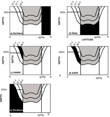
Fig. 4. A schematic of the experimental design used to examine
the nutrient return pathways to the low latitude surface ocean. Each panel represents the deployment of a regional tag in zonal cross-section. The curvy lines represent selected isopycnals, as labeled at the top of each panel. In the black area, the dye tag, phosphate, and DOP are tagged according to the following conventions: (a) The Northern tag (which was further subdivided into North Atlantic and North Pacific) set on all water north of 40◦N. (b) The Deep Low latitude tag, set for all water with potential densities greater than 27.4 between 40◦N and a southern boundary defined by the latitude where the 26.5 isopycnal intersects 200 m. (c) The SAMW tag, set between that same boundary and the 27.1 isopycnal. (d) AAIW tag, set between the 27.1 and 27.4 isopycnals southward of the same boundary. (e) Southern tag for all water denser than AAIW and southward of the boundary. In the white areas, the tag is destroyed and set to its new region. In the gray areas, all tags behave according to their conservation equation.
with a well-studied salinity and density section along 100◦E (Sloyan and Kamenkovich, 2007) (Fig. 5), reveals that the models do a good job simulating the salinity and stratifica-tion minima that characterize the AAIW and SAMW, respec-tively. The model density structure in the Southern Ocean re-sembles the observations, giving confidence that our South-ern Ocean water mass definitions are appropriate to address the question at hand. It is also reassuring that the SAMW dye tracer on the 26.8 isopycnal shows a similar spatial distribu-tion to the Si∗tracer from data (compare Fig. 6 with Fig. 1c). An exception to this similarity is in the degree of Atlantic-Pacific asymmetry. The Si∗tracer transitions to positive val-ues at the equator in the Pacific, possibly a consequence of mixing processes in the Sea of Okhotsk that are not resolved by the models (Talley, 1991; Sarmiento et al., 2004). We
note that the SAMW dye penetrates into the Northern Hemi-sphere in all of the models, regardless of whether there is net destruction or creation of light waters in the Southern Ocean. The differences among the models are largely seen in Indian Ocean, the equatorial Atlantic, and the western tropical Pa-cific where the HH model has 20–40% less SAMW than the others (Fig. 6).
The second set of tags is designed to trace nutrients from the same source regions as the dyes. In each source region, all model PO3−4 and DOP are tagged, or named according to their region, such that the total pools of PO3−4 and DOP ev-erywhere in the model domain are the sum of the regionally-tagged pools. As an illustrative example, PO3−4 and DOP are endowed with a SAMW tag between the 26.5 and 27.1 isopycnals in the Southern Hemisphere, southward of where the 26.5 isopycnal intersects 200 m (as for the SAMW dye tracer, shown in Fig. 4c).
As the SAMW-tagged DOP (hereafter SAMW DOP) is transported in the flow field from its tagging region, it is respired to a separate pool of remineralized SAMW phos-phate. The same is true for the SAMW phosphate that fu-els primary production downstream of its tagging domain: the remineralization of the resultant DOP and sinking flux provides a source of remineralized SAMW phosphate. Thus, although the phosphorus maintains its regional identity until it enters a destruction region, it is marked as either coming directly from the tagging region, which we will refer to as unmodified, or being created by remineralization away from the tagging region, which we refer to as remineralized. Un-modified nutrients in our experiments resemble preformed nutrients when they are tagged in the surface mixed layer and can shed light on the pathways and persistence of pre-formed nutrients in the ocean interior. Yet, we avoid the use of the word preformed to describe them, because the tags are not exclusively introduced in the mixed layer, and therefore our unmodified phosphate can differ from a traditional defi-nition of preformed nutrients. This distinction becomes par-ticularly apparent in our discussion of the unmodified deep low latitude phosphate, which is tagged only in the interior ocean, and therefore bears no resemblance to the traditional definition of preformed nutrients. Throughout this work, ref-erences to tagged nutrients and their unmodified and reminer-alized components will appear in italics for clarity.
In order to estimate the productivity sustained by the rem-ineralized tagged nutrients, Eqs. (2) and (6) from Fig. 3 are differenced to above 75 m to arrive at the expression:
JPRODtag = J tag DOP +J tag PO4 −0.33 (3)
This expression can be used to calculate the primary produc-tion fueled by each remineralized phosphate tag, JPRODtag . This result is divided by the total JPROD, which is archived by the model. According to this expression, a sink of PO3−4 (i.e. negative JPO4) is due to primary production, while a source
a) Observations b) LL c) HH
d) LL-ECMWF e) P2A
Salinity
Fig. 5. Salinity (colors) and density (contours) along 100◦E in (a) observations and (b–e) the 4 models, as labeled above each panel. The SAMW layer is visible as a pycnostad between the 26.5 and 27.1 isopycnals just north of the ACC, and the AAIW is characterized by a salinity minimum on the dense side of the SAMW. Observations taken from the CARS2006 database (Ridgway et al., 2002). Vertical lines show the time-mean boundary used to separate the SAMW tag region from the low-latitudes in the models.
of PO3−4 (due to the remineralization of DOP to PO3−4 ) is as-sociated with negative production. Thus, the total JPRODtag can be negative if the tagged DOP is remineralized to PO3−4 at a greater rate than the tagged remineralized PO3−4 fuels pro-ductivity.
3 Results and discussion 3.1 Model circulation
The simulated MOC in the different models behaves as pre-dicted by the simple analytical model presented in Sect. 2.1. In all models, the interplay of the chosen parameter values creates a pycnocline with a realistic depth and density and an MOC at 48◦N similar to the 16–19 Sv inferred from obser-vations (Table 2) (Lumpkin and Speer, 2007; Talley, 2008; Forget, 2010). However, the upward branch of the MOC
occurs at notably different locations among the models (Ta-ble 2). The LL model with its weak Southern Ocean winds and low mixing creates an MOC of 13.6 Sv, with more than half of the upward branch supplied in the Southern Ocean; the HH model creates 17.9 Sv of overturning, but its upward branch is realized entirely at low latitudes; and the P2A and LL-ECMWF models also yield over 18 Sv of overturning, but with upward branches primarily in the Southern Ocean. Some observationally-driven inverse models (Lumpkin and Speer, 2007) and, more recently, the results from the data-assimilating forward model used in Estimating the Circula-tion and Climate of the Ocean (ECCO) (Wunsch and Heim-bach, 2007; Forget, 2010) have suggested that the upward branch of the MOC is accomplished primarily in the South-ern Ocean (Table 2). Yet, another observationally-driven es-timate suggests a more important role for low latitude up-welling and implies values of low latitude diapycnal mixing
SAMW dye b) High-High
a) Low-Low
c) Low-Low-ECMWF d) P2A
Fig. 6. SAMW dye fraction on the 26.8 isopycnal for the 4 models described in Table 1 and labeled at the top of each panel.
as high as in our HH model (Talley, 2008). Thus, the rel-ative importance of these two possible upwelling branches lacks a definitive solution at present, providing a motivation for including in our analysis models that cover the range of possibilities. Furthermore, the modeled MOC has a direct influence on the large-range of air-sea CO2fluxes estimated from coupled models (Cao et al., 2009).
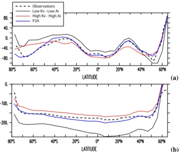
Radiocarbon, a useful tracer of ocean circulation, offers evidence consistent with the upwelling of deep waters in the Southern Ocean. We briefly compare the radiocarbon results from our four models with observations to offer a context with which to judge the various circulations. Radiocarbon enters the ocean only at the air-sea interface and then decays in the ocean interior with a half-life of 5730 years. Thus, the most-recently ventilated ocean waters are most enriched in radiocarbon, and the oldest waters most depleted. The HH model strongly mixes waters depleted in radiocarbon from the dense ocean interior to the surface in subtropical lati-tudes, causing a depleted radiocarbon bias in the near-surface layers (Fig. 7, red line). This bias is reversed in the South-ern Ocean, where the HH model overestimates the radiocar-bon in the surface due an excessive supply of low latitude, high radiocarbon surface waters. Not surprisingly, the LL model, which is also forced with sluggish Southern Hemi-sphere westerly winds but has weaker diapycnal diffusivity
and GM coefficients, has precisely the opposite bias: an un-derventilated deep ocean with a low radiocarbon bias, and corresponding radiocarbon trapping in the upper ocean. The P2A model with weak vertical mixing at low latitudes and high Southern Ocean winds and mixing is the most success-ful at accurately simulating the observed radiocarbon con-centrations in the surface and deep ocean (Fig. 7, blue line). The P2A model is also the only one with an ACC transport at Drake Passage (126 Sv) in the range of observational esti-mates of 135 ± 14 Sv (Cunningham et al., 2003); the other three models have a Drake Passage transport of approxi-mately 80 Sv. More extensive model-data comparison with the MOM3 suite can be found in a number of previous papers (Gnanadesikan et al., 2002, 2004; Matsumoto et al., 2004); all suggest a critical role for upwelling and/or mixing in the Southern Ocean in driving the MOC.
3.2 Spreading of dye and nutrient tags
Despite the differences among models, the SAMW com-prises a sizeable fraction (45–68%) of the low latitude wa-ters above the 26.8 isopycnal in all models (Table 3). As predicted in the analytical framework, the HH model has the smallest SAMW fraction, as water from depths beneath the pycnocline (with the Deep Low latitude tag) upwells directly
Table 2. Comparison of the pycnocline and MOC characteristics of the four models from the MOM3 suite and with estimates from
observa-tions.
Metric: LL HH LL-ECMWF P2A Estimates from observations (including inverse models and a data-assimilating forward model) Pycnocline depth (m)1 D = 2 2.5 km R 0 (σ1max−σ1)zdz 2.5 km R 0 (σ1max−σ1)dz 862 881 980 915 834
estimated from Conkright et al. (2001)
σθat pycnocline depth1 27.31 27.25 27.32 27.28 27.24
(Conkright et al., 2001) Mn(Sv): max northward
transport summed vertically from the surface at 48◦N
13.6 17.9 18.4 18.8 19 (Talley, 2008)2
18 (Lumpkin and Speer, 2007)2 16 (ECCO)3
Ms(Sv): transport at 32◦S above the 27.4 isopycnal
6.7 −3.7 15.9 12.2 −1.1 (Talley, 2008)
7.9 (Lumpkin and Speer, 2007) 15.8 (ECCO)3
Mu=Mn−Ms(Sv) 6.9 21.6 2.5 6.6 20.1 (Talley, 2008)2
10.1 (Lumpkin and Speer, 2007)2 0.2 (ECCO)3
1Averaged from 30◦S–40◦N;
2Estimated from inverse models at approximately 48◦N (M
n) and 32◦S (MS)using hydrographic data; details in Lumpkin and Speer (2007) and Talley (2008).
3Maximum global overturning at 48◦N and 32◦S calculated from the Ocean Comprehensive Atlas (OCCA), produced at the Massachusetts Institute of Technology (MIT) by the
Estimating the Circulation and Climate of the Ocean (ECCO) group. The OCCA Atlas is publicly available (http://www.ecco-group.org/) for the data-rich Argo period from 2004 to 2006 (Forget, 2010). OCCA is an ocean climatology produced by calculating the least squares fit of a global full-depth-ocean and sea-ice configuration of the MIT general circulation model (MITgcm) to satellite and in situ data.
Observations Low Kv - Low Ai P2A High Kv - High Ai (a) Observations Low Kv - Low Ai P2A High Kv - High Ai (b) Fig. 7. Zonal and depth-average δ14C above (a) and below (b) the 27.4 isopycnal for the observations from the GLODAP database (Key et al., 2004) and 3 of the 4 ocean models described in Ta-ble 1. The LL-ECMWF model is excluded, because it was not run with δ14C as a tracer.
Table 3. Percentage contribution of each tagged water mass to the
upper ocean volume (above the 26.8 isopycnal) between 30◦S and 30◦N in italic lettering. Listed in parentheses are the percentage contributions of unmodified tagged phosphate (first number) and the remineralized tagged phosphate (second number) to the total phos-phate inventory above the 26.8 isopycnal. The columnwise sum of the unmodified and remineralized contributions (both numbers in parentheses) should be close to 100% of the total phosphate reser-voir. However, some columns may sum to less than 100% due to roundoff error and because part of the Bay of Bengal is only par-tially tagged.
LL HH LL-ECMWF P2A
North Atlantic 5 (2, 3) 4 (1, 4) 5 (2, 2) 6 (3, 5)
North Pacific 24 (10, 22) 14 (5, 11) 16 (8, 16) 15 (6, 15)
Deep Low latitude 8 (9, 9) 33 (22, 21) 6 (6, 7) 5 (6, 5)
SAMW 60 (18, 21) 45 (12, 13) 68 (26, 28) 67 (24, 24)
AAIW 3 (2, 3) 4 (2, 4) 3 (2, 3) 2.5 (3, 4)
a) MOM3 HH - Total PO4 (mmol m3) b) World Ocean Atlas 2005 - PO4 (mmol m3) 40oS 20oS 0o 20oN 40oN 60oN 0 200 400 600 800 1000 1200 60oS 40oS 20oS 0o 20oN 40oN 60oN 60oS 3 2.7 2.4 2.1 1.8 1.5 1.2 0.9 0.6 0.3
c) North Pacific d) North Atlantic
0 200 400 600 800 1000 120060oS 40oS 20oS 0o 20oN 40oN 60oN 0 100% 90% 80% 70% 60% 50% 40% 30% 20% 10% 0% (mmol m3) Percentage e) “Tropical deep” (σθ > 27.4) 40oS 20oS 0o 20oN 40oN 60oN 60oS 60oS 40oS 20oS 0o 20oN 40oN 60oN
f) SAMW g) AAIW h) South
0 200 400 600 800 1000 1200 40oS 20oS 0o 20oN 40oN 60oN 60oS 60oS 40oS 20oS 0o 20oN 40oN 60oN 60oS 40oS 20oS 0o 20oN 40oN 60oN
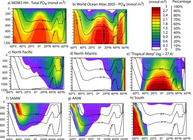
Fig. 8. Zonally-averaged PO3−4 in (a) the HH model and (b) observations. Panels (c–h) show the percentage of total PO3−4 comprised by each regional phosphate tag in the HH model, as labeled at the top of each panel. The colorbar applies to all panels, but is in mmol m−3for panels (a–b) and percentage of total PO3−4 for (c–h).
across the pycnocline. Among the three models with smaller coefficients of vertical mixing, the differences are less stark; still, the SAMW fraction at low latitudes is reduced in the LL model relative to the LL-ECMWF and P2A models, as the latter are forced with stronger Southern Ocean westerly winds (i.e. the ECMWF winds). The water mass fractions obtained from the dye tags and the fraction of low latitude phosphate obtained from the nutrient tags can be quite dif-ferent (Table 3). For example, in the P2A model, the Deep Low latitude tag contributes only 5% of the low latitude py-cnocline waters, but provides 11% of its phosphate, whereas the SAMW-tag contributes 67% of the pycnocline waters but only 48% of the phosphate (Table 3). These differences arise because the phosphate concentration in a tagged water mass may be highly elevated above the phosphate concentration in the pycnocline. Thus, when the water mass is mixed or advected into the pycnocline it can contribute a greater per-centage of the resultant phosphate concentration than the cor-responding contribution of the dye fraction. Such is the case for the phosphate-enriched deep ocean.
Each of the models demonstrates some skill at reproduc-ing the large-scale features of the nutricline: simulated PO3−4 concentrations arch upward from the deep, depleted bowls of
the subtropical gyres to the shallow nutricline of the equator and the high latitudes, just as they do in the observational data (Figs. 8a–b and 9a–b). For brevity, we have chosen to show the zonally-averaged sections only for the HH and P2A models in Figs. 8 and 9; though HH is quite different from the other three models, LL, LL-ECMWF, and P2A are quali-tatively similar, at least as far as the zonally-averaged nutrient sections are concerned.
The Southern Ocean is notable for its elevated near-surface nutrient concentrations (Figs. 8 and 9), which result from strong vertical and lateral advection and mixing of nutri-ents to the surface (Sloyan and Rintoul, 2001; Naveira Gara-bato et al., 2004; Sarmiento et al., 2004) in the presence of weak, iron- and light-limited biological drawdown (Coale et al., 2004). The simplified biogeochemical model from the OCMIP-2 protocol does not simulate an iron cycle, nor does it evaluate the irradiance available for photosynthesis. Nonetheless, the biological model does represent the slug-gish biological PO3−4 drawdown in the Southern Ocean that results from iron and light limitation, because it allows pro-ductivity to remove surface nutrients only when model PO3−4 concentrations exceed observed climatological mean surface PO3−4 concentrations. Because there are high surface PO3−4
a) MOM3 P2A- Total PO4 (mmol m3) b) World Ocean Atlas 2005 - PO4 (mmol m3) 0 200 400 600 800 1000 1200 0 200 400 600 800 1000 1200 0 200 400 600 800 1000 1200 40oS 20oS 0o 20oN 40oN 60oN 60oS 40oS 20oS 0o 20oN 40oN 60oN 60oS 40oS 20oS 0o 20oN 40oN 60oN 60oS 40oS 20oS 0o 20oN 40oN 60oN 60oS 40oS 20oS 0o 20oN 40oN 60oN 60oS 40oS 20oS 0o 20oN 40oN 60oN 60oS 40oS 20oS 0o 20oN 40oN 60oN 60oS 40oS 20oS 0o 20oN 40oN 60oN 60oS
c) North Pacific d) North Atlantic e) “Tropical deep” (σθ > 27.4)
f) SAMW g) AAIW h) South
3 2.7 2.4 2.1 1.8 1.5 1.2 0.9 0.6 0.3 0 100% 90% 80% 70% 60% 50% 40% 30% 20% 10% 0% (mmol m3) Percentage
Fig. 9. Same as Fig. 8, but for the P2A model.
concentrations in the Subantarctic Zone where SAMW is formed, the modeled SAMW is subducted with some of the highest preformed nutrient concentrations in the global pyc-nocline. The high unmodified SAMW phosphate concentra-tions are determined by the OCMIP biogeochemistry, which sets surface nutrients at their climatological values, and is therefore not sensitive to the differing physics in each model. On the other hand, the degree to which these nutrients spread from the SAMW source region to fuel downstream export production is highly dependent on model physics.
This intermodel difference can clearly be seen in tropical nutrient cycling (Figs. 8 and 9). In the HH model compared to the P2A model, the spreading of the SAMW phosphate is restricted to a narrow band near its source region, largely because the high GM coefficient (Ai) creates a parameter-ized southward eddy transport that compensates the north-ward Ekman transport of SAMW (Figs. 8f and 9f). Similarly, this same GM transport causes more restricted spreading of North Pacific phosphate in the HH run relative to the runs with a lower GM coefficient (Figs. 8c and 9c). Furthermore, the deep low latitude phosphate diffuses strongly across the low latitude pycnocline due to the choice of high diapycnal diffusion (Figs. 8e and 9e). This strong diffusion of nutrients across the low-latitude pycnocline also causes the HH model to have lower concentrations of phosphate in the dense
wa-ters underlying the tropics, the highest low-latitude produc-tivity, and the one that disagrees the most with observations (Gnanadesikan et al., 2002).
Winds also affect the extent to which the spreading of the SAMW transports nutrients away from the Southern Ocean (Fig. 10). In the models forced with sluggish Southern Ocean winds (LL and HH), the unmodified SAMW phosphate com-prises the majority of the total pycnocline nutrients only in a narrow band south of 30◦S near the tagging region (Fig. 10) and represents less than 10% of the nutrients in the North-ern Hemisphere gyres. Spreading of the unmodified SAMW phosphate is stronger in the P2A and LL-ECMWF models, contributing up to 20% of the total PO3−4 above the 26.8 isopycnal in the subtropical North Atlantic (Fig. 10, top row). This density horizon is chosen to represent nominally the base of the ventilated pycnocline, but the qualitative results are not sensitive to the density horizon used, as long as it is above the 27.4 isopycnal below which the deep low latitude tag is assigned. Indeed, the relative rank of each tagged phos-phate with regard to its contribution to the low-latitude pyc-nocline phosphate remains the same when averaging above the 27.3 isopycnal as the 26.8 isopycnal.
The importance of SAMW supply is more apparent in the spreading of its remineralized component (Fig. 10, bottom row). Whereas the unmodified SAMW phosphate is largely
b) HH f) HH a) LL e) LL d) P2A c) LL-ECMWF g) LL-ECMWF h) P2A
Fig. 10. The fraction of total phosphate above the 26.8 isopycnal comprised by unmodified SAMW phosphate (top panels) and remineralized
SAMW phosphate (bottom panels) in the 4 models described in Table 2, as labeled at the top of each map. Unmodified SAMW phosphate is phosphate that comes directly from the tagging region without ever fueling productivity, while remineralized SAMW phosphate derives either from DOP tagged in the SAMW source region and remineralized to phosphate or SAMW phosphate that has fueled export production at least once (see Sect. 2.3 for details).
confined to the Southern Ocean, the remineralized SAMW phosphate can propagate far downstream of its tagging re-gion, contributing a significant phosphate source even in the Northern Hemisphere subtropical gyres (Fig. 10). We esti-mate a maximum time scale associated with the conversion of preformed to remineralized SAMW phosphate by divid-ing the total unmodified SAMW phosphate reservoir by the rate of its consumption in fueling primary production. On average across the models, the unmodified SAMW phosphate fuels primary production within 33 years of its creation. The time scale is longest in the P2A model (39 years), which has both a large SAMW unmodified nutrient pool and a weak vertical mixing coefficient outside of the Southern Ocean. The time scale of unmodified SAMW phosphate drawdown is shortest in the HH model (22 years), with its small SAMW pool and higher mixing rates. The designation of unmodi-fied SAMW phosphate is similar to preformed phosphate ex-cept where the nutrients that are tagged outside of the mixed layer. Because the unmodified pool is probably somewhat greater than the preformed pool, these estimates of the time scale for the conversion of SAMW nutrients from preformed to remineralized are likely an upper bound.
3.3 Sustaining low latitude export production
The nutrients tagged in the SAMW region are the most im-portant source of nutrients sustaining low latitude (nominally 30◦S to 30◦N) export production in every model except HH (Fig. 11). In the HH model, productivity throughout the low latitudes is sustained primarily by phosphate that upwells directly from the abyss across the low-latitude pycnocline, and secondarily by the SAMW phosphate. The unmodified phosphate of any variety fuels less than 30% of the total productivity (Fig. 11, right column), and low latitude pro-ductivity draws primarily from the remineralized phosphate pool. Therefore, nutrients reaching the euphotic zone from any source region are utilized at least once, if not many times, before entering a new tagging region. In all models but HH, the unmodified SAMW phosphate sustains more export pro-duction near the equator and in the low latitudes of the North Atlantic than any other unmodified tagged phosphate pool.
Nutrients that cycle through the North Pacific and North Atlantic support relatively little low latitude productivity (Fig. 11). Their most important contribution is in the north-ern half of the subtropical North Atlantic and North Pacific.
1.0 0.8 0.6 0.4 0.2 0 1.0 0.8 0.6 0.4 0.2 0 1.0 0.8 0.6 0.4 0.2 0 1.0 0.8 0.6 0.4 0.2 0 80oS 40oS 0o 40oN 80oN 80oS 40oS 0o 40oN 80oN 80oS 40oS 0o 40oN 80oN 80oS 40oS 0o 40oN 80oN a) LL e) LL-ECMWF c) HH g) P2A Total PO4 Unmodified PO4 20oS 10oS 0o 10oN 20oN 20oS 10oS 0o 10oN 20oN 20oS 10oS 0o 10oN 20oN 20oS 10oS 0o 10oN 20oN 0.3 0.2 0.1 0 0.3 0.2 0.1 0 0.3 0.2 0.1 0 0.3 0.2 0.1 0 b) LL d) HH f) LL-ECMWF h) P2A N. Pacific SAMW N. Atlantic Low-latitude Deep AAIW South
Fig. 11. The zonally-averaged fraction of export production fueled by phosphate (unmodified + remineralized) from each of the tagging
regions (left column) and by the unmodified component of each tagged phosphate between 30◦S and 30◦N (right column) for the four models described in Table 1. Note the panels on the left show the full latitude range of the model ocean, while the panels on the right show only the low-latitudes. The contribution of the remineralized components of tagged phosphate to sustaining low latitude productivity is the difference between the contributions of the total tagged phosphate (left) and the unmodified component of the tagged phosphate (right). Negative values reflect the method used to diagnose the export production fueled by each tagged nutrient using the source/sink terms for DOP and PO3−4 , as described at the end of Sect. 2.3. The lines refer to phosphate from the North Pacific (red solid), North Atlantic (red dotted), Deep low latitude (green solid), SAMW (black solid), AAIW (black dotted), and Southern (magenta solid) regions (refer to Fig. 4 for tagging protocol). Note the different horizontal and vertical scales for the left and right panels.
As the Northern Hemisphere nutrients are advected south-ward of 40◦N, they are promptly consumed and exported. When the sinking flux of the phosphorus penetrates past the 27.4 isopycnal, it is retagged as deep low latitude phosphate, which limits the number of times the northern-tagged phos-phate can fuel productivity via recycling. In addition, a por-tion of the North Atlantic DOP and phosphate sinks with the deep water and spreads to the deep low latitude tagging re-gion (where the North Atlantic tag is reset to zero) without first fueling productivity.
How do nutrients subducted in the SAMW layer at densi-ties greater than those in the subtropical euphotic zone come to influence productivity in low latitudes? To help answer this question, we examine the vertical flux of the SAMW tag
at the depth of the 26.5 isopycnal (Fig. 12), which is regularly ventilated in the subtropical North Atlantic. However, before discussing how the SAMW rises to the shallower isopycnals, we must first address the fact that the tag appears to move downwards at the depth of the 26.5 isopycnal just north of the tagging region. This net downward flux is a consequence of the vertical gradient in SAMW concentrations at the depth of the 26.5 isopycnal just north of the tagging region. In this re-gion, SAMW concentrations decrease with depth across the 26.5 isopycnal because northward transport supplies the tag at the surface while the tagging protocol destroys the tag at depth. The downwelling and vertical diffusion acting on this gradient transport the SAMW tag downward. Downstream of this downwelling domain, the SAMW is transported upwards
20oN 0o 20oS 40oS 40oN 60oS 60oN 20oN 0o 20oS 40oS 40oN 60oS 60oN 50oE 150oE 110oW 10oW 50oE 150oE 110oW 10oW 50oE 150oE 110oW 10oW 50oE 150oE 110oW 10oW
a) HH - Vertical advection b) HH - Vertical diffusion
d) P2A - Vertical advection e) P2A - Vertical diffusion
fraction m-2 s-1 c) HH - Zonal mean vertical flux
20oN 0o 20oS 40oS 40oN 60oS 60oN 20oN 0o 20oS 40oS 40oN 60oS 60oN fraction m-2 s-1
f) P2A - Zonal mean vertical flux
fraction m-2 s-1
-1 0 1
-1 0 1
Fig. 12. Vertical fluxes of SAMW dye (in fractional concentration per m2s) at the depth of the 26.5 isopycnal. Upper row is for the HH model and lower row for P2A. The left hand panels are the vertical advective flux (wC, where w is the vertical velocity and C is the concentration of the SAMW dye tag). The right hand panels are the vertical diffusive flux (κvdC/dz, where κvis the coefficient of diapycnal diffusion). The diffusive flux includes mixing due to convection and stirring due to the GM transport. The colorbar to the right of panel (b) applies to all maps, and positive numbers represent an upwards flux. The line plots are the zonal means of the maps (black for vertical advection and blue for vertical diffusion).
at the depth of the 26.5 isopycnal. The upward transport is primarily achieved by vertical advection in tropical regions, along the eastern fringes of the Southern Hemisphere sub-tropical basins, and in the South Atlantic western boundary current off Brazil (Fig. 12).
Once it has been advected and mixed to shallower depths, the SAMW is transformed by surface buoyancy forcing and diapycnal mixing and may no longer carry the characteris-tic temperature, salinity and potential vorcharacteris-ticity signature it had upon formation and subduction. However, our tags trace the water mass fraction and its nutrients downstream of the tagging regions even as the water mass itself is destroyed by such transformations. The SAMW nutrients that are up-welled into the euphotic zone in the tropics and along the eastern boundaries of the subtropics are consumed and con-verted to organic particles that sink through the water col-umn. These sinking particles are partially remineralized on layers with lighter densities and shallower depths than the SAMW had upon subduction (Toggweiler and Carson, 1995; Williams et al., 2006). Thus, a portion of the nutrients orig-inally subducted in the SAMW remains available to support subtropical productivity as it spreads along these lighter sur-faces to the neighboring subtropical gyres.
Our model results suggest that nutrients slowly lost to depths beneath the pycnocline throughout the low latitudes return to lighter layers primarily in the Southern Ocean. This picture emerges from all models but HH and is summarized in Fig. 13. In the Southern Ocean where biological export does not efficiently compete with the advection and mix-ing of nutrients to the surface layers, nutrients are upwelled and mixed vertically in the ACC and then subducted in the SAMW. Therefore, the water masses formed in the Southern Ocean enter the ocean interior with elevated nutrient concen-trations. Although much of these nutrients are subducted to depths well below the subtropical euphotic zone, their up-welling along the eastern and western fringes of the subtrop-ics and in the tropsubtrop-ics allows these nutrients to sustain sub-tropical export production.
Not far from the SAMW source region, the SAMW unmodified nutrients are consumed and converted to their remineralized counterparts within the pycnocline; further downstream the remineralized nutrients are re-incorporated into organic matter wherever they are mixed and advected into the sunlit surface ocean. In these downstream locales, the slow leakage of organic phosphorus past the base of the seasonally-accessible layers is almost entirely balanced by
0 10 20 30 40 50 60 70 80 Remineralized Unmodified N. Atlantic N. Pacific Low latitude deep (>27.4) SAMW AAIW Southern LL HH LL-ECMWF P2A LL HH LL-ECMWF P2A LL HH LL-ECMWF P2A LL HH LL-ECMWF P2A LL HH LL-ECMWF P2A LL HH LL-ECMWF P2A
Fig. 13. Percentage of low latitude (30◦S–30◦N) export produc-tion fueled by nutrients from different tagged regions, separated by unmodified and remineralized components and by model configura-tion. The salient feature of the graph is that a majority (57–75%) of low latitude productivity is sustained by SAMW nutrients, except in the HH model configuration (33%). Approximately a third of the SAMW nutrients sustaining low latitude productivity are from the unmodified pool, which resemble preformed nutrients when the tags are deployed in the surface mixed layer. Negative values for remineralized tags indicate that unmodified DOP tagged in a given source region is respired to phosphate at a greater rate than the rem-ineralized PO3−4 fuels export production. Such is the case for al-most all of the Southern DOP and much of the North Atlantic DOP.
the lateral and vertical supply of nutrients that were cycled through Southern Ocean water masses. In the HH model, the nutrient budget achieves a slightly more one-dimensional balance: a majority of the sinking flux of nutrients down-ward across the low latitude pycnocline is restored locally via the mixing of nutrients upwards across the low latitude pycnocline. However, even in the HH model, SAMW phos-phate sustains more than a third of low latitude productiv-ity; in the other models the percentage is between 57% and 75% (Fig. 13). Each of the other tagging regions besides SAMW and deep low latitude contributes less than 10% of the phosphate that fuels global low latitude export productiv-ity. There is currently no consensus on where and by what mechanisms the upwelling branch of the MOC is achieved: the distributions of tracers such as δ14C are consistent with
upwelling predominantly in the Southern Ocean (Fig. 7) as are the low coefficients of diapycnal diffusion measured in the ocean interior (Gregg and Sanford, 1980; Ledwell et al., 1993, 1998), while some observationally-based inverse mod-els of overturning suggest a greater role for upwelling at low latitudes (Table 2). This controversy is the motivation for in-cluding 4 different models in this analysis, and the range of our results is thought to span the envelope of likely possibil-ities for the nutrient return pathways occurring in nature.
4 Conclusions, implications, and connections
Our model framework has allowed us to identify the dom-inant nutrient return pathways from the dense ocean inte-rior to depths that are accessible to the sunlit euphotic zone. Between 30◦S and 30◦N, the upper ocean nutrient reser-voir is dominated by those nutrients that were returned from the deep ocean to the pycnocline in the SAMW forma-tion/subduction region of the Southern Ocean (Fig. 13). Only in the model where the coefficient of vertical mixing is set to levels higher than those observed in the pycnocline of the open ocean does mixing directly across the low latitude nu-tricline provide the dominant return pathway of nutrients to the low latitude euphotic zone. The Northern Hemisphere subpolar regions are not the primary suppliers of nutrients to the low latitude euphotic zones; nor are the regions of South-ern Ocean south of the SAMW formation region.
These results are in line with previous modeling studies (Marinov et al., 2006) and with inferences from the distri-bution of tracers such as Si∗(Sarmiento et al., 2004). But there are two major new insights afforded by this study. The first stems from our focus on the sensitivity of nutri-ent pathways to the winds, vertical mixing, and the strength of lateral eddy transport (via changes in the GM coefficient). Our results suggest that in models with high vertical mix-ing, high eddy transport, and low Southern Ocean winds, the dominant nutrient balance is more one-dimensional, i.e. or-ganic nutrients lost by downward sinking at low latitudes are restored through the upward mixing of inorganic nutrients across the pycnocline at these latitudes. At the other extreme, in models with low vertical mixing, weak GM transport, and stronger Southern Ocean winds, organic nutrients lost across the low latitude pycnocline are restored to the pycnocline pri-marily in the Southern Ocean and depend on the full three-dimensional ocean circulation for their delivery to the low latitude euphotic zone.
The second major insight afforded by the study is an ap-proximation of the spatial and temporal scale over which nutrients that enter the ocean interior in the SAMW forma-tion region persist before being utilized in downstream lo-cations. In less than 40 years on average, phosphate enter-ing the ocean interior in the SAMW region is utilized to fuel downstream productivity. In large part, the SAMW nutrients first fuel primary production south of 20◦S. This short spatial
and temporal scale separating the subduction of SAMW nu-trients and their downstream utilization helps explain previ-ous modeling results that tested the influence of the SAMW region on atmospheric carbon concentrations. In the mod-eling study of Marinov et al. (2006), the SAMW nutrient source was “turned off” by forcing nutrients towards zero at the Southern Ocean surface north of the outcropping 27.3 isopycnal, the equivalent of increasing nutrient drawdown by enhanced export production. Although this forced drawdown decimated low latitude productivity by starving these regions of their nutrients, the experiment had little impact on ocean carbon storage or atmospheric carbon concentrations on mil-lenial time scales. The reason for the lack of impact on at-mospheric carbon is that the biological pump had been made much more efficient locally in the SAMW formation region, but the global efficiency was unchanged once the model re-turned to equilibrium (Marinov et al., 2006). In experiments without the forced nutrient drawdown, the SAMW nutrients were already being efficiently consumed downstream of the SAMW formation region on decadal time scales.
Our model experiments suggest a paradigm for returning nutrients to the surface ocean that contextualizes a number of phenomena. For example, it has been hypothesized that biological nitrogen fixation in the North Atlantic is sustained by excess phosphate (phosphate in excess of nitrate relative to their Redfield ratio) advected in the shallow limb of the MOC (Moore et al., 2009). The excess phosphate signature in the shallow MOC layers stems from the SAMW formation region, where high-phosphate waters from the Indo-Pacific Basin are mixed with the water masses advected across the ACC. Iron limits biological nitrogen fixation in the SAMW formation region and throughout the subtropical South At-lantic, so the excess phosphate signature is preserved dur-ing formation and subduction and is exported to the North Atlantic. Because nitrogen fixation in the relatively iron-rich North Atlantic appears to be phosphate-limited (Sa˜nudo-Wilhelmy et al., 2001; Moore et al., 2009), the SAMW ex-cess phosphate source may exert an important control on the rate of nitrogen fixation. Such a dependence implies a cen-tral role for the export of SAMW in the shallow limb of the MOC.
The framework suggested by the modeling experiments also provides a context for results from a recent paleoclima-tology study (Anderson et al., 2009). Anderson et al. (2009) hypothesize that the termination of the last ice age was linked to an increase in Southern Ocean upwelling and the resultant efflux of carbon from the deep ocean to the atmosphere. The primary evidence used to support this hypothesis is the en-hanced burial of biogenic opal in the Southern Ocean and equatorial Pacific, which occurred contemporaneously with the increase in atmospheric CO2and the onset of deglacia-tion. The hypothesized mechanism is an increase in Southern Ocean upwelling, which brings deep carbon to the surface ocean south of the ACC with the upwelling of Circumpolar Deep Water and also advects a pulse of silicic acid across the
ACC into the SAMW formation region. As the carbon out-gases south of the ACC and enters the atmosphere to warm the planet, the silicic acid flux fuels a diatom bloom in the SAMW formation region and – contemporaneously by geo-logical standards – in the equatorial Pacific. The inference from our model experiments that Southern Ocean nutrients fuel a large portion of low latitude productivity and are con-sumed on decadal time scales offers a framework for under-standing this paleo-record.
Having summarized the major insights of our model exper-iments and explored their connections with recent work, we recognize a list of challenges that await future study. First, for a clearer picture of the preformed nutrient content of the interior ocean, it would be helpful to separate nutrients that cycle through the surface mixed layer during water mass for-mation and those that enter water masses via interior mixing and sinking. Second, the MOM3 suite is a set of coarse-resolution models that depend on parameterizations for all mesoscale dynamics and are known to yield qualitatively and quantitatively different results when compared to eddy-resolving models (e.g. Hallberg and Gnanadesikan, 2006). Thus, work with eddy-resolving models should reveal dif-ferent dynamics and possibly lead to difdif-ferent pathways for nutrients. Third, our models are configured with one vertical mixing profile for the global ocean, which was altered only in P2A in order to simulate higher Southern Ocean mixing. Such uniformity in mixing does not capture the observed en-hancement of mixing in regions of rough topography, such as tidal mixing (St. Laurent and Simmons, 2006) which is parameterized in more recent GCMs (Simmons et al., 2004). Finally, the OCMIP-2 biology is not fully prognostic because it is forced towards observations at the surface. Thus, the models cannot represent changes to biology at the surface forced by the models’ differing physics, a challenge that can be tackled with fully prognostic biological models. Future efforts could also move beyond our steady state solution and address temporal variability at time scales other than sea-sonal, incorporate ocean-atmosphere coupling, and examine the hypothesized alterations in the nutrient return pathways under different climate scenarios.
Acknowledgements. The authors are thankful for helpful com-ments from Robbie Toggweiler, Stephanie Downes, Andreas Oschlies, and an anonymous reviewer. The authors acknowl-edge support from the NOAA-Cooperative Institute for Climate Science Grant #NA08OAR4320752; the National Oceanic and Atmospheric Administration, US Department of Commerce award NA07OAR4310096; and the Office of Science (BER), US Depart-ment of Energy, Grant No. DE-FG02-07ER64467. All stateDepart-ments, findings, conclusions, and recommendations are those of the authors and do not necessarily reflect the views of the National Oceanic and Atmospheric Administration, the US Department of Commerce, or the US Department of Energy.