Kinematic and thermal structure at the onset of high-mass star formation

HAL Id: cea-01300597

https://hal-cea.archives-ouvertes.fr/cea-01300597

Submitted on 11 Apr 2016

HAL is a multi-disciplinary open access

archive for the deposit and dissemination of

sci-entific research documents, whether they are

pub-lished or not. The documents may come from

teaching and research institutions in France or

abroad, or from public or private research centers.

L’archive ouverte pluridisciplinaire HAL, est

destinée au dépôt et à la diffusion de documents

scientifiques de niveau recherche, publiés ou non,

émanant des établissements d’enseignement et de

recherche français ou étrangers, des laboratoires

publics ou privés.

Kinematic and thermal structure at the onset of

high-mass star formation

S. Bihr, H. Beuther, H. Linz, S. E. Ragan, M. Hennemann, J. Tackenberg, R.

J. Smith, O. Krause, Th. Henning

To cite this version:

S. Bihr, H. Beuther, H. Linz, S. E. Ragan, M. Hennemann, et al.. Kinematic and thermal structure

at the onset of high-mass star formation. Astronomy and Astrophysics - A&A, EDP Sciences, 2015,

579, pp.A51. �10.1051/0004-6361/201321269�. �cea-01300597�

DOI:10.1051/0004-6361/201321269 c

ESO 2015

Astrophysics

&

Kinematic and thermal structure at the onset of high-mass

star formation

?,??

S. Bihr

, H. Beuther

, H. Linz

, S. E. Ragan

, M. Hennemann

, J. Tackenberg

, R. J. Smith

,

O. Krause

, and Th. Henning

1 _{Max-Planck Institute for Astronomy, Königstuhl 17, 69117 Heidelberg, Germany}

e-mail: name@mpia.de

2 _{Laboratoire AIM, CEA/DSM-CNRS-Université Paris Diderot, IRFU/Service d’Astrophysique, CEA Saclay, 91191 Gif-sur-Yvette,}

France

3 _{Institut für Theoretische Astrophysik, Zentrum für Astronomie, Universität Heidelberg, Albert-Ueberle-Str. 2, 69120 Heidelberg,}

Germany

Received 8 February 2013/ Accepted 18 February 2015

ABSTRACT

Context.Even though high-mass stars are crucial for understanding a diversity of processes within our galaxy and beyond, their formation and initial conditions are still poorly constrained.

Aims.We want to understand the kinematic and thermal properties of young massive gas clumps prior to and at the earliest evolu-tionary stages of high-mass star formation. Do we find signatures of gravitational collapse? Do we find temperature gradients in the vicinity or absence of infrared emission sources? Do we find coherent velocity structures toward the center of the dense and cold gas clumps?

Methods.To determine kinematics and gas temperatures, we used ammonia, because it is known to be a good tracer and thermome-ter of dense gas. We observed the NH3(1, 1) and (2, 2) lines within six very young high-mass star-forming regions comprised of

infrared dark clouds (IRDCs), along with ISO-selected far-infrared emission sources (ISOSS) with the Karl G. Jansky Very Large Array (VLA) and the Effelsberg 100 m Telescope.

Results.The molecular line data allows us to study velocity structures, linewidths, and gas temperatures at high spatial resolution of 3−500

, corresponding to ∼0.05 pc at a typical source distance of 2.5 kpc. We find on average cold gas clumps with temperatures in the range between 10 K and 30 K. The observations do not reveal a clear correlation between infrared emission peaks and ammonia temperature peaks. Several infrared emission sources show ammonia temperature peaks up to 30 K, whereas other infrared emission sources show no enhanced kinetic gas temperature in their surrounding. We report an upper limit for the linewidth of ∼1.3 km s−1_,

at the spectral resolution limit of our VLA observation. This indicates a relatively low level of turbulence on the scale of the obser-vations. Velocity gradients are present in almost all regions with typical velocity differences of 1 to 2 km s−1_{and gradients of 5 to}

10 km s−1_pc−1_{. These velocity gradients are smooth in most cases, but there is one exceptional source (ISOSS23053), for which we}

find several velocity components with a steep velocity gradient toward the clump centers that is larger than 30 km s−1_pc−1_{. This steep}

velocity gradient is consistent with recent models of cloud collapse. Furthermore, we report a spatial correlation of ammonia and cold dust, but we also find decreasing ammonia emission close to infrared emission sources.

Key words.stars: formation – stars: massive – ISM: clouds – ISM: kinematics and dynamics – techniques: interferometric

1. Introduction

Even though the understanding of high-mass star formation has made tremendous progress over the past decade (Beuther et al. 2007;Zinnecker & Yorke 2007;Klessen 2011;Tan et al. 2014), the initial conditions are still poorly constrained. It is known, that stars predominantly form in clusters (Lada & Lada 2003), which is especially true for high-mass stars (e.g., de Wit et al. 2005; Gvaramadze et al. 2012). On observational grounds, the first evolutionary stage of such clusters spawning future high-mass stars might in general be termed pre-protocluster cores (Evans et al. 2002). Their appearance and morphology can be different depending on the environment. Objects of this sort have been

? _{FITS files of Figs. 1 to 6 are only available at the CDS via}

anonymous ftp to cdsarc.u-strasbg.fr (130.79.128.5) or via

http://cdsarc.u-strasbg.fr/viz-bin/qcat?J/A+A/579/A51

??

Appendix A is available in electronic form at

http://www.aanda.org

found in several (sub-)millimeter surveys (e.g.,Klein et al. 2005; Beuther & Sridharan 2007). Also the ISO satellite mission has resulted in a list of such objects revealed by far-infrared obser-vations at 170 µm within the ISO Serendipity Survey (ISOSS, Bogun et al. 1996). For these clumps, cold dust and gas temper-atures have been established in follow-up investigations (Krause et al. 2003,2004). The most prominent variety of young mas-sive clumps are the infrared dark clouds (IRDCs). They were discovered as dark silhouettes against the galactic background at 8 and 15 µm with the Midcourse Space Experiment (MSX, Egan et al. 1998) and ISO (Perault et al. 1996). ISO, MSX, the SpitzerSpace telescope, and further (sub-)millimeter observa-tions have helped for studying these objects in detail (e.g.,Simon et al. 2006;Hennemann et al. 2008;Vasyunina et al. 2009;Ragan et al. 2009;Peretto & Fuller 2009). Because IRDCs can only be seen in absorption against a strong infrared background, their lo-cation is mainly within the disk toward the inner quadrants of our Milky Way, whereas ISOSS sources are more widely distributed.

In fact, the Milky Way midplane had to be avoided for ISOSS because of saturation. IRDCs can have masses up to several thousand solar masses, and the more massive ones are explicitly thought to be progenitors of star clusters (e.g.,Wyrowski 2008; Rathborne et al. 2010;Henning et al. 2010;Ragan et al. 2012a). On average the ISOSS sources have masses less than 500 M (Hennemann et al. 2008). While their masses often are some-what lower than for large high-contrast IRDCs, the general char-acteristics such as low temperature and low turbulent linewidth are similar to IRDCs. Therefore, ISOSS sources are also con-sidered to be early evolutionary stages of intermediate- to high-mass star formation in more isolated regions. Consequently, the better characterization of such clumps (ISOSS and IRDCs) is an important step toward understanding the initial conditions of high-mass star formation.

With the Herschel observatory (Pilbratt et al. 2010), it has been possible to observe the dust content of star-forming re-gions in unprecedented detail at far-infrared wavelengths. To study the onset of star formation, we conducted the Herschel guaranteed time key project – “the earliest phases of star forma-tion” (EPoS). The goal of this project was to map 45 high-mass star-forming regions (Ragan et al. 2012a), as well as 15 low-mass globules (Launhardt et al. 2013) in the far-infrared con-tinuum emission. The sample of 45 high-mass regions includes regions from the subsamples mentioned above: ISOSS sources and IRDCs. An overview of the high-mass regions of the EPoS project is presented in Ragan et al. (2012a). They find al-most 500 point sources within 45 regions and characterize their structure and temperature. More than half of them have 24 µm counterparts. They conclude that the presence of a 24 µm source implies an embedded protostar.

The downside of continuum observations, such as the obser-vations with the Herschel’s bolometer cameras within PACS and SPIRE, is the lack of kinematic information. As the formation process of stars is thought to be highly dynamic (e.g.,Bonnell et al. 2004;Klessen et al. 2005;Csengeri et al. 2011b), such in-formation is crucial for constraining star in-formation theories. As a result, follow-up observations of molecular lines are mandatory for investigating the kinematics of star-forming regions.

Early interferometric measurements toward IRDCs in the (sub-)millimeter range often concentrated on embedded infrared-bright protostars (e.g.,Redman et al. 2003;Pillai et al. 2006b) or in continuum studies that investigate the clump and core fragmentation (e.g., Rathborne et al. 2007). Fewer (sub-)millimeter interferometric studies report on spectroscopic observations. But the interferometric detection of molecular lines (sometimes even CO) away from embedded infrared sources has been difficult (e.g.,Rathborne et al. 2008; Zhang et al. 2009). More recent interferometric studies, with emphasis on investigating the fragmentation of IRDCs, often use N2H+as a tracer (e.g.,Beuther & Henning 2009;Kauffmann et al. 2013; Beuther et al. 2013). However, it is difficult to measure the tem-perature distribution of IRDCs at high angular resultion, since many of the usual temperature tracers in the millimeter, such as CH3CN or H2CO, are problematic when it comes to the low-temperature regime of IRDCs (too low excitation and/or density, freeze-out, etc.). Therefore, measurements of the NH3inversion lines are ideal for temperature maps of IRDC-like environments (Ho & Townes 1983;Ragan et al. 2011;Pillai et al. 2006a).

For this project, we observed ammonia, not just because it is a good thermometer, but it is also known to be a good tracer of dense gas and can be used to study kinematics (Pillai et al. 2006a; Ragan et al. 2012b). As the density of high-mass star-forming regions is in the range 104₋₁₀5 _cm−3

(Beuther et al. 2007), ammonia traces these clumps well. Several ammonia surveys have been conducted recently, using single-dish telescopes with a spatial resolution of >4000 (Pillai et al. 2006a; Dunham et al. 2011;Wienen et al. 2012; Purcell et al. 2012;Chira et al. 2013) and interferometers at high spatial res-olution of <500 _{(Wang et al. 2008; Ragan et al. 2011,2012b;} Devine et al. 2011;Brogan et al. 2011; Zhang & Wang 2011; Lu et al. 2014;Sánchez-Monge et al. 2013). The observed ob-jects vary in terms of mass, distance, evolutionary stages, and infrared emission. The results and conclusions are therefore di-verse. For example,Wang et al.(2008) reports decreasing rota-tional temperature toward the center of the IRDC G28.34+0.06, and the sample ofRagan et al.(2012b) shows active collapse and fragmentation.

Our goal is to resolve the kinematic and temperature struc-ture within a sample of very young high-mass star-forming re-gions at high spatial resolution of ∼3−500, which results in a lin-ear resolution of ∼10 000 AU ≈ 0.05 pc at typical distances of 2.5 kpc. While our target regions are part of IRDC and ISOSS sources, here we concentrate on the substructures within them. To distinguish between clouds, clumps, and cores, we fol-low the nomenclature ofBergin & Tafalla(2007). According to this, cores, clumps, and clouds have sizes of <0.2 pc, 0.3−3 pc, and 2−15 pc, respectively. Similar classifications can be found in the literature (e.g.,Williams et al. 2000;Beuther et al. 2007; Klessen 2011). Clumps are thought to be progenitors of star clus-ters, whereas cores form single or binary stars. Since our ob-jects have sizes between ∼0.3 pc and 1 pc, we classify them as clumps. Within these clumps, we are able to resolve individual cores, which may form single or binary stars. Important ques-tions that we address in this paper are: what is the tempera-ture structempera-ture at the onset of high-mass star formation? Do we see temperature drops toward the highest density peaks simi-lar to low-mass star formation? How dominant is turbulence on the given scale? What are the dynamical signatures of cloud or clump collapse? Can we identify infall signatures on the small scales of individual cores?

In Sect. 2, we explain our observations with the Karl G. Jansky Very Large Array (VLA) and the Effelsberg 100 m Tele-scope. Our observational results are explained in Sect.3, and we discuss them in Sect.4. Section5provides a summary and our conclusions.

2. Observations and data reduction

We observed the NH3(1, 1) and (2, 2) inversion lines of a subset of the EPoS high-mass sample (Ragan et al. 2012a) with the VLA and Effelsberg 100 m Telescopes. The rest frequency of the NH3(1, 1) and (2, 2) inversion lines are 23.694495 GHz and 23.722633 GHz (Ho & Townes 1983), respectively.

2.1. Sample

The observed sample consists of two IRDCs and four ISOSS sources. Their kinematic distances range between ∼1−4 kpc and are taken fromRagan et al.(2012a). They calcu-lated the distance using the method reported inReid et al.(2009). The estimated mass has a wide spread between ∼30 and 800 M (see Sect.3.1). The sample details can be found in Table1and include vlsr, the estimated rms, the synthesized beam size, the distance, the average temperature, the measured SCUBA flux at 850 µm, and the mass estimated from the SCUBA data. We used the SCUBA data to determine the mass (see Sect.3.1).Ragan et al.(2012a) investigated the infrared point sources within the

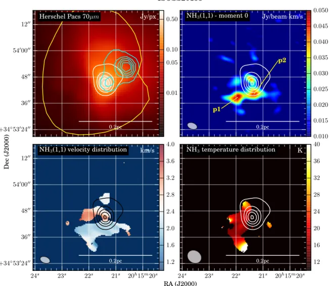
Table 1. Sample details.

Source α (J2000) δ (J2000) vlsr Da rms Beam size hTKi FSCUBA M

name (h:m:s) (◦ :0 :00 ) (km s−1_{) (kpc) (mJy) (}00_×00 ) (K) (Jy) (M) IRDC010.70 18:09:45.9 –19:42:12 +28.8 3.5 ± 0.5 3.0 5.7 × 3.3 b _{6.6 ± 1.3 820}c IRDC079.31 20:31:58.0 +40:18:20 +1.3 1.6+ 2.0_{− 1.6} 3.2 5.1 × 2.9 12.8 5.9 ± 1.2 200 ISOSS18364 18:36:36.0 –02:21:45 +35.0 2.4 ± 0.4 2.9 4.6 × 3.1 12.7 1.4 ± 0.3 110 ISOSS20153 20:15:21.7 +34:53:50 +2.5 1.2 ± 1.1 2.9 4.7 × 2.9 17.0 2.1 ± 0.4 25 ISOSS22478 22:47:49.6 +63:56:45 –39.7 3.2 ± 0.6 3.4 5.0 × 3.0 13.2d _{1.1 ± 0.2 140} ISOSS23053 23:05:22.5 +59:53:50 –51.7 4.3 ± 0.6 3.4 5.1 × 3.1 18.3 4.4 ± 0.9 610

Notes. Source name, coordinates, velocities, distances, rms of line free channels, synthesized beam size, average temperatures from the Effelsberg 100 m Telescope observations, SCUBA-fluxes at 850 µm, and clump masses of our sample.(a)_{Distances are taken fromRagan et al.}

(2012a).(b) _{No Effelsberg data available.}(c)_{Used T = 15 K to calculate mass.}(d)_{Temperature is an upper limit, because of non-detection of}

NH3(2, 2) line.

Table 2. Physical properties of cores.

Source ID α (J2000) δ (J2000) S24 S70 Tdust L M name number (h:m:s) (◦ :0 :00 ) (Jy) (Jy) K L M IRDC079.31 12 20:31:58.3 40:18:38 0.23 1.68 18 25 7 IRDC010.70 10 18:09:45.7 −19:42:08 0.04 2.11 20 98 17 ISOSS18364 2 18:36:36.2 −2:21:49 0.10 14.96 24 173 11 ISOSS20153 1 20:15:21.3 34:53:45 3.32a _{20.83 24 65 4} ISOSS22478 1 22:47:46.6 63:56:49 –b _{0.16 18 10 3} ISOSS22478 2 22:47:46.8 63:56:32 0.10 0.28 21 7 0.8 ISOSS22478 3 22:47:48.2 63:56:44 –b _{0.31 21 9 1} ISOSS22478 4 22:47:50.1 63:56:45 0.11 0.22 20 7 1 ISOSS22478 5 22:47:50.6 63:56:57 –b _{0.27 21 7 0.9} ISOSS23053 2 23:05:21.7 59:53:42 0.10 7.63 21 441 56 ISOSS23053 3 23:05:23.7 59:53:53 0.51 18.16 22 869 84

Notes. Core properties investigated byRagan et al.(2012a). The ID number describes the core number of each clump specified inRagan et al.

(2012a). S24is Spitzer MIPS 24 µm and S70is Herschel PACS 70. Temperature, mass, and luminosity are calculated from a best-fit spectral energy

distribution of the Herschel infrared data using the PACS 70, 100, 160 µm data. Details can be found inRagan et al.(2012a).(a)_{IRAS 25 µm flux.} (b)_{Not detected.}

EPoS sample. Our sample includes some of these cores, and their details are given in Table2.

2.2. Very Large Array observations

The VLA observations were conducted in July and August 2010 during the VLA upgrade as shared risk observations. We used the array in D configuration, achieving a synthesized beam of 3−500_{. As a flux and bandpass calibrator, we} ob-served J1331+3030 and J1733-1304, respectively. Phase cali-brations were done with regular observations of J2025+3343, J2322+5057, J1743-0350, and J1851+0035 every ∼5 min and pointing every ∼30 min.

Because the WIDAR correlator was used to observe the NH3(1, 1) and (2, 2) lines simultaneously, we could avoid most relative calibration errors. A bandwidth of 4 MHz and 64 chan-nels resulted in a channel width of 62.5 kHz. This corresponds to a spectral resolution of ∼0.8 km s−1. The bandwidth of 4 MHz gives us a velocity range of ∼50 km s−1_{. The low sensitivity of} the edge channels meant that we are not able to use ∼5%−10% of the edge channels. We therefore can use about 55 channels for our analysis, which gives us a velocity range of ∼44 km s−1. This allows us to observe both the inner satellite and one outer satel-lite of the NH3(1, 1) hyperfine structure (see Figs.A.1–A.6). To achieve a 1σ noise level of ∼3 mJy beam−1, we integrated 30 min per source.

The VLA data were calibrated, reduced, and cleaned with the CASA 3.3 package (Common Astronomy Software Applications), provided by NRAO.

2.3. Effelsberg 100 m Telescope observations

To overcome missing-flux problems and to reconstruct large scale structures, we observed our sample with the Effelsberg 100 m Telescope in January and February 2012 (ex-cept IRDC010.70 since it is not ideal to observe with the Effelsberg 100 m Telescope owing to low declination). We ob-served raster maps in frequency-switching mode, covering the whole VLA primary beam of ∼12000. The primary beam of Effelsberg at 1.3 cm is 4000_{, and with an approximate} Nyquist-sampling of ∼2000, this requires map sizes of 7 × 7 positions. For the smaller objects in our sample (ISOSS18364, ISOSS20153), we observed 5 × 5 positions. We used the new fast Fourier transform spectrometer (×FFTS) with a bandpass of 100 MHz and 32 768 channels, centered at 23 708.5646 MHz. This setup allowed us to observe the NH3 (1, 1) and (2, 2) lines (includ-ing the full hyperfine structure) simultaneously, hence to elimi-nate most relative calibration errors. The spectral resolution was ∼0.04 km s−1_{. As a flux calibrator, we used NGC 7027 (Zijlstra} et al. 2008).

With an integration time of 4 min per raster position, we achieved a 1σ noise level of ∼20−70 mJy beam−1, dependent on the declination of the source, multiple coverage, and weather conditions. The data calibration and imaging was done with GREG and CLASS of the GILDAS package by IRAM.

2.4. Combination of single-dish and interferometry data We used the feather task in CASA to combine the VLA and Effelsberg 100 m Telescope data. The Effelsberg 100 m

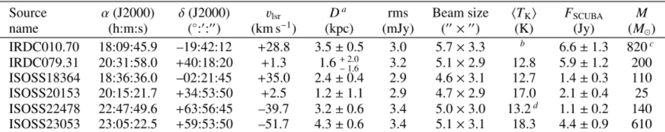
Fig. 1.IRDC010.70 – overview. Upper left panel: Herschel PACS 70 µm emission and cyan contours present Spitzer MIPS 24 µm emission at levels of 90, 110, 130, and 150 MJy/sr. The yellow contour shows the 3-sigma limit of the SCUBA 850 µm emission and therefore the area where we measured the clump mass. Following panels: VLA data. Upper right panel: integrated emission of the main NH3(1, 1) line in Jy beam−1km s−1

from 27.1 to 30.3 km s−1_{. Lower left panel: peak velocity distribution in km s}−1_{. Lower right panel: kinetic temperature in K. We extracted the}

temperature distribution along the black and white lines shown in the lower right panel and plotted the values as a function of distance in Fig.10. In each panel contours present Herschel PACS 70 µm emission at levels of 2.5, 5, 7.5, and 10 mJy/px for white/black contours and 20, 30, 40, and 50 mJy/px for gray contours. The NH3(1, 1) emission peak is marked in the upper right panel, and the corresponding spectra are given in Fig.A.1.

The synthesized beam and scale are shown in each panel.

Telescope data had to be smoothed to the spectral reso-lution of the VLA (∼0.8 km s−1_{). The combined data} in-cludes the large scale structure (∼4000) observed with the Effelsberg 100 m Telescope, as well as the small scale struc-ture (∼3−500) observed with the VLA. The missing flux in the VLA data depends on the source structure, sidelobes, and inte-gration area and ranges between ∼40–95%.

3. Results

Figures1to6show the Herschel PACS 70 µm image for each source in the upper lefthand panel, the integrated NH3(1, 1) emission of the main hyperfine component in the upper right-hand corner, the peak velocity distribution in the lower leftright-hand panel, and the temperature distribution in the lower righthand corner.

3.1. Clump masses

We used the SCUBA 850 µm data (Di Francesco et al. 2008) to determine clump masses. These data have a beam size of 22.900 and an absolute flux uncertainty of 20%. The measured flux is used to calculate the clump mass, assuming optically thin dust emission:

Mgas=d

2_FνRgas

Bν(T ) κ , (1)

where d is the distance of the clump, Fν the flux density, Rgas the gas-to-dust mass ratio, Bν(T ) the Planck function at tem-perature T (estimated from the NH3observations, see Sect.3.3 and Table1), and κ the dust-mass absorption coefficient. We as-sumed a gas-to-dust mass ratio of 100. To determine κ, we used the dust model ofOssenkopf & Henning(1994) with a density of 105 _cm−3 _{with thin ice mantles and interpolated to 850 µm,}

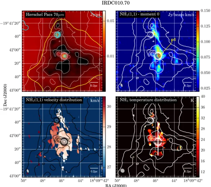
Fig. 2.IRDC079.31 – overview. Upper left panel: Herschel PACS 70 µm emission and black contours present Spitzer MIPS 24 µm emission at levels of 80, 115, and 150 MJy/sr. The yellow contour shows the 3-sigma limit of the SCUBA 850 µm emission and therefore the area where we measured the clump mass. Following panels: VLA and Effelsberg 100 m Telescope data combined. Upper right panel: integrated emission of the main NH3(1, 1) line in Jy beam−1km s−1from −0.3 to 2.8 km s−1. Lower left panel: peak velocity distribution in km s−1. Lower right panel:

kinetic temperature in K. We extracted the temperature distribution along the black line shown in the lower right panel and plotted the values as a function of distance in Fig.10. In each panel contours present Herschel PACS 70 µm emission at levels of 4, 8, 12, 16, and 20 mJy/px for

white/black contours and 30, 50, 70, 90, and 110 mJy/px for gray contours. The NH3(1, 1) emission peaks are marked in the upper right panel,

and the corresponding spectra are given in Fig.A.2. The synthesized beam and scale are shown in each panel.

which results in κ = 1.5 cm2g−1. The temperature was taken from the Effelsberg 100 m Telescope NH3observations because these observations give an average value for the temperature. We chose a 3σ limit as the boundary for the SCUBA flux measure-ments (213 mJy beam−1_{and 229 mJy beam}−1_{for the} fundamen-tal and extended maps, respectivelyDi Francesco et al. 2008).

The uncertainties in distance (see Table 1) and tempera-ture are difficult to estimate, and we assume an uncertainty of ∼20%. Different dust models could be applied (thin or thick ice mantles), and this could change κ by ∼20%. Di Francesco et al.(2008) reports an absolute flux uncertainty of 20% for the SCUBA 850 µm data. A different gas-to-dust ratio could also change the mass. Taking all these individual uncertainties into account reveals an uncertainty in mass of a factor of ∼4 to 5.

Our sample shows a wide spread in clump masses, and the values are given in Table 1. The masses given in Table 2 are

lower, since these masses only describe the core masses of the infrared sources, but not the entire clump.

3.2. Kinematics

Our limited spectral resolution with the VLA of 0.8 km s−1 pro-hibits us from resolving very narrow lines. In cases where the line falls within one spectral channel, the CLASS fitting algo-rithm gives an upper limit for the FWHM of 1.3 km s−1. Several sources in our sample show linewidths that are broader than our resolution limit (e.g., ISOSS23053, ISOSS20153, IRDC079.31), but except for ISOSS20153, further analysis and comparison with the Effelsberg 100 m data, which has a high spectral res-olution, identified this linewidth broadening as a superposition of several narrow lines that are slightly shifted. The steep veloc-ity gradient within ISOSS23053 is the most prominent example of such a linewidth superposition (see Sect.4.1.3). ISOSS20153

220₀₀00 5000 4000 3000 −2◦₂₁0₂₀00 Jy/px Herschel Pacs 70µm 0.2pc 0.01 0.05 0.10 0.50 Jy/beam·km/s NH3(1,1) - moment 0 0.2pc 0.01 0.02 0.03 18h₃₆m₃₅s 36s 37s 220₀₀00 5000 4000 3000 −2◦₂₁0₂₀00 km/s NH3(1,1) velocity distribution 0.2pc 34.0 34.5 35.0 35.5 36.0 18h₃₆m₃₅s 36s 37s K NH3temperature distribution 0.2pc 12 16 20 24 28 32 36 40 RA (J2000) Dec (J2000) ISOSS18364 p1

Fig. 3.ISOSS18364 – overview. Upper left panel: Herschel PACS 70 µm emission. The yellow contour shows the 3-sigma limit of the SCUBA 850 µm emission and therefore the area where we measured the clump mass. Following panels: VLA and Effelsberg 100 m Telescope data combined. Upper right panel: integrated emission of the main NH3(1, 1) line in Jy beam−1km s−1from 34.2 to 36.6 km s−1. Lower left panel: peak

velocity distribution in km s−1_{. Lower right panel: kinetic temperature in K. We extracted the temperature distribution along the black line shown}

in the lower right panel and plotted the values as a function of distance in Fig.10. In each panel white/black contours present Herschel PACS 70 µm emission at levels of 15, 30, 50, 100, 200, and 300 mJy/px and cyan contours present PdBI continuum 3.4 mm at levels of 0.4, 0.8, 1.2, 1.6, and 2 mJy/beam with a synthesized beam of 4.600

× 3.200

(Hennemann et al. 2009). The NH3(1, 1) emission peak is marked in the upper right

panel, and the corresponding spectra are given in Fig.A.3. The synthesized beam and scale are shown in each panel.

is the only source in which the FWHM broadens to ∼2.5 km s−1 at the position of an infrared point source. Otherwise, from the combined data, most clouds exhibit linewidths at the upper limit of 1.3 km s−1_{. On the other hand, the high spectral resolution,} but low spatial resolution of our Effelsberg 100 m Telescope ob-servations indicate an average linewidth for each clump of 1.1 to 1.7 km s−1.

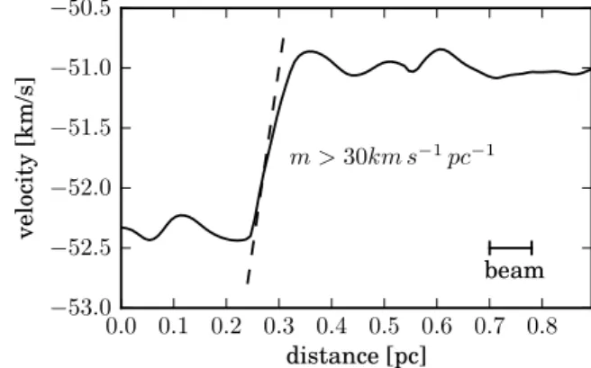
With the exception of ISOSS23053, the clumps reveal a smooth peak velocity structure with amplitudes of 1 to 2 km s−1 and projected linear gradients of 5 to 10 km s−1pc−1. In contrast to this, ISOSS23053 reveals two separate velocity components (see Fig.6) with a difference of ∼1.5 km s−1, but minor veloc-ity fluctuations within each component. The sharp velocveloc-ity step, situated between the two components, is unique in our sample. Figure 7shows a position-velocity cut that is perpendicular to the velocity step, where the velocity gradient increases to at least 30 km s−1pc−1. We discuss the kinematics in general and explore the interpretations of the steep velocity step in Sect.4.1.

3.3. Temperature

To calculate temperature maps, we used the method described in Ho & Townes(1983).Ragan et al.(2011) also provides a com-prehensive summary of this method. A 3σ limit of the NH3(1, 1) and (2, 2) emission were used for trustworthy results, whereas the NH3(2, 2) emission was mainly limiting the area of our tem-perature maps. To increase the area of reliable NH3(2, 2) emis-sion, we used a uvtaper of 30 kλ, which implies giving less weight to long baselines. This method increases the signal-to-noise ratio, but also increases the synthesized beam to 5−700_.

Between 5 K and 25 K, the rotation temperature derived from the NH3(1, 1) and (2, 2) lines can be converted into kinetic tem-peratures well (Danby et al. 1988;Tafalla et al. 2004). However, above 25 K, these low-level NH3 lines are no longer sensitive to the actual kinetic temperature, so higher temperatures have to be treated with care. In the following, we talk about the kinetic temperature.

+34◦₅₃0₂₄00 3600 4800 540₀₀00

1200 Herschel Pacs 70µm Jy/px

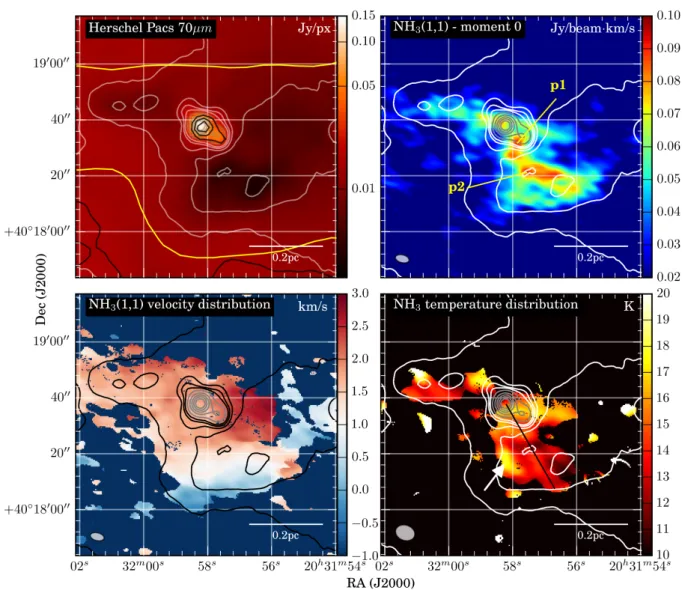
0.2pc 0.01 0.05 0.10 0.50 NH3(1,1) - moment 0 Jy/beam·km/s 0.2pc 0.010 0.015 0.020 0.025 0.030 0.035 0.040 0.045 0.050 20h₁₅m₂₀s 21s 22s 23s 24s +34◦₅₃0₂₄00 3600 4800 540₀₀00 1200 NH3(1,1) velocity distribution km/s 0.2pc 1.2 1.6 2.0 2.4 2.8 3.2 3.6 4.0 20h₁₅m₂₀s 21s 22s 23s 24s K NH3temperature distribution 0.2pc 12 16 20 24 28 32 36 40 RA (J2000) Dec (J2000) ISOSS20153 p1 p2

Fig. 4.ISOSS20153 – overview. Upper left panel: Herschel PACS 70 µm emission and cyan contours present Spitzer MIPS 24 µm emission at levels of 150, 250, 350, 450, and 550 MJy/sr. The yellow contour shows the 3-sigma limit of the SCUBA 850 µm emission and therefore the area where we measured the clump mass. Following panels: VLA and Effelsberg 100 m Telescope data combined. Upper right panel: integrated emission of the main NH3(1, 1) line in Jy beam−1km s−1from 0.8 to 4.0 km s−1. Lower left panel: peak velocity distribution in km s−1. Lower

right panel: kinetic temperature in K. In each panel white/black contours present Herschel PACS 70 µm emission at levels of 0.1, 0.2, 0.3, 0.4, and 0.5 Jy/pixel. The NH3(1, 1) emission peaks are marked in the upper right panel, and the corresponding spectra are given in Fig.A.4. The

synthesized beam and scale are shown in each panel.

The observed kinetic temperatures within our sample range from 10−30 K and show a clumpy structure down to the resolution limit. Several sources (e.g., IRDC079.31, ISOSS23053 SMM2) show signs of increasing temperatures of 20−30 K toward infrared emission sources (see Sect. 4.3 for further details). On the other hand, several sources (e.g., ISOSS20153) show marginal ammonia emission close to in-frared emission sources (see Sect.4.2), making it impossible to measure the temperature in these regions.

4. Discussion

The discussion is divided in three parts. First we discuss the kinematical structure of our sample and look for signs of col-lapse. The second part is devoted to the morphological structure of the ammonia emission and a comparison to infrared emission. Finally we discuss the temperature structure and search for ex-ternal or inex-ternal heating sources.

4.1. Kinematical structure

Infrared dark clouds exhibit significant non-thermal linewidths, even though high-resolution observations suggest that IR-dark regions are relatively more quiescent than the surrounding gas (e.g.,Pineda et al. 2010;Hernandez et al. 2012). Therefore we expect a linewidth larger than ∼0.3 km s−1 _{for our observations} (thermal linewidth), but smaller than ∼2 km s−1(quiescent inte-rior of IRDCs). As explained in Sect.3.2, our observations are limited to an upper limit of 1.3 km s−1for the linewidth, and most of our sources show this upper limit. In this section we explore what the dynamics of our gas clumps tell us about the onset of high-mass star formation.

4.1.1. Virial parameter

As outlined in Sect. 3.2, the Effelsberg 100 m data allow us to determine the spatially averaged linewidths of our clumps.

+63◦₅₆0₁₅00 3000 4500 570₀₀00

1500 Herschel Pacs 70µm Jy/px

1 2 3 4 5 0.2pc 0.005 0.010 0.020 Jy/beam·km/s NH3(1,1) - moment 0 0.2pc 0.01 0.02 0.03 0.04 0.05 22h₄₇m₄₆s 48s 50s 52s 54s +63◦₅₆0₁₅00 3000 4500 570₀₀00 1500 NH3(1,1) velocity distribution km/s 0.2pc −39 −40 −41 −42 22h₄₇m₄₆s 48s 50s 52s 54s K NH3temperature distribution 0.2pc ₁₂ 16 20 24 28 32 36 40 RA (J2000) Dec (J2000) ISOSS22478 p1

Fig. 5.ISOSS22478 – overview. Upper left panel: Herschel PACS 70 µm emission, and cyan contours present Spitzer MIPS 24 µm emission at levels of 15, 40, 65, 90, and 115 MJy/sr. The yellow contour shows the 3-sigma limit of the SCUBA 850 µm emission and therefore the area where we measured the clump mass. The numbers are the core numbers of Table2. Following panels: VLA and Effelsberg 100 m Telescope data

combined. Upper right panel: integrated emission of the main NH3(1, 1) line in Jy beam−1km s−1from −41.3 to −38.9 km s−1. Lower left panel:

peak velocity distribution in km s−1_{. Lower right panel: kinetic temperature in K. In each panel white/black contours present Herschel PACS 70 µm}

emission at levels of 3, 4.5, 6, and 7.5 mJy/pixel. The NH3(1, 1) emission peak is marked in the upper right panel, and the corresponding spectra

are given in Fig.A.5. The synthesized beam and scale are shown in each panel.

These linewidths are used to calculate virial masses following MacLaren et al.(1988):

Mvirial= k2R∆v2, (2)

where M is the mass in M, R the radius in pc, and∆v the ve-locity FWHM in km s−1. The factor k2 depends on the density profile and has values of k2= 210 for ρ = constant, k2= 190 for ρ ∝ 1/r and k2= 126 for ρ ∝ 1/r2_{(MacLaren et al. 1988). The} virial parameter is defined as

α = Mvirial

Mgas · (3)

The gas mass is determined by the continuum data at 850 µm (see Sect.3.1for details). We choose a circle of 4000 diameter around the peak position given in Table1, which corresponds to the Effelsberg 100 m Telescope beam. Table3presents the virial mass, the linear diameter of the 4000circle, the gas mass and the virial parameter. The gas masses used here are lower than those

given in Table1, since we only consider the central area of the clump in order to obtain a consistent comparison between the virial and gas mass.

As explained in Sect. 3.1, the calculated gas masses have an uncertainty of a factor of 4−5. The uncertainty for the virial masses is smaller with a factor of 2−3 and is mainly due to the uncertainty in the distance estimate and the density profile. Another uncertainty is the assumption that the gas mass Mgas, measured via the dust emission at 850 µm, and the virial mass Mvirial, measured via the line width of the NH3(1, 1) transi-tion, trace the same gas. However, the spatial structure of the Effelsberg 100 m NH3(1, 1) observations is similar to the 850 µm emission, which implies that the assumption is reasonable.

The virial parameter is an indicator of gravitational stability, because values lower than one indicate gravitational collapse, whereas values over one are consistent with the regions not being bound. Virial parameters close to one indicate a balance between gravity and thermal or turbulent motions. In this simple analysis,

+59◦₅₃0₃₀00 4500 540₀₀00 1500 Jy/px SMM2 SMM1 Herschel Pacs 70µm 0.2pc 0.01 0.05 0.10 0.50 Jy/beam·km/s NH3(1,1) - moment 0 0.2pc 0.02 0.04 0.06 0.08 0.10 0.12 23h₀₅m₁₈s 20s 22s 24s 26s +59◦₅₃0₃₀00 4500 540₀₀00 1500 km/s NH3(1,1) velocity distribution 0.2pc −53 −52 −51 23h₀₅m₁₈s 20s 22s 24s 26s K NH3temperature distribution 0.2pc 12 16 20 24 RA (J2000) Dec (J2000) ISOSS23053 p1 p2

Fig. 6.ISOSS23053 – overview. Upper left panel: Herschel PACS 70 µm emission, and cyan contours present Spitzer MIPS 24 µm emission at levels of 75, 150, 225, and 300 MJy/sr. The yellow contour shows the 3-sigma limit of the SCUBA 850 µm emission and therefore the area where we measured the clump mass. Following panels: VLA and Effelsberg 100 m Telescope data combined. Upper right panel: integrated emission of the main NH3(1, 1) line in Jy beam−1km s−1 from −53.3 to −50.1 km s−1. Lower left panel: peak velocity distribution in km s−1, and the black

line indicates the direction of the position-velocity cut shown in Fig.7. Lower right panel: kinetic temperature in K. We extracted the temperature distribution along the black line shown in the lower right panel and plotted the values as a function of distance in Fig.10. The black circles indicate SpitzerMIPS 24 µm emission sources. In each panel white/black contours present Herschel PACS 70 µm emission at levels of 20, 40, 60, 100, 200, 300, and 400 mJy/pixel. The NH3(1, 1) emission peaks are marked in the upper right panel, and the corresponding spectra are given in Fig.A.6.

The synthesized beam and scale are shown in each panel.

we do not consider additional aspects, such as magnetic fields or external pressure. Our sample has virial parameters between 0.4 and 4.0 with a mean of 1.6. Considering the uncertainties in the masses, we report that the sample as a whole is consistent with an approximate virial balance. This result is consistent with a recent ammonia survey of IRDCs byChira et al. (2013). They observed 110 IRDCs with the Effelsberg 100 m Telescope and found an average virial parameter around one. Similar results have been found by Wienen et al. (2012) and Dunham et al. (2011). However, our sample does contain individual clumps that have virial parameters clearly in excess of unity, or below it. ISOSS23053 is extremely massive and has an estimated virial parameter of 0.4−0.6. This is suggestive of a clump undergo-ing large scale collapse, as we discuss in Sect. 4.1.4. In con-trast, ISSOSS2015 has the lowest gas mass in the sample, and even at the upper end of our uncertainty estimate it can only be marginally bound.

4.1.2. Rotational energy

As outlined in Sect.3.2, several of our clumps have smooth ve-locity gradients, which could be due to rotation of the clump. By assuming solid-body rotation of a sphere with uniform den-sity, we can estimate the rotational energy and compare it with the gravitational energy, using the beta parameter (Stahler et al. 2005):

β = Erot Egrav

=Ω2cos(i)2R3

3 G M , (4)

whereΩ is the angular velocity, R the radius of the clump, G the gravitational constant, and M the mass of the rotating clump. The angular velocity depends on the inclination, which we define to be zero if the angular rotation is perpendicular to the line of sight. As we cannot determine the inclination with our observa-tions, we assume it is edge-on (i= 0◦_{). We focus our analysis on}

Table 3. Virial analysis.

Object ∆v Linear diameter Mgas. Mvir(ρ ∝ 1/r) Mvir(ρ ∝ 1/r2) α (ρ ∝ 1/r) α (ρ ∝ 1/r2)

[km s−1_{] [pc] [M} ] [M] [M] IRDC079.31 1.7 0.3 70 180 120 2.4 1.6 ISOSS18364 1.1 0.5 90 110 75 1.2 0.8 ISOSS20153 1.3 0.2 20 80 50 4.0 2.6 ISOSS22478 1.1 0.6 100 150 100 1.5 1.0 ISOSS23053 1.2 0.8 370 230 150 0.6 0.4

Notes. The masses are measured within a circle of 4000

diameter around the peak position given in Table1. The corresponding linear diameter is given.∆v is measured for the peak spectrum observed with the Effelsberg 100 m Telescope. Virial masses and virial parameter are given, depending on the density profile of the clump. For ISOSS23053, we chose the linewidth of the red component (see Sect.4.1.3).

IRDC079.31 and ISOSS18364, as these show a smooth velocity gradient over the entire clump. The corresponding gradients are ∼10 km s−1pc−1and ∼6 km s−1pc−1, for both sources in north-south direction. Once again we use the area corresponding to the Effelsberg beam as in the virial analysis. For these regions, the value of beta are β = 0.37 and β = 0.48 for IRDC079.31 and ISOSS18364, respectively. Assuming a more realistic den-sity profile of ρ ∝ 1/r2_{reduces β by a factor of 3 (Ragan et al.} 2012b). The uncertainty of β is within the same order of magni-tude as the uncertainty in the mass measurement and therefore a factor of ∼4−5.

Previous studies have indicated that the rotational energy does not contribute significantly to the overall energy budget of the clumps. For example,Goodman et al.(1993) found values of beta ∼0.02 for cores with size ∼0.1 pc. For a homogeneous com-parison with our data, we recalculated the β values for the IRDCs studied inRagan et al.(2012b). They report velocity gradients of ∼2 km s−1pc−1for the IRDCs G005.85-0.23 and G024.05-0.22. The corresponding radii and masses (R ∼ 0.25 pc and 0.6 pc, M ∼ 500 M and 2500 M, respectively) result in β values of 0.01 and 0.03, which are similar to those reported inGoodman et al.(1993). The β values in our study are a factor of 10 larger.

Our measurements are close to the breakup speed of spher-ical clumps, which corresponds to β values greater than 1/3 (Stahler et al. 2005). This is even true if we consider the uncer-tainties and use a more realistic centrally peaked density profile. This implies that for our sources, the assumption of circular solid body rotation is a poor description of our data. The observed ve-locity gradient might instead have a different origin, such as gas flows toward the center. Such flows might also be consistent with the steep velocity steps that we see in the observations.

4.1.3. Steep velocity step within ISOSS23053

ISOSS23053 is known to be an active star-forming region (Birkmann et al. 2007; Pitann et al. 2011). Multiwavelength observations reveal several protostar candidates, outflows, and signs of infall. Submillimeter observations disclose a gas reser-voir of several hundred solar masses (Birkmann et al. 2007). However, no previous observations have resolved the kinematic structure spatially.

ISOSS23053 harbors two velocity components at

−52.5 km s−1 _{and −51 km s}−1_{. A spatially unresolved} ve-locity step is found between these components, which has a gradient larger than 30 km s−1 _pc−1_{. The velocity step follows} the 24 µm and 70 µm emission from northeast to southwest (see lower left panel in Fig.6). Figure7shows the position velocity cut along the axis marked in Fig.6.

0.0 0.1 0.2 0.3 0.4 0.5 0.6 0.7 0.8 distance [pc] −53.0 −52.5 −52.0 −51.5 −51.0 −50.5 velocity [km/s] beam m > 30km s−1_pc−1

Fig. 7.Position velocity cut of ISOSS23053 along the black line indi-cated in the lower-left panel of Fig.6.

Fig. 8. Central spectra of ISOSS23053, as observed with the Effelsberg 100 m Telescope. The green curve represents one component fit, the blue and red curves represent a two-component fit.

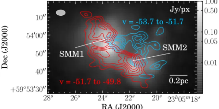
The Effelsberg 100 m Telescope observations help to de-fine the two velocity components accurately, thanks to their higher spectral resolution (see Fig. 8). The first component has a velocity range from −53.7 to −51.7 km s−1 _{(the “blue} component”), and the second component is from −51.7 to −49.8 km s−1 (the “red component”). Figure 9 shows the NH3 (1, 1) emission for both components separately. The com-ponents overlap at two positions, which are close to SMM1 and SMM2, respectively. The overlap close to SMM1 (northeast) falls within one beam and is therefore not resolved, whereas the second overlap close to SMM2 (southwest) is broader. The Effelsberg 100 m Telescope observations reveal an average linewidth for each component of ∼1.2 km s−1(blue component) and ∼0.9 km−1_{(red component), as illustrated in Fig.8.}

23h₀₅m₁₈s 20s 22s 24s 26s 28s RA (J2000) +59◦₅₃0₃₀00 4000 5000 540₀₀00 1000 Dec (J2000) Jy/px v = -53.7 to -51.7 v = -51.7 to -49.8 SMM2 SMM1 0.2pc 0.01 0.05 0.10 0.50 1.00

Fig. 9. ISOSS23053 – velocity structure. The gray-scale represents Herschel PACS 70 µm. The red and blue contours represent the NH3 (1, 1) moment 0 of each component at levels of 30, 40, 50, 60,

70, and 80 mJy beam−1_{km s}−1_.

The origin of the velocity step observed in ISOSS23053 is challenging to explain. Because the optical depth is low (τ < 0.7), we cannot explain this structure via self absorption of the two components. In the following we propose a solution.

The observations reveal several velocity components along the line of sight. However, the question is whether these com-ponents are spatially connected and/or interact with each other. Figure 9 shows the ammonia emission of both velocity com-ponents separately. The three-dimensional shape of this clump could be a filamentary structure along the line of sight, at which SMM1 shows the beginning and end of the filament, whereas SMM2 is the connection in between. In this picture, the two components at SMM1 could be spatially unconnected. On the other hand, it could also be that the two velocity components at SMM1 and SMM2 are spatially connected and that the velocity structure stems from the dynamical collapse of converging gas flows.

This velocity structure is also reported for other sources; for example, Csengeri et al. (2011a,b) report similar velocity steps for DR21(OH). They observed N2H+ with the PdBI and find a velocity shear close to the center, but slightly offset from the strong continuum sources. Their interpretation is that there are converging gas flows toward the central gravitational well. Beuther et al. (2013) also find multiple velocity components in the starless high-mass star-forming region IRDC 18310-4, which are consistent with collapse motions. Recently, Smith et al. (2013) have modeled the velocity structure in dynami-cally collapsing gas clumps, and they find similar steep velocity gradients close to the clump centers with velocity gradients up to 20 km s−1pc−1. Therefore, ISOSS23053 might undergo global dynamical collapse, and this would explain the active star forma-tion along the velocity step.

4.1.4. Signature of collapse?

To summarize, we find one example in our sample

(ISOSS23053) with a steep velocity gradient that might represent ongoing gravitational collapse. In addition we find in two sources (IRDC079.31 and ISOSS18364) smooth velocity gradients, which are poorly described by solid-body rotation and may indicate gas flows toward the clump center. The three other clumps in our sample show no clear evidence of gravitational collapse.

After combining these results with recent findings in other sources (e.g., Csengeri et al. 2011a,b; Schneider et al. 2010; Beuther et al. 2012), this indicates that large-scale gravitational

collapse might be present in several regions of young massive star formation. However, we have not identified any unambigu-ous signatures yet.

4.2. Ammonia morphology and correlation with gas and dust Ammonia is a good tracer of cold dense gas (e.g.,Ho & Townes 1983;Pillai et al. 2006a;Tafalla et al. 2004;Ragan et al. 2011), but how might this correlation change in the presence of embed-ded infrared emission sources? Complementary Herschel and Spitzerdata allow us to investigate possible deviations from the close correlation between ammonia and submillimeter emission, which indicates dense gas.

ISOSS18364 is a clear example of a case where ammo-nia and submillimeter emission are very closely coupled only in infrared-dark regions. TheHennemann et al. (2009) 3.2 mm PdBI data show that this IRDC breaks into a north and a south clump (see cyan contours in Fig.3). No infrared sources are ev-ident to the north, and the ammonia peak is consistent with the 3.2 mm peak. The southern peak is the site of 24 and 70 µm emis-sion, and ammonia does not match the submillimeter emission. This trend is seen consistently throughout the sample. Positions with strong 24 µm emission have little to no ammonia emission (except ISOSS22478 peak 4). On the other hand, positions with strong 70 µm emission and little or no 24 µm emission do show coincident ammonia emission.

This observation of decreasing ammonia emission with in-creasing 24 µm flux is surprising, because other ammonia obser-vations in the literature of similar objects at similar resolutions show a good correlation between 24 µm emission peaks and am-monia emission peaks (Devine et al. 2011;Ragan et al. 2012b).

While we do not have a conclusive explanation for this observation, we do suggest two possibilities in the following. The chemistry of ammonia is complicated, and different mod-els show contradictory results.Millar et al.(1997) claims that a low ammonia abundance can be explained by depletion, mean-ing that ammonia freezes out on grain mantles. More recently, Vasyunina et al.(2012) have reported similar results. They show that the ammonia abundance drops for chemical models that consider gas-grain networks and find that ammonia depletes on grains at typical IRDC conditions (T = 15 K, n = 105 _cm−3₎ after 107 _{yr. This is a long time scale, but depletion may be} faster at the higher densities, which exist around infrared emis-sion sources. Observations also show NH3ice features in the en-velopes of massive young stellar objects (Gürtler et al. 2002). However, the explanation of ammonia depletion close to in-frared emission sources might be insufficient, because inin-frared emission sources heat their environment and prevent depletion. Furthermore, chemical models by other authors suggest that am-monia does not deplete, even at high densities (Bergin & Langer 1997;Nomura & Millar 2004).

The second possibility is that close to infrared emission sources, a substantial number of ammonia molecules are at higher excited states and therefore “invisible” to our obser-vations of the NH3 (1, 1) and (2, 2) transition. To investi-gate this possibility with our observations, we compared the (2, 2) emission with the (1, 1) emission close to infrared sources. We would expect a higher (2, 2) emission close to infrared sources, but this comparison shows no significant enhancement. Furthermore, observations of the NH3(3, 3) line of ISOSS18364 and ISOSS22478 with the Effelsberg 100 m Telescope reveal no detection of this higher excited line (observation noise for ISOSS18364 was σ(TMB) = 49 mK (J2000, 18:36:54.7,

−2:21:59) and for ISOSS22478 σ(TMB) = 33 mK (J2000, 22:47:34.1,+63:56:51), priv. comm. with Krause).

Both explanations appear insufficient, and we do not have a good explanation for the NH3 emission drop toward several of the detected infrared emission sources.

4.3. Temperature

The measured kinetic temperature values in our sample are con-sistent with similar studies in the literature. Warmer kinetic tem-peratures are found around active star formation centers (e.g., Wang et al. 2008; Devine et al. 2011; Lu et al. 2014), and the coldest kinetic temperatures are found in dark clouds (e.g., Ragan et al. 2011). Our high-resolution studies are able to probe localized heating from young stars that previous ammonia stud-ies did not resolve (e.g.,Pillai et al. 2006a;Chira et al. 2013). This also explains why the temperatures in Table1are lower than the temperature maps presented in Figs.1–6, because they are determined with the low-resolution Effelsberg 100 m data alone. Far-infrared observations from Herschel also allow us to de-termine dust temperatures.Ragan et al.(2012a) determined the core temperatures for infrared emission sources, and they are given in Table 2. These temperatures are on the order of 20 K, which is in good agreement with our ammonia observations.

When searching for temperature variations within the clumps, we focused on two aspects. Do we see temperature in-creases toward infrared emission sources, and do we see shield-ing of the clumps from the interstellar radiation field.

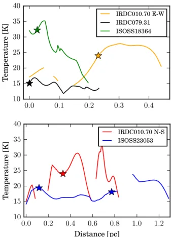
The first aspect is a challenging because we observe lower ammonia emission close to infrared emission sources (see Sect.4.2). Therefore it is difficult to measure the temperature at the position of infrared emission sources (e.g., ISOSS20153). To constrain the relation between infrared emission sources and the kinetic temperature, we extracted the temperature along several lines shown in Figs.1–3, and6and show the temperature distri-bution along these lines as a function of distance in Fig.10. We chose the 70 µm emission sources to be located along the line, and the location is marked in Fig.10. We find that some sources in our sample show increasing temperatures up to 30 K toward infrared emission sources (e.g., ISOSS23053 MM2, Fig. 10). These temperatures are even higher than the core temperatures reported in Ragan et al. (2012a). However, this could be due to the lower resolution of the Herschel observatory (∼11.400_for 160 µm).

The core temperatures determined in Ragan et al.(2012a) are average values over the entire core, but embedded protostars could heat the center of these cores significantly. Furthermore, the Herschel data probe dust temperatures, whereas the am-monia data probe gas temperatures. Our observations therefore agree with the picture that infrared emission sources imply an embedded protostar(s) that heats its environment. Wang et al. (2008) find similar results toward the northern region of the IRDC G28.34+0.06, which shows increasing temperatures to-ward the infrared emission source IRS 2 with a peak rotation temperature of 30 K. On the other hand,Ragan et al.(2011) re-port a quiescent temperature structure without correlating tem-perature peaks and infrared emission sources, which might be due to the early evolutionary stage of their sample.

This is also true for some of our sources, since they show no correlation between the temperature peaks and the infrared emission sources, e.g., IRDC079.31 (black line in Fig.10). For this source we see an ammonia temperature peak that is off-set to the infrared emission peak. Young embedded protostars, shown as infrared emission sources, are therefore not the only

0.0 0.1 0.2 0.3 0.4 10 15 20 25 30 35 40 Temperature [K] IRDC010.70 E-W IRDC079.31 ISOSS18364 0.0 0.2 0.4 0.6 0.8 1.0 1.2 Distance [pc] 10 15 20 25 30 35 40 Temperature [K] IRDC010.70 N-S ISOSS23053

Fig. 10.Temperature distribution as a function of the distance along the lines shown in the lower right panels of Figs.1–3, and6. In the top panel, the yellow, black, and green lines show the temperature distri-butions of the sources IRDC010.70 (along east-west), IRDC079.31 and ISOSS18364, respectively. The red and blue lines in the bottom panel show the temperature distributions of the sources IRDC010.70 (along north–south) and ISOSS23053, respectively. The x-axes (distance) are different for the top and bottom panels. The stars mark the positions of corresponding 70 µm emission sources.

heating source for dense gas traced by ammonia observations. Other mechanisms, such as turbulent motions, can heat the gas as well.

The second aspect, shielding of the clumps from the inter-stellar radiation field, would induce decreasing temperatures to-ward infrared dark regions. For smaller and less massive objects, Launhardt et al.(2013) report decreasing temperatures toward the center of starless cores from Herschel far-infrared dust obser-vations. They claim that this decrease is due to the shielding of the surrounding core and that only the outer envelope gets heated by the interstellar radiation field (e.g.,Zucconi et al. 2001). In the absence of strong infrared emission sources, this result can also be found for high-mass IRDCs.Wang et al.(2008) report a decreasing temperture of ∼15 K for the more quiescent southern region of G28.34+0.06.

In contrast to this, we do not identify any significant tem-perature decrease toward infrared dark regions within the two IRDCs of our sample (IRDC010.70, IRDC079.31). IRDC010.70 shows a prominent temperature peak within the northern infrared dark region of more than 35 K. IRDC079.31 shows a constant temperature distribution in the northern infrared dark region with a temperature peak on one side up to 17 K (see lower right panel of Fig.2). This temperature increase may be an indicator of on-going star formation at that position, which does not show any

far-infrared emission yet, or it indicates external heating from the interstellar radiation field.

5. Conclusions

We observed NH3 (1, 1) and (2, 2) lines of six IRDCs with the VLA and five out of these six with the Effelsberg 100 m Tele-scope. Our goal was to investigate the kinematics and temper-atures of these clumps and compare our results with Herschel infrared observations. Our main conclusions follow.

1. Our ammonia observations show a close spatial correla-tion with cold gas and dust, which is observed via infrared absorption or submillimeter continuum emission. We con-firmed that ammonia is a good tracer of dense gas. But we also found decreasing ammonia emission close to 24 µm emission sources, which has not been observed to date. 2. We found a temperature range from 10 to 30 K.

Tempera-tures higher than 30 K have to be treated cautiously, be-cause the method based on the low-excitation NH3 lines is not sensitive to higher temperatures. For some sources, we found a correlation between infrared emission sources and the temperature of the surrounding gas, which indicates that the embedded protostar heats up its environment. On the other hand, several infrared emission peaks do not coincide with ammonia temperature peaks. Because we observed a decreasing ammonia emission toward several infrared emis-sion sources, it is difficult to measure the temperature for these infrared emission peaks. Furthermore, we find temper-ature peaks in the ammonia data that do not coincide with any infrared emission. Other mechanisms, such as turbulent motions or external heating of the interstellar radiation field, can heat the gas.

3. We report an upper limit of ∼1.3 km s−1_{for the linewidth in} our sample. This is the spectral resolution limit of our ob-servation, and we do not see variations larger than this upper limit within our sources.

4. Half of our sources indicate evidence for gravitational col-lapse, either in the form of steep velocity steps or smooth velocity gradients, which are not consistent with rotation and therefore might represent gas flows.

5. The steep velocity gradient observed in ISOSS23053 is unique in our sample. We find two velocity components with a difference of 1.5 km s−1 _{and a gradient larger than} 30 km s−1 pc−1. Infrared and submillimeter observations show no evidence of different components. It is striking that different indicators of ongoing star formation are located close to the velocity step. As a result, the most likely ex-planation are signatures from a dynamical collapse and/or converging flows and sheer motions, which may initiate ac-tive star formation in this region. This interpretation agrees with recent theoretical models.

In summary, our data constrains the kinematic and thermody-namic initial conditions of star-forming regions in several ways. Although we did not identify collapse signatures in all fields, we do find evidence of gas flows and collapse motions in sev-eral clumps. The absence of these signatures in the remaining sources may indicate that they are either more evolved and the signatures have already vanished or that the NH3 observations are not an unambiguous tracer of gas flows and collapse motions. With respect to the temperature structure, we do see tempera-ture increases for some sources toward the more evolved parts of the clumps, indicated by infrared emission sources. On the other

hand, we find sources that show no clear correlation between in-frared emission sources and ammonia temperature peaks, which indicates that other mechanism, such as turbulent motions or the interstellar radiation field, can heat the gas as well.

Acknowledgements. Based on observations with the 100-m Telescope of the MPIfR (Max-Planck-Institut für Radioastronomie) at Effelsberg. The National Radio Astronomy Observatory is a facility of the National Science Foundation operated under cooperative agreement by Associated Universities, Inc. S.E.R. and R.J.S. acknowledge support from the DFG via the SPP 1573 Physics of the ISM (grants RA 2158/1-1 and SM321/1-1). R.J.S. also acknowledge support from the SFB 881 The Milky Way System.

References

Bergin, E. A., & Langer, W. D. 1997,ApJ, 486, 316

Bergin, E. A., & Tafalla, M. 2007,ARA&A, 45, 339

Beuther, H., & Henning, T. 2009,A&A, 503, 859

Beuther, H., & Sridharan, T. K. 2007,ApJ, 668, 348

Beuther, H., Churchwell, E. B., McKee, C. F., & Tan, J. C. 2007,Protostars and Planets V, 165

Beuther, H., Tackenberg, J., Linz, H., et al. 2012,A&A, 538, A11

Beuther, H., Linz, H., Tackenberg, J., et al. 2013,A&A, 553, A115

Birkmann, S. M., Krause, O., Hennemann, M., et al. 2007,A&A, 474, 883

Bogun, S., Lemke, D., Klaas, U., et al. 1996,A&A, 315, L71

Bonnell, I. A., Vine, S. G., & Bate, M. R. 2004,MNRAS, 349, 735

Brogan, C. L., Hunter, T. R., Cyganowski, C. J., et al. 2011,ApJ, 739, L16

Chira, R.-A., Beuther, H., Linz, H., et al. 2013,A&A, 552, A40

Csengeri, T., Bontemps, S., Schneider, N., Motte, F., & Dib, S. 2011a,A&A, 527, A135

Csengeri, T., Bontemps, S., Schneider, N., et al. 2011b,ApJ, 740, L5

Danby, G., Flower, D. R., Valiron, P., Schilke, P., & Walmsley, C. M. 1988,

MNRAS, 235, 229

de Wit, W. J., Testi, L., Palla, F., & Zinnecker, H. 2005,A&A, 437, 247

Devine, K. E., Chandler, C. J., Brogan, C., et al. 2011,ApJ, 733, 44

Di Francesco, J., Johnstone, D., Kirk, H., MacKenzie, T., & Ledwosinska, E. 2008,ApJS, 175, 277

Dunham, M. K., Rosolowsky, E., Evans, II, N. J., Cyganowski, C., & Urquhart, J. S. 2011,ApJ, 741, 110

Egan, M. P., Shipman, R. F., Price, S. D., et al.1998, ApJ, 494, L199

Evans, N. J., Shirley, Y. L., Mueller, K. E., & Knez, C. 2002, in Hot Star Workshop III: The Earliest Phases of Massive Star Birth, ed. P. Crowther,

ASP Conf. Ser., 267, 17

Goodman, A. A., Benson, P. J., Fuller, G. A., & Myers, P. C. 1993,ApJ, 406, 528

Gürtler, J., Klaas, U., Henning, T., et al. 2002,A&A, 390, 1075

Gvaramadze, V. V., Weidner, C., Kroupa, P., & Pflamm-Altenburg, J. 2012,

MNRAS, 424, 3037

Hennemann, M., Birkmann, S. M., Krause, O., & Lemke, D. 2008,A&A, 485, 753

Hennemann, M., Birkmann, S. M., Krause, O., et al.2009, ApJ, 693, 1379

Henning, T., Linz, H., Krause, O., et al. 2010,A&A, 518, L95

Hernandez, A. K., Tan, J. C., Kainulainen, J., et al. 2012,ApJ, 756, L13

Ho, P. T. P., & Townes, C. H. 1983,ARA&A, 21, 239

Kauffmann, J., Pillai, T., & Zhang, Q. 2013,ApJ, 765, L35

Klein, R., Posselt, B., Schreyer, K., Forbrich, J., & Henning, T. 2005,ApJS, 161, 361

Klessen, R. S. 2011, in EAS Pub. Ser. 51, eds. C. Charbonnel, & T. Montmerle, 133

Klessen, R. S., Ballesteros-Paredes, J., Vázquez-Semadeni, E., & Durán-Rojas, C. 2005,ApJ, 620, 786

Krause, O., Lemke, D., Vavrek, R., et al. 2003, in Galactic Star Formation Across the Stellar Mass Spectrum, eds. J. M. De Buizer, & N. S. van der Bliek,ASP Conf. Ser., 287, 174

Krause, O., Vavrek, R., Birkmann, S., et al. 2004,Baltic Astron., 13, 407

Lada, C. J., & Lada, E. A. 2003,ARA&A, 41, 57

Launhardt, R., Stutz, A. M., Schmiedeke, A., et al. 2013,A&A, 551, A98

Lu, X., Zhang, Q., Liu, H. B., Wang, J., & Gu, Q. 2014,ApJ, 790, 84

MacLaren, I., Richardson, K. M., & Wolfendale, A. W. 1988,ApJ, 333, 821

Millar, T. J., MacDonald, G. H., & Gibb, A. G. 1997,A&A, 325, 1163

Nomura, H., & Millar, T. J. 2004,A&A, 414, 409

Ossenkopf, V., & Henning, T. 1994,A&A, 291, 943

Perault, M., Omont, A., Simon, G., et al. 1996,A&A, 315, L165

Peretto, N., & Fuller, G. A. 2009,A&A, 505, 405

Pilbratt, G. L., Riedinger, J. R., Passvogel, T., et al. 2010,A&A, 518, L1

Pillai, T., Wyrowski, F., Menten, K. M., & Krügel, E. 2006b,A&A, 447, 929

Pineda, J. E., Goodman, A. A., Arce, H. G., et al. 2010,ApJ, 712, L116

Pitann, J., Hennemann, M., Birkmann, S., et al. 2011,ApJ, 743, 93

Purcell, C. R., Longmore, S. N., Walsh, A. J., et al. 2012,MNRAS, 426, 1972

Ragan, S. E., Bergin, E. A., & Gutermuth, R. A. 2009,ApJ, 698, 324

Ragan, S. E., Bergin, E. A., & Wilner, D. 2011,ApJ, 736, 163

Ragan, S., Henning, T., Krause, O., et al. 2012a,A&A, 547, A49

Ragan, S. E., Heitsch, F., Bergin, E. A., & Wilner, D. 2012b,ApJ, 746, 174

Rathborne, J. M., Simon, R., & Jackson, J. M. 2007,ApJ, 662, 1082

Rathborne, J. M., Jackson, J. M., Zhang, Q., & Simon, R. 2008,ApJ, 689, 1141

Rathborne, J. M., Jackson, J. M., Chambers, E. T., et al. 2010,ApJ, 715, 310

Redman, R. O., Feldman, P. A., Wyrowski, F., et al. 2003,ApJ, 586, 1127

Reid, M. J., Menten, K. M., Zheng, X. W., et al. 2009,ApJ, 700, 137

Sánchez-Monge, Á., Palau, A., Fontani, F., et al. 2013,MNRAS, 432, 3288

Schneider, N., Csengeri, T., Bontemps, S., et al. 2010,A&A, 520, A49

Simon, R., Rathborne, J. M., Shah, R. Y., Jackson, J. M., & Chambers, E. T. 2006,ApJ, 653, 1325

Smith, R. J., Shetty, R., Beuther, H., Klessen, R. S., & Bonnell, I. A. 2013,ApJ, 771, 24

Stahler, S. W., Palla, F., & Palla, F. 2005, The Formation of Stars (Physics Textbook), 1st edn. (Wiley-VCH)

Tafalla, M., Myers, P. C., Caselli, P., & Walmsley, C. M. 2004,A&A, 416, 191

Tan, J. C., Beltrán, M. T., Caselli, P., et al. 2014,Protostars and Planets VI, 149

Vasyunina, T., Linz, H., Henning, T., et al. 2009,A&A, 499, 149

Vasyunina, T., Vasyunin, A. I., Herbst, E., & Linz, H. 2012,ApJ, 751, 105

Wang, Y., Zhang, Q., Pillai, T., Wyrowski, F., & Wu, Y. 2008,ApJ, 672, L33

Wienen, M., Wyrowski, F., Schuller, F., et al. 2012,A&A, 544, A146

Williams, J. P., Blitz, L., & McKee, C. F. 2000,Protostars and Planets IV, 97

Wyrowski, F. 2008, in Massive Star Formation: Observations Confront Theory, eds. H. Beuther, H. Linz, & T. Henning,ASP Conf. Ser., 387, 3

Zhang, Q., & Wang, K. 2011,ApJ, 733, 26

Zhang, Q., Wang, Y., Pillai, T., & Rathborne, J. 2009,ApJ, 696, 268

Zijlstra, A. A., van Hoof, P. A. M., & Perley, R. A. 2008,ApJ, 681, 1296

Zinnecker, H., & Yorke, H. W. 2007,ARA&A, 45, 481

Zucconi, A., Walmsley, C. M., & Galli, D. 2001,A&A, 376, 650

Appendix A: Ammonia spectra

Table A.1. Summary of ammonia emission peaks shown in Figs.1–6.

Object α (J2000) δ (J2000) Tant(1, 1) Tant(2, 2) vpeak τpeak

Name [h:m:s] [◦

:0

:00

] [Jy beam−1_{] [Jy beam}−1_{] [km s}−1_]

IRDC010.70 p1 18:09:45.589 −19:42:08.800 0.056 0.038 28.8 3.4 IRDC079.31 100 m 20:31:57.800 40:18:19.900 1.49 0.43 1.59 3.0 IRDC079.31 p1 20:31:57.860 40:18:31.613 0.117 0.045 1.8 2.9 IRDC079.31 p2 20:31:57.545 40:18:21.213 0.106 0.034 1.6 3.6 ISOSS18364 100 m 18:36:36.000 −02:21:44.700 0.46 – 35.1 2.51 ISOSS18364 p1 18:36:35.735 −02:21:40.181 0.052 0.014 35.1 0.1 ISOSS20153 100 m 20:15:21.700 34:53:44.900 0.39 0.13 2.4 1.3 ISOSS20153 p1 20:15:21.928 34:53:28.807 0.086 0.016 2.1 0.4 ISOSS20153 p2 20:15:21.311 34:53:40.001 0.066 – 2.1 0.1 ISOSS22478 100 m 22:47:49.700 63:56:45.500 0.54 – −40.0 1.5 ISOSS22478 p1 22:47:50.027 63:56:47.414 0.068 – −40.4 0.3 ISOSS23053 100 m 23:05:21.900 59:53:50.000 1.53 0.62 −51.6 0.9 ISOSS23053 p1 23:05:23.563 59:53:58.409 0.070 0.022 −51.9 0.72 ISOSS23053 p2 23:05:21.755 59:53:44.016 0.110 0.031 −52.3 0.47

Notes. The position and fit parameter for the ammonia emission peaks as well as for the ammonia observations with the Effelsberg 100 m are given. The corresponding spectra are shown in Figs.A.1−A.6. As the VLA observations do not resolve the line width, we do not mention it here. The line widths of the Effelsberg 100 m observations are given in Table3.

10

15

20

25

30

35

40

45

v

[km s

]

−0.01

0.00

0.01

0.02

0.03

0.04

0.05

0.06

0.07

T

[Jy

beam

]

10

15

20

25

30

35

40

45

v

[km s

]

−0.01

0.00

0.01

0.02

0.03

0.04

VLA

NH

(1, 1)

NH

(2, 2)

Fig. A.1.VLA NH3spectra of IRDC010.70 at the position p1. Left-hand side: NH3(1, 1) spectra and right-hand side: NH3(2, 2) spectra. The red

line corresponds to the fit. As we do not observe the hyperfine structure of the NH3(2, 2) transition, we show a Gaussian fit to the main component.

−20

−10

0

10

20

v

[km s

]

−0.5

0.0

0.5

1.0

1.5

2.0

T

[Jy

beam

]

−20

−10

0

10

20

v

[km s

]

−0.2

−0.1

0.0

0.1

0.2

0.3

0.4

0.5

Effelsberg 100m

NH

(1, 1)

NH

(2, 2)

−20 −15 −10 −5

0

5

10

15

v

[km s

]

−0.02

0.00

0.02

0.04

0.06

0.08

0.10

0.12

T

[Jy

beam

]

−20 −15 −10 −5

0

5

10

15

v

[km s

]

−0.02

−0.01

0.00

0.01

0.02

0.03

0.04

0.05

0.06

VLA and Effelsberg

NH

(1, 1)

NH

(2, 2)

−20 −15 −10 −5

0

5

10

15

v

[km s

]

−0.02

0.00

0.02

0.04

0.06

0.08

0.10

0.12

T

[Jy

beam

]

−20 −15 −10 −5

0

5

10

15

v

[km s

]

−0.010

−0.005

0.000

0.005

0.010

0.015

0.020

0.025

0.030

0.035

VLA and Effelsberg

NH

(1, 1)

NH

(2, 2)

Fig. A.2. NH3 spectra of IRDC079.31. Left-hand side: NH3(1, 1) spectra and right-hand side: NH3(2, 2) spectra. Top two panels:

Effelsberg 100 m observations, central panels: combined VLA and Effelsberg 100 m spectra at the position p1 and bottom panels: combined VLA and Effelsberg 100 m spectra at the position p2. The red line corresponds to the fit. As we do not observe the hyperfine structure of the NH3(2, 2) transition, we show a Gaussian fit to the main component. The fit parameters and coordinates of the spectra are given in TableA.1.

20

30

40

50

v

[km s

]

−0.2

0.0

0.2

0.4

0.6

T

[Jy

beam

]

20

30

40

50

v

[km s

]

−0.3

−0.2

−0.1

0.0

0.1

0.2

0.3

Effelsberg 100m

NH

(1, 1)

NH

(2, 2)

15

20

25

30

35

40

45

50

v

[km s

]

−0.02

0.00

0.02

0.04

0.06

T

[Jy

beam

]

15

20

25

30

35

40

45

50

v

[km s

]

−0.015

−0.010

−0.005

0.000

0.005

0.010

0.015

VLA and Effelsberg 100m

NH

(1, 1)

NH

(2, 2)

Fig. A.3. NH3 spectra of ISOSS18364. Left-hand side: NH3(1, 1) spectra and right-hand side: NH3(2, 2) spectra. Top two panels:

Effelsberg 100 m observations and bottom panels: combined VLA and Effelsberg 100 m spectra at the position p1. The red line corresponds to the fit. As we do not observe the hyperfine structure of the NH3(2, 2) transition, we show a Gaussian fit to the main component. We do not detect

the NH3(2, 2) line for the Effelsberg 100 m observations within the uncertainties. The fit parameters and coordinates of the spectra are given in