HAL Id: hal-00304717
https://hal.archives-ouvertes.fr/hal-00304717
Submitted on 1 Jan 2002HAL is a multi-disciplinary open access archive for the deposit and dissemination of sci-entific research documents, whether they are pub-lished or not. The documents may come from teaching and research institutions in France or abroad, or from public or private research centers.
L’archive ouverte pluridisciplinaire HAL, est destinée au dépôt et à la diffusion de documents scientifiques de niveau recherche, publiés ou non, émanant des établissements d’enseignement et de recherche français ou étrangers, des laboratoires publics ou privés.
Feed-Forward Neural Network method used for river
flow forecasting
A. Y. Shamseldin, A. E. Nasr, K. M. O’Connor
To cite this version:
A. Y. Shamseldin, A. E. Nasr, K. M. O’Connor. Comparison of different forms of the Multi-layer Feed-Forward Neural Network method used for river flow forecasting. Hydrology and Earth System Sciences Discussions, European Geosciences Union, 2002, 6 (4), pp.671-684. �hal-00304717�
Comparison of different forms of the Multi-layer Feed-Forward
Neural Network method used for river flow forecasting
Asaad Y. Shamseldin
1, Ahmed E. Nasr
2and Kieran M. O’Connor
31Department of Civil Engineering, The University of Birmingham, Edgbaston, Birmingham B15 2TT, UK 2Department of Civil Engineering, University College Dublin, Earlsfort Terrace, Dublin 2, Ireland 3Department of Engineering Hydrology, National University of Ireland, Galway,Galway, Ireland
Email for corresponding author: [email protected]
Abstract
The Multi-Layer Feed-Forward Neural Network (MLFFNN) is applied in the context of river flow forecast combination, where a number of rainfall-runoff models are used simultaneously to produce an overall combined river flow forecast. The operation of the MLFFNN depends not only on its neuron configuration but also on the choice of neuron transfer function adopted, which is non-linear for the hidden and output layers. These models, each having a different structure to simulate the perceived mechanisms of the runoff process, utilise the information carrying capacity of the model calibration data in different ways. Hence, in a discharge forecast combination procedure, the discharge forecasts of each model provide a source of information different from that of the other models used in the combination. In the present work, the significance of the choice of the transfer function type in the overall performance of the MLFFNN, when used in the river flow forecast combination context, is investigated critically. Five neuron transfer functions are used in this investigation, namely, the logistic function, the bipolar function, the hyperbolic tangent function, the arctan function and the scaled arctan function. The results indicate that the logistic function yields the best model forecast combination performance.
Keywords: River flow forecast combination, multi-layer feed-forward neural network, neuron transfer functions, rainfall-runoff models
Introduction
River flow forecast combination is a methodology that simultaneously utilises the discharge forecasts of a number of different rainfall-runoff models to produce an aggregate discharge forecast which is generally superior to those of the individual models involved in the combination. The combinational methodology may be viewed as being a rather simple alternative to the iterative method of systematic model refinement for improving the accuracy of river flow forecasts (Shamseldin et al., 2000).
The combination concept is widely used in diverse fields, such as economics, business, statistics and meteorology (Clemen, 1989). However, in the context of river flow forecasting, the combination concept was introduced originally by McLeod et al. (1987) for combining the monthly river flows obtained from different time series models and it was further developed and investigated by Shamseldin (1996), Shamseldin et al. (1997) and Shamseldin and O’Connor (1999) using the daily discharge forecasts of different rainfall-runoff models. The theoretical
justification of the river flow forecast combination methodology is that each rainfall-runoff model provides an important source of information, which may differ from that of the other models. Thus, the ensemble of the information from such different sources would logically be expected to provide more accurate and reliable discharge forecasts.
A further justification for using the combination methodology in the context of river flow forecasting is that, at the present time, there is no ‘super-model’ available which performs better, under all circumstances, than the other available models. This fact is reflected in many of the inter-comparison studies of river flow forecasting models. The series of very useful but inconclusive model-intercomparison studies conducted by the World Meteorological Organisation (WMO, 1975, 1992) did not result in clear guidelines for model selection. Naef (1981) noted that neither simple nor complex rainfall-runoff models are free from failure in certain cases. Chiew et al. (1993) compared the performance of six rainfall-runoff modelling approaches of different levels of complexity. Their results
indicated that the complex conceptual models are capable of providing adequate estimates of daily flows in wet catchments whereas the simulation of daily flows for the drier catchments is generally poor. They also showed that the other modelling approaches considered, e.g. those of the black-box type and simple conceptual models, cannot provide consistently adequate flow estimates. Another notable model-intercomparison study is that of Perrin et al. (2001), who compared the performance of the structures of 19 lumped rainfall- runoff models using the daily data of 429 catchments located around the world. They found that the complex models generally out-performed the simpler models in the calibration period but not in the verification/ validation period. Many studies have also confirmed the equifinality characteristic of rainfall-runoff models, in the sense that structurally different models can produce quite similar results (cf. Loague and Freeze, 1985; Hughes, 1994; Franchini and Pacciani, 1991; Michaud and Sorooshian, 1994; Ye et al., 1997; Beven and Freer, 2001). This concept of equifinality is also applicable to sub-versions of an elaborate complex model, as it is often observed that simple sub-versions can produce similar results that are not substantially different from those of the elaborate form of the model (cf. Mein and Brown, 1978; Kachroo, 1992; Shamseldin, 1992; O’Connor, 1995; Lidén and Harlin, 2000). Indeed, the regular emergence of published reports on new models for river flow forecasting, such as those based on various neural network configurations, illustrates the clear perception among hydrologists that no single superior model has yet been developed.
The combined estimate of discharge, Qˆ , of a numberci
of N rainfall-runoff models, for the i-th time period is mathematically defined as (Shamseldin, 1996)
)
Qˆ
,
Qˆ
,...,
Qˆ
,....,
Qˆ
,
Qˆ
F(
=
c
Qˆ
i 1,i 2,i j,i N-1,i N,i (1)where F ( ) is the combination function and Qˆj,i is the estimated discharge of the j-th model. The river flow forecast combination methods are classified as being linear or non-linear methods, depending on the nature of the postulated combination function. The linear combination methods include the Simple Average Method (SAM) and the Weighted Average Method (WAM). In the naïve SAM, the combined forecast is simply the arithmetic average of the forecasts of the individual models. However, in the WAM, the combined forecast is the weighted sum of the forecasts of the individual rainfall-runoff models. The Neural Network Method (NNM), which uses neural network models for the production of the combined forecasts (Shamseldin et al., 1997), is an example of a non-linear combination method. The neural network may be visualised as a mathematical
technique for modelling systems without any a priori assumption regarding the explicit form of the relationship between the inputs and the outputs. In systems terminology, a neural network is normally regarded as a non-linear black-box model, which is calibrated using a set of input and output data.
In recent years, the neural network technique has become an increasingly popular modelling tool for river flow forecasting. This popularity can be gauged by the plethora of recent studies which have dealt with the application of neural networks in that context (Coulibaly et al., 2001; Kim and Barros, 2001; Chang and Chen, 2001; See and Abrahart 2001; Xiong et al., 2001; Tingsanchali and Gautam, 2000; Imrie et al., 2000; Gautam et al., 2000; See and Openshaw, 2000; Dawson and Wilby1998, 1999; Campolo et al., 1999; Sajikumar and Thandaveswara, 1999). A recent comprehensive review of the application of neural networks in hydrological and water resources modelling can be found in the works of Maier and Dandy (2000a) and Dawson and Wilby (2001). However, despite the claims made for their versatility and generality, it has not been demonstrated conclusively that these neural network river flow-forecasting models are in fact superior to the traditional models (See and Abrahart 2001; Lauzon et al., 2000; Tingsanchali and Gautam, 2000; Sajikumar and Thandaveswara, 1999; Shamseldin, 1997) and indeed the neural network models can prove to be quite disappointing. For example, the failure of these neural network models to capture the flood peaks has been reported in several flow simulation studies (Karunanithi, et al., 1994; See et al., 1997; Dawson and Wilby, 1998; Campolo et al., 1999).
Various forms of neural networks have been applied in various disciplines (Lippmann, 1987). However, in the context of hydrological modelling, the Multi-Layer Feed-Forward Neural Network (MLFFNN) is generally chosen because of its perceived versatility in function approximation (Shamseldin et al., 1997). The MLFFNN consists of a number of interconnected computational elements. These elements are known as neurons and they are arranged in a series of layers. The layers forming the MLFFNN are the input layer, the output layer and a number of intermediate layers between the input and the output layers. These intermediate layers are usually known as
hidden layers. Each neuron can be regarded as a multiple
input - single output sub-model. A mathematical function, known as the neuron transfer function, is used for transforming the neuron inputs into its single output.
In the case of the input layer, a linear transfer function is used. However, in the case of the hidden and output layers, a non-linear transfer function is used for both forms of layer. A consequence of the non-linearity of this transfer function
in the operation of the network, when so introduced, is that the network is thereby enabled to deal robustly with complex undefined relations between the inputs and the output. Thus, the selection of an appropriate transfer function is an important issue in the application of the MLFFNN. The most popular non-linear transfer function used in neural network studies is the logistic function (Blum, 1992, p. 39). However, there are various other types of non-linear transfer functions that can also be used in conjunction with the MLFFNN (cf. Fausett, 1994, pp. 17–19; Masters, 1993, pp. 81–82). According to the recent comprehensive review of neural network applications in water resources by Maier and Dandy (2000a), it appears that the logistic and the hyperbolic tangent functions are most widely used in such applications. In the context of salinity forecasting, Maier and Dandy (2000b) compared the performance of three MLFFNN models, which use three different neuron transfer functions, the linear threshold, the hyperbolic tangent and the sigmoid functions. However, in each case, the same transfer function was used for both the hidden and the output layers. The study showed that the results obtained using the linear threshold function were consistently the worst, whereas the results obtained using the hyperbolic tangent and the sigmoid functions were comparable, the results for the hyperbolic tangent function being only marginally better.
Imrie et al. (2000) investigated the effects on the overall performance of the MLFFNN river flow forecasting models of using four different transfer functions for the output neuron, the bipolar function being used for the hidden neurons. The results of the study indicated that the use of a cubic polynomial transfer function, or other transfer functions with a similar shape, in the output layer may be necessary for the neural networks to capture the extreme flood events successfully.
In Shamseldin (1996) and Shamseldin et al. (1997) on the MLFFNN river flow forecast combination method, only the logistic function was used in conjunction with the neurons in the hidden and the output layers. In the present study, the significance of using different non-linear transfer functions for the hidden and output layers is examined in the context of the overall performance of the MLFFNN river flow forecast combination method. Five neuron transfer functions are selected for this investigation, namely, the logistic function, the bipolar function, the hyperbolic tangent function, the arctan function and the scaled arctan function. To test which of these functions performs best, the discharge forecasts of five rainfall-runoff models, applied to eight catchments, are used. The five rainfall-runoff models are the Simple Linear (Total Response) Model (SLM) (Nash and Foley, 1982; Kachroo and Liang, 1992), the seasonally-based Linear Perturbation Model (LPM) (Nash and Barsi, 1983), the Linearly-Varying Variable Gain Factor Model (LVGFM) (Ahsan and O’Connor, 1994), the Constrained Linear System with a Single Threshold (CLS-Ts) (Todini and Wallis, 1977; Xia, 1989) and the Soil Moisture Accounting and Routing Procedure (SMAR) (O’Connell et
al., 1970; Kachroo, 1992; Khan, 1986; Liang, 1992). The
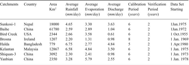
first four of these models are system-theoretical (black-box) models while the fifth is a lumped quasi-physical conceptual model. These models are described in considerable detail by Shamseldin et al. (1997). The eight test catchments are in different locations throughout the world (Table 1).
Table 1. Summary description of the eight test catchments.
Catchments Country Area Average Average Average Calibration Verification Data Set Km2 Rainfall Evaporation Discharge Period Period Starting
(mm/day) (mm/day) (mm/day) (years) (years)
Sunkosi-1 Nepal 18000 4.65 3.30 3.63 6 2 1Jan.1975
Baihe China 61780 2.59 2.89 1.04 6 2 1Jan.1972
Bird Creek USA 2344 2.66 3.58 0.61 6 2 1 Oct.1955
Brosna Ireland 1207 2.20 1.31 0.98 8 2 1 Jan. 1969
Halda Bangladesh 779 6.75 2.77 4.84 5 2 1 Apr.1980
Kelantan Malaysia 12867 6.58 4.84 3.50 6 2 1 Jan. 1975
Shiquan-3 China 3092 2.30 2.41 0.98 6 2 1 Jan. 1973
The Multi-Layer Feed-Forward
Neural Network (MLFFNN) method
used for river flow forecast
combination
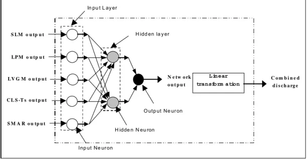
The Multi-Layer Feed-Forward Neural Network is one of the most widely used forms of neural network. The MLFFNN is capable of modelling the unknown input-output relations of a wide variety of complex systems. The structure of the MLFFNN used in the present study (Fig. 1) consists of only three layers; the input layer, the intermediate (hidden) layer and the output layer. Each layer contains a number of neurons (i.e. mathematical processing elements). Even though the neurons in any of the three layers are not linked to each other (e.g. the neurons of the hidden layer are not connected to each other), each neuron in the input layer is linked by connection pathways to all of the neurons in the following intermediate layer and likewise each neuron in the intermediate layer is linked by connection pathways to the single neuron in the output layer. Each neuron can receive a single input or an array of inputs, but it produces only a single output. In the case of the MLFFNN, the information flows successively only in the forward direction, i.e. from the input layer through the intermediate layer to the output layer. The connection pathways provide the means of transferring the information between any two consecutive layers.
The input layer receives all the external inputs to the network. In the context of river flow forecast combination, the external inputs to the network for a particular time period
are the discharge forecasts of the individual rainfall models for that time period. Each of the individual model forecasts is assigned to one neuron in the input layer. Thus, the number of neurons in the input layer is equal to the number of the rainfall-runoff models involved in the discharge-forecast combination procedure. For each of these neurons in the input layer, a direct linear transformation is used for the mapping of the neuron input to the neuron output according to
f(x) = x for all x. (2)
For each neuron of the input layer, its output then becomes the input to each of the neurons of the hidden layer.
The hidden layer is an intermediate layer between the input and the output layers. It is this layer that usually enhances the capability of the network to deal robustly and efficiently with inherently complex non-linear relations between the inputs and the output of the network (Medsker, 1994, p. 12). Of course, in contrast to the simple form of MLFFNN sketched in Fig. 1, the MLFFNN can have more than one hidden layer. However, the use of more than one hidden layer is rarely justified in practice (Masters, 1993, p. 174) and may well result in gross over-parameterisation of the model. Accordingly, a single hidden layer is used in the present study. Each hidden layer neuron has an input array but only a single output, connected to the single neuron of the output layer. Excluding the neurons of the input layer, the elements of the input array to a neuron are the final outputs of the corresponding neurons in the preceding layer,
S LM o u tp u t LP M o u tp u t LV G M o u t p u t S M A R o u tp u t CL S -T s o u t p u t N e tw o rk o u t p u t H idd en la y er In pu t L ay er O utp ut Ne ur on H idde n N eu ron Inp ut Ne ur on Linear transform ation C o m b i n e d d i s ch a rg e
Fig. 1. Schematic diagram for the Multi-layer Feed-Forward Neural Network used for combining the outputs of the
while its single output becomes an element for the input array of each of the neurons in the subsequent layer. Unlike the input layer, which has the same number of neurons as individual models providing their forecasts as inputs to that layer, the number of the neurons in the hidden layer is unknown a priori. There is no rule of thumb to specify the appropriate number of neurons in the hidden layer. In practical applications, this number can be estimated by an iterative process, which involves the calibration and the evaluation of the performance of the network using different assumed numbers of hidden layer neurons. The optimum number is that which has near-maximum efficiency using as few neurons as are necessary, i.e. the principle of parameter parsimony applies.
The output layer is the last layer in the network and it produces the final output of the network, i.e. the combined model discharge forecast. Similar to the neurons in the hidden layer, the output neuron receives an input array from the neurons of the preceding (hidden) layer and produces a single output, corresponding to the single neuron in the output layer. In the more general multiple-output case, there would be as many neurons in the output layer as network outputs. In the present study, only one neuron is required in that layer. In the case of hidden and output neurons, the process of transformation of the input array to a single output is quite similar. This transformation process is given by
) W W Y f( ) f(Y Y N i o 1 i i net out = =
∑
+ = (3) where Yout is the neuron output, f( ) is the selected neuron transfer function, N is the total number of the neurons in the preceding layer, Yi is the neuron input received from the neuron in the preceding layer, is the neuron net input, Wi is the connection weight assigned to the path linking the neuron to that i-th neuron and Wo is the neuron threshold value or bias. The neuron transfer function is non-linear and in the present study, similar to other studies, the same transfer function is used for all neurons in the hidden and the output layers. However, in the case of the output layer, linear functions can also be used. The most widely used non-linear transfer function in neural network applications is the logistic function (Blum, 1992, p. 39). The logistic function is bounded between 0 and +1 and is defined by ) Y Exp(-1 1 ) f(Y net net + = (4)However, a number of other non-linear transfer functions can be used in the case of hidden and output neurons of the
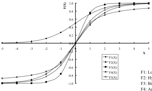
MLFFNN river flow-forecasting combination method. In the present study, in addition to the logistic function, the following four non-linear transfer functions are also considered in the application of the MLFFNN combination method;
1. The hyperbolic tangent function, which is bounded between –1 and +1, and expressed as
) Y 2 Exp( 1 ) Y 2 Exp( 1 ) Y Exp( ) Exp(Y ) Y Exp( ) Exp(Y ) f(Y net net net net net net net − + − − = − + − − = (5)
2. The bipolar function, which is a linear transformation of the logistic function, has output values varying between -1 and +1. This function is given by
) Y Exp( 1 ) Y Exp( 1 1 ) Y Exp( 1 2 ) f(Y net net net net − + − − = − − + = (6)
3. The arctan function, which has values ranging between –1 and +1, and is defined as
) arctan(Y π
2 )
f(Ynet = net (7)
4. The scaled arctan function, which is also bounded between –1 and +1. This function has the following form
(
sinh(Y ))
arctan π 2 )f(Ynet = net (8)
These four different neuron transfer functions are shown in graphical form in Fig. 2. From this figure, it can be seen that the hyperbolic tangent function and the scaled arctan function are quite similar in form.
The connection weights (Wi) and the neuron threshold values W0 constitute the parameters of the network. These parameters are estimated by an optimisation technique to minimise the sum of the squares of the errors. The use of the above bounded transfer functions for the output neuron implies that the estimated network output values are likewise bounded within the range of the selected transfer function. As the actual observed discharge values are usually outside this range, rescaling of the observed discharge values is required to facilitate comparison of the actual observed discharges and the network-estimated outputs. In the present study, the following linear rescaling function is used
) Q Q b( a Q max i si = + (9)
where Qsi is the rescaled discharge, a and b are the parameters of the rescaling function, Qi is the observed discharge and Qmax is the maximum actual observed discharge in the calibration period. In practical applications, the effective
o i N i i net YW W Y =
∑
+ =1range is usually less than that of the selected transfer function to avoid the occurrence of values near the extreme values because such values can affect the calibration of the network adversely. The use of such an effective range is also important to enable the network to predict discharge values greater than those occurring in the calibration period. In the case of the logistic function, the values of the rescaling parameters are chosen such that the Qsi series is bounded between 0.1 and 0.85. However, in the case of the other four non-linear transfer functions, which are bounded in the range [-1,1], the values of the rescaling parameters are chosen such that the Qsi series is between –0.85 and 0.85. Should linear transfer functions be used in the output layer, any rescaling of the observed outputs would become unnecessary.
Calibration of the Multi-Layer
Feed-Forward Neural Network
In the present study, the network parameters (i.e. connection weights (Wi) and the neuron threshold values W0) are estimated by minimising the least squares objective function (i.e. sum of the squares of the errors between the estimated and observed outputs) using a sequential search procedure. This sequential procedure involves the consecutive use of two optimisation methods:
(i) The genetic algorithm (GA) is a globally based search procedure introduced by Holland (1975). It is loosely
based on the Darwin theory of survival of the fittest where the potential solutions mate with each other in
order to produce stronger solutions (van Rooij et al.,
1996, pp. 18–24). The main characteristics of the GA are that it searches a population of solutions, uses probabilistic rules to advance the search and codes the parameter values as genes in a chromosome (cf. Khosla and Dillon, 1997, p. 46; Wang, 1991). The operation of the GA starts with an initial population of parameter sets which is randomly generated. Pairs of parameter sets are selected from this initial population according to their fitness evaluated on the basis of the selected objective function value. These pairs of parameter sets are then used to produce a new population of parameter sets (i.e. the next generation) according to the genetic operators of crossover and mutation. This new population is expected to be better than the old one. The process of generating new populations of parameter sets is repeated until the stopping condition is satisfied (i.e. the total number of function evaluations is reached). The GA was first applied in the context of calibrating conceptual catchment models by Wang (1991) (ii) The conjugate gradient method is a derivative-based
local search method suitable for optimisation in complex modelling problems. It is regarded as being more robust and efficient than the back-propagation method which is widely used for estimating the parameters of the MLFFNN (Masters, 1993, pp. 105–111). This method
-1.0 -0.8 -0.6 -0.4 -0.2 0.0 0.2 0.4 0.6 0.8 1.0 -5 -4 -3 -2 -1 0 1 2 3 4 5 X F(X) F1(X) F2(X) F3(X) F4(X) F5(X) F1: Logistic Function
F2: Hyperbolic Tangent Function F3: Bipolar Function
F4: Arctan Function F5: Scaled Arctan Function
adjusts the parameter values iteratively and requires determination of the objective function value, the corresponding gradient (i.e. the first order derivative) and a search direction vector to perform this iterative process (cf. Haykin, 1999, p. 243: Press et al., 1992, pp. 413–418). The search direction vector for any particular iteration is determined in such a way that it is conjugate to (i.e. linearly independent of) the previous search directions. The parameter values are adjusted by conducting line searches along the search direction vector. The method terminates when a stopping condition is satisfied (e.g. the maximum number of iterations, or the proscribed degree of convergence of the successive values of the objective function). In this sequential search procedure, the final optimised parameter values of the genetic algorithm are used as the initial starting values for the conjugate gradient method. The rationale behind the use of this sequential procedure is simply to maximise (or at least enhance) the likelihood of finding the global optimum parameter values.
Applications of the Multi-Layer
Feed-Forward Neural Network (MLFFNN)
as a river flow forecast combination
method
The MLFFNN river flow forecasting method, incorporating in turn the five different neuron transfer functions; the logistic, the bipolar, the hyperbolic tangent, the arctan and the scaled arctan, is tested using the discharge forecasts of five rainfall-runoff models, each operating on a total of eight test catchments. The five resulting models of the MLFFNN forecasting combination method are henceforth referred to as MLFFNN-1 (logistic function), MLFFNN-2 (bipolar function), MLFFNN-3 (hyperbolic tangent function), MLFFNN-4 (arctan function), and MLFFNN-5 (scaled arctan function), respectively. In each neural network model, the same transfer function is used for all the neurons in the hidden and the output layers. The available data for these catchments are split into two non-overlapping parts (i.e. split-sampling), the first part being used for calibration and the second part for verification. The lengths of the calibration and the verification periods for the eight catchments, as well as a brief summary description of these catchments, are shown in Table (1).
The number of neurons in the single hidden layer is taken as two and the MLFFNN is calibrated using the sequential optimisation procedure described earlier. In the present study, the number of hidden neurons is determined by a trial and error procedure in which the network is calibrated
(i.e. trained) successively with an increasing number of hidden neurons and the optimal number of neurons adopted for the hidden layer is generally that beyond which the performance of the network does not improve substantially with an increase of that number. In the present work, the optimal number selected is two simply because the corresponding results of the network are found to be either as good as or, in some cases, even better than those obtained using more than two neurons in the hidden layer.
The overall performance of the MLFFNN solutions and of the five individual rainfall-runoff models providing their inputs is assessed using the model efficiency criterion (E) of Nash and Sutcliffe (1970). This efficiency index E is given by 100 1 × o F F -E= (10)
where F is the sum of the squares of the differences between the estimated discharges and the corresponding observed discharges and Fo is the ‘initial variance’, which is defined as the sum of the squares of the differences between the observed discharges and the mean discharge of the calibration period.
Table 2 shows the E values of the five rainfall-runoff models for the eight test catchments. The SLM model is consistently the worst model among the five rainfall-runoff models considered, in both the calibration and the verification periods. The table also indicates that, in the calibration period, the SMAR model performs best for six out of the eight catchments; Bird Creek, Brosna, Halda, Kelantan, Shiquan-3 and Yanbian. For the remaining two catchments, Baihe and Sunkosi-1, the models having the best results are the LVGFM and the LPM, respectively. Likewise, in the verification period, the SMAR model has the highest E among the five models for five catchments, Bird Creek, Brosna, Halda, Kelantan and Yanbian. For the remaining three catchments, the LPM has the highest E values in the Sunkosi-1 and the Baihe catchments while the LVGFM has the highest E values in the Shiquan-3 catchment.
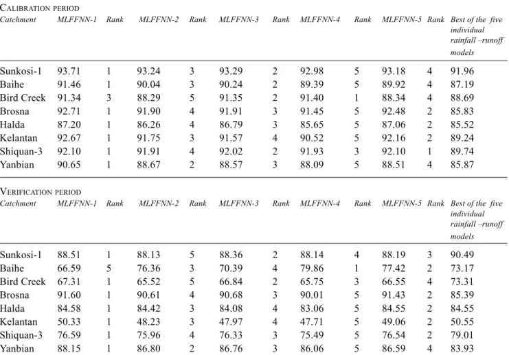
Table 3 displays the E values of the five different forms of the MLFFNN river flow forecasting method and their ranking for the eight test catchments. This table also displays the best E values among the five rainfall-runoff models. Inspection of Table 3 reveals that, in the calibration period, all five different forms of the MLFFNN combination method have higher E values than those obtained by the best of the five rainfall-runoff models. However, in the verification period, the results are quite variable. One or other form of the MLFFNN performs better than the best of the five
Table 2. E-efficiency values for the test catchments obtained using
the five individual rainfall-runoff models applied in the combination. CALIBRATIONPERIOD
Catchment (E) SLM (E) LPM (E) LVGFM (E) CLS-Ts (E) SMAR
Sunkosi-1 85.78 91.96 88.63 90.52 89.81 Baihe 70.46 74.30 87.19 83.31 83.32 Bird Creek 59.52 63.54 86.10 65.35 88.69 Brosna 40.12 70.28 41.37 46.95 85.83 Halda 81.70 84.58 83.62 83.99 85.52 Kelantan 62.81 76.71 78.91 79.49 89.24 Shiquan-3 72.01 76.85 87.63 75.76 89.74 Yanbian 73.66 83.00 78.05 81.59 85.87 VERIFICATIONPERIOD
Catchment (E) SLM (E) LPM (E) LVGFM (E) CLS-Ts (E) SMAR
Sunkosi-1 83.37 90.49 83.59 84.62 85.19 Baihe 70.52 73.17 61.45 65.50 72.79 Bird Creek -53.21 -38.99 24.90 -43.72 73.31 Brosna 45.68 77.53 48.06 60.25 85.39 Halda 72.38 77.18 75.31 66.53 84.55 Kelantan 37.49 37.89 43.84 37.49 50.55 Shiquan-3 54.02 56.16 79.01 57.30 68.16 Yanbian 75.74 79.21 76.38 81.10 83.93
rainfall-runoff models for four catchments, namely, Baihe, Brosna, Halda and Yanbian.
Table 3 also indicates that, for some of the test catchments, the differences in the E values among the five forms of the MLFFNN combination method are very marginal indeed. They also indicate that, in the calibration period, MLFFNN-1 (logistic function) has a better performance than other forms of MLFFNN for all of the test catchments, with the exception of Bird Creek, where it has only the third best performance. Furthermore, in the calibration period, MLFFNN-4 (arctan function) has the worst performance for six catchments, namely, Sunksoi-1, Baihe, Brosna, Halda, Kelantan, and Yanbian. However, MLFFNN-4 has the best performance only in the case of Bird Creek catchment for which its corresponding E value is not significantly different from those of MLFFNN-3 and MLFFNN-1.
Further comparison of the performance of the five MLFFNN models reveals that, in the calibration period, the performance of MLFFNN-2 ranks third in the case of three catchments, fourth for three catchments and for the remaining two catchments its performance rank is second and fifth. Likewise, the rank of the performance of
MLFFNN-3 is second in the case of four catchments, third for three catchments and fourth for one catchment. Similarly, the performance of MLFFNN-5 is best for one catchment, second best in the case of three catchments, and fourth for the other four catchments.
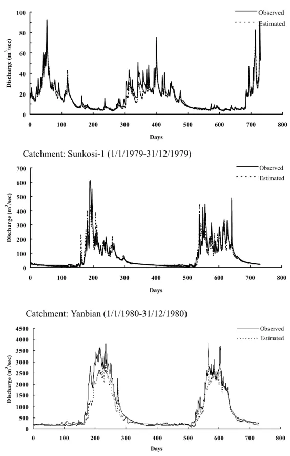
In the verification period, MLFFNN-1 has higher E value than the other four MLFFNN in all of the eight test catchments, with the exception of the Baihe catchment, for which its E value is the lowest among the five MLFFNNs. Likewise, the performance of the MLFFNN-2 form is ranked second in the case of one catchment, third for three catchments, fourth for two catchments and fifth for one catchment. The performance of MLFFNN-3 is ranked second for two catchments, third for three catchments, and fourth for three catchments also. MLFFNN-4 has the highest performance in the case of only one catchment while its performance is ranked third and fourth for two catchments, but for the remaining five catchments it has the worst performance. The performance of MLFFNN-5 is ranked second best for five catchments, while for the remaining three its rank is either third or fourth. Figure 3 shows compar-isons between the observed and the estimated discharge hydrographs of MLFFNN-1 for some selected catchments.
Table (3): E-efficiency values for the test catchments obtained using the five different Multi-Layer Feed-forward Neural Networks.
CALIBRATIONPERIOD
Catchment MLFFNN-1 Rank MLFFNN-2 Rank MLFFNN-3 Rank MLFFNN-4 Rank MLFFNN-5 Rank Best of the five
individual rainfall –runoff models Sunkosi-1 93.71 1 93.24 3 93.29 2 92.98 5 93.18 4 91.96 Baihe 91.46 1 90.04 3 90.24 2 89.39 5 89.92 4 87.19 Bird Creek 91.34 3 88.29 5 91.35 2 91.40 1 88.34 4 88.69 Brosna 92.71 1 91.90 4 91.91 3 91.45 5 92.48 2 85.83 Halda 87.20 1 86.26 4 86.79 3 85.65 5 87.06 2 85.52 Kelantan 92.67 1 91.75 3 91.57 4 90.52 5 92.16 2 89.24 Shiquan-3 92.10 1 91.91 4 92.02 2 91.93 3 92.10 1 89.74 Yanbian 90.65 1 88.67 2 88.57 3 88.09 5 88.51 4 85.87 VERIFICATIONPERIOD
Catchment MLFFNN-1 Rank MLFFNN-2 Rank MLFFNN-3 Rank MLFFNN-4 Rank MLFFNN-5 Rank Best of the five
individual rainfall –runoff models Sunkosi-1 88.51 1 88.13 5 88.36 2 88.14 4 88.19 3 90.49 Baihe 66.59 5 76.36 3 70.39 4 79.86 1 77.42 2 73.17 Bird Creek 67.31 1 65.52 5 66.84 2 65.75 3 66.55 4 73.31 Brosna 91.60 1 90.61 4 90.68 3 90.01 5 91.43 2 85.39 Halda 84.58 1 84.42 3 84.08 4 83.06 5 84.55 2 84.55 Kelantan 50.33 1 48.23 3 47.97 4 47.71 5 49.06 2 50.55 Shiquan-3 76.59 1 75.96 4 76.33 3 75.49 5 76.54 2 79.01 Yanbian 88.15 1 86.80 2 86.76 3 86.06 5 86.59 4 83.93
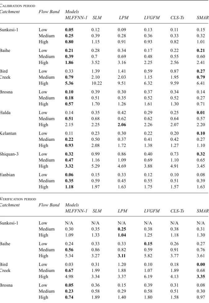
Table 4 shows the Normalised Root Mean Squared Error (NRMSE) of MLFFNN-1 (the best, on average, of the five MLFFNN models) and the five rainfall models for the different flow bands, low, medium and high. The discharge values exceeded 95% and 10% of the time in the calibration period are chosen subjectively as the upper limits of these two flow bands, respectively. The NRMSE is obtained by standardising the RMSE by the mean discharge of the calibration period, Q. The NRSME is calculated according to the following equation
Q m Q Q NRMSE m i i i
∑
= − = 1 2 ) ˆ ( (11)where Qˆi is the estimated discharge and m is the number of data points in the corresponding flow band. An NRMSE value of zero indicates a perfect model matching of the observed discharges in the flow band. In general, the higher
the value of the NRMSE the worse is the model performance. The NRMSE is used in this study to compare the performances of the different models in reproducing the discharge values in the different flow bands.
Examination of Table 4 shows that, in the calibration period, MLFFNN-1 has a better performance than the five individual rainfall-runoff models in the case of the medium and the high flow bands in all of the eight test catchments, except in the case of the Bird Creek and Halda catchments. In the Bird Creek catchment, the performance of MLFFNN-1 in the medium flow band is not significantly different from that of the best of the five rainfall-runoff models. In the Halda catchment, the performance of MLFFNN-1 in the high flow band is better than those of the lowest four models. However, in the case of the low flow band, MLFFNN-1 performs better than the five models in the case of three out of the eight catchments, Sunkosi-1 Brosna and Yanbian. For two out of the remaining five catchments, Baihe and Shiquan-3, the performance of MLFNN-1 in the low flow band is virtually the same as that of the best individual model.
Table 4. NRMSE values for the MLFFNN-1 form and the five individual rainfall-runoff models.
CALIBRATIONPERIOD
Catchment Flow Band Models
MLFFNN-1 SLM LPM LVGFM CLS-Ts SMAR Sunkosi-1 Low 0.05 0.12 0.09 0.13 0.11 0.15 Medium 0.25 0.39 0.28 0.36 0.33 0.32 High 0.80 1.15 0.91 0.93 0.82 1.01 Baihe Low 0.21 0.28 0.34 0.17 0.22 0.21 Medium 0.39 0.7 0.69 0.48 0.55 0.60 High 1.86 3.52 3.16 2.25 2.56 2.41 Bird Low 0.33 1.39 1.41 0.59 0.87 0.27 Creek Medium 0.79 2.10 2.03 1.15 1.95 0.79 High 5.36 10.22 9.51 6.32 9.59 6.41 Brosna Low 0.10 0.39 0.30 0.37 0.34 0.14 Medium 0.18 0.51 0.35 0.52 0.52 0.27 High 0.57 1.70 1.26 1.61 1.30 0.71 Halda Low 0.14 0.35 0.42 0.29 0.25 0.01 Medium 0.51 0.68 0.62 0.62 0.64 0.57 High 2.15 2.25 2.06 2.26 2.07 2.20 Kelantan Low 0.11 0.23 0.30 0.22 0.20 0.10 Medium 0.22 0.50 0.37 0.41 0.42 0.27 High 0.93 2.08 1.72 1.38 1.27 1.10 Shiquan-3 Low 0.32 0.99 0.86 0.40 0.73 0.32 Medium 0.47 1.16 1.09 0.69 1.10 0.65 High 3.32 5.29 4.69 3.88 4.91 3.45 Yanbian Low 0.06 0.15 0.33 0.12 0.10 0.08 Medium 0.35 0.59 0.45 0.55 0.51 0.39 High 1.18 1.97 1.63 1.75 1.57 1.63 VERIFICATIONPERIOD
Catchment Flow Band Models
MLFFNN-1 SLM LPM LVGFM CLS-Ts SMAR
Sunkosi-1 Low N/A N/A N/A N/A N/A N/A
Medium 0.30 0.35 0.25 0.38 0.38 0.31 High 1.09 1.33 1.04 1.25 1.18 1.30 Baihe Low 0.24 0.33 0.33 0.15 0.26 0.27 Medium 0.56 0.86 0.82 0.59 0.91 0.76 High 5.34 3.27 3.11 5.82 3.77 3.61 Bird Low 0.03 0.31 1.20 0.10 0.18 0.00 Creek Medium 0.67 1.99 1.88 1.07 1.89 0.68 High 4.98 3.34 3.37 6.19 4.13 3.35 Brosna Low 0.05 0.36 0.15 0.39 0.31 0.08 Medium 0.23 0.58 0.29 0.58 0.51 0.30 High 0.74 1.89 1.40 1.80 1.58 0.97
Halda Low 0.07 0.10 0.33 0.07 0.08 0.01 Medium 0.45 0.65 0.58 0.60 0.69 0.48 High 1.82 1.28 1.20 1.70 2.07 1.22 Kelantan Low 0.28 0.26 0.35 0.25 0.21 0.23 Medium 0.41 0.51 0.55 0.41 0.44 0.35 High 3.64 3.92 3.51 4.06 4.30 3.93 Shiquan-3 Low 0.30 0.90 0.79 0.31 0.44 0.32 Medium 0.81 1.59 1.53 1.02 1.60 1.17 High 6.44 7.51 7.52 5.47 7.38 7.02 Yanbian Low 0.07 0.29 0.26 0.17 0.14 0.07 Medium 0.37 0.57 0.46 0.61 0.53 0.39 High 1.58 1.99 2.17 1.70 1.62 2.01
For the other three catchments, Bird Creek, Halada and Kelantan, the performance of MLFFNN-1 is worse than that of the best of the five models, but still better than those of the lowest four individual models.
In the verification period, MLFFNN-1 results are quite variable. In the high flow band, MLFFNN-1 is at least better than the second best model for five catchments, namely, Sunkosi-1, Brosna, Kelantan, Shiquan-3 and Yanbian. In the remaining three catchments, it is only better than that of the worst individual model. In the medium flow band, MLFFNN-1 performs better than the individual models for six catchments. In the remaining two catchments, Sunkosi-1 and Kelantan, its performance is either not significantly different from or better than the second best model. In the low flow band, MLFFNN-1 performs consistently better than the second best model for all of the test catchments, except the Kelantan catchment where its performance is only better than worst individual model.
Possible links between the performance of MLFFNN-1 and the meteorological and hydrological characteristics of the catchments were also investigated in this study. Table 5 shows the correlation between the model efficiency index (E) of MLFFNN-1 and the coefficient of variation (CV) of the rainfall, evaporation and discharge in the calibration
period. The table also shows the correlation between E and the catchment area. For comparison, the corresponding correlation coefficients of the SMAR model (the best, on average, of the five individual models) are also included in the table. The table shows that in MLFFNN-1, high E values are associated with low rainfall CV values and high evaporation CV values. In the case of the SMAR model, high E values are associated with high discharge CV values and small catchment areas. The correlation coefficients shown in Table (5) are calculated on the basis of a small sample (8 catchments) and thus may be affected by sampling variability. Numerous catchments need to be used to calculate these coefficients to confirm the adequacy of the correlation patterns revealed in Table 5.
Conclusions
The effect on the overall performance of the Multi-Layer Feed-Forward Neural Network (MLFFNN) of using different transfer function types in the hidden and the output neurons, when applied in the context of the river flow forecast combination method, is examined. Five neuron transfer functions are considered in this investigation, namely, the logistic, bipolar, hyperbolic tangent, arctan and
Table 5. Correlation of the coefficient of Efficiency (E) of the MLFFNN-1 form and the SMAR model with
meteorological and hydrological characteristics of the catchment for the calibration period.
Correlation Coefficient
Model Rainfall CV Evaporation CV Discharge CV Catchment Area
E (MLFFNN-1) -0.58 0.42 -0.19 0.18
0 20 40 60 80 100 0 100 200 300 400 500 600 700 800 Days Discharge (m 3 /sec) Observed Estimated
Catchment: Sunkosi-1 (1/1/1979-31/12/1979)
0 100 200 300 400 500 600 700 0 100 200 300 400 500 600 700 800 Days Discharge (m 3 /sec) Observed Estimated 0 500 1000 1500 2000 2500 3000 3500 4000 4500 0 100 200 300 400 500 600 700 800 Days Discharge (m 3 /sec) Observed EstimatedFig. 3. Comparison of the observed and the simulated discharge hydrographs of the MLFFNN-1 form in the
verification period for some of the test catchments.
Catchment: Brosna (1/4/1973-1/4/1974)
References
Ahsan, M. and O’Connor, K.M., 1994. A simple non-linear rainfall-runoff model with a variable gain factor. J. Hydrol.,
155, 151–183.
Beven, K. and Freer, J., 2001. Equifinality, data assimilation, and uncertainty estimation in mechanistic modelling of complex environmental systems using the GLUE methodology. J.
Hydrol., 249, 11–-29.
Blum, A., 1992. Neural networks in C++; an object-oriented
framework for building connectionist systems. Wiley Inc., USA.
Campolo, M., Soldati, A. and Andreussi, P., 1999. Forecasting river flow rate during low-pow periods using neural networks.
Water Resour. Res., 35, 3547–3552.
Chang, F.J. and Chen, Y.C., 2001. A counterpropagation fuzzy-neural network modeling approach to real time streamflow prediction J. Hydrol., 245, 153–164.
Chiew, F.H.S., Stewardson, M.J. and McMahon, T.A., 1993. Comparison of six rainfall-runoff modelling approaches. J.
Hydrol. , 147, 1–36
Clemen, R.T., 1989. Combining forecasts: A review and annotated bibliography. Int. J. Forecasting, 5, 559–583.
Coulibaly P., Bobee, B. and Anctil, F., 2001. Improving extreme hydrologic events forecasting using a new criterion for artificial neural network selection. Hydrol. Process, 15, 1533-1536. Dawson, C.W. and Wilby, R., 1998. An artificial neural network
approach to rainfall-runoff modelling. Hydrolog. Sci. J., 43, 47–66.
Dawson, C.W. and Wilby, R.L., 1999. A comparison of artificial neural networks used for river flow forecasting. Hydrol Earth
Syst. Sc., 3, 529–540.
Dawson, C.W. and Wilby, R.L., 2001. Hydrological Modelling using artificial neural networks. Prog. Phys. Geog., 25, 80– 108.
Fausett, L., 1994. Fundamentals of neural networks: architectures,
algorithms, and applications. Prentice-Hall International., Inc.,
USA.
Franchini, M. and Pacciani, M., 1991. Comparative analysis of several conceptual rainfall-runoff models. J. Hydrol., 122, 161– 219.
Gautam, M.R., Watanabe, K. and Saegusa, H., 2000. Runoff analysis in humid forest catchment with artificial neural network.
J. Hydrol., 235, 117–136.
Haykin, S., 1999. Neural Networks a comprehensive foundation. Prentice Hall, USA.
Holland, J.H., 1975. Adaptation in natural and artificial systems. University Michigan Press, Ann Arbor.
Hughes, D.A., 1994. Soil Moisture and runoff simulation using four catchment rainfall-runoff models. J. Hydrol., 158, 381– 404.
Imrie, C.E., Durucan, S. and Korre, A., 2000. River flow prediction using artificial neural networks: generalisation beyond the calibration range. J. Hydrol., 233, 138–153.
Kachroo, R.K., 1992. River Flow forecasting. Part 5. Applications of a conceptual model. J. Hydrol., 133, 141–178.
Kachroo, R.K. and Liang, G.C., 1992. River flow forecasting. Part 2. Algebraic development of linear modelling techniques.
J. Hydrol., 133, 17–40.
Karunanithi, N., Grenney, W.J., Whitley, D. and Bovee, K., 1994. Neural networks for river flow prediction. J. Comput. Civil Eng.,
8, 201–220.
Khan, H., 1986. Conceptual Modelling of rainfall-runoff systems. M.Eng. Thesis, National University of Ireland.
Khosla, R. and Dillon, T., 1997. Engineering intelligent hybrid multi-agent systems. Kluwer, Dordrecht, The Netherlands. Kim, G. and Barros, A.P., 2001. Quantitative flood forecasting
using multisensor data and neural networks. J. Hydrol., 246, 45–62.
Lauzon, N., Rousselle, J., Birikundavyi, S. and Trung, H.T., 2000. Real-time daily flow forecasting using black-box models, diffusion processes, and neural networks. Can. J. Civil Eng.,
27, 671–682.
Liang, G.C., 1992. A note on the revised SMAR model. Dept. of Eng. Hydrology, University College Galway, Ireland (Unpublished).
Lidén, R. and Harlin J., 2000. Analysis of conceptual rainfall-runoff modelling performance in different climates. J. Hydrol.,
238, 231–247.
Lippmann, R. P., 1987. An introduction to computing with neural nets. IEEE ASSP Magazine, 4–22.
Loague, K.M. and Freeze, R.A., 1985. A comparison of rainfall-runoff modelling techniques on small upland catchments. Water
Resour. Res., 21, 229–249.
Maier, H.R. and Dandy, G.C., 2000a. Neural networks for the prediction and forecasting of water resources variables: a review of modelling issues and applications. Environ. Model. Softw.,
15, 101–124.
Maier, H.R. and Dandy, G.C., 2000b. The effects of internal parameters and geometry on the performance of back-propagation neural networks: an empirical study. Environ.
Model. Softw., 13, 193–209.
Masters, T., 1993. Practical neural networks recipes in C++. Academic Press, Inc., USA.
McLeod, A.I., Noakes, D.J., Hipel, K.W. and Thompstone, R.M., 1987. Combining hydrologic forecasts. Water Resour. Plann.
Mang., 113, 29–41.
Medsker, L.R., 1994. Hybrid Neural Network and Expert systems. Kluwer Academic Publishers, USA.
scaled arctan functions. The daily discharge forecasts of five rainfall-runoff models, applied to the data of eight catchments, are used in this investigation as the inputs to the various forms of neural network.
Overall, the results of the study indicate that when the
logistic function is used as the neuron transfer function, the
MLFFNN forecast combination procedure generally has the best results, whereas when the arctan function is used the MLFFNN generally has the worst results. However, the results also reveal that the differences in the model efficiency (E) values, when different neuron transfer functions are used, are quite marginal in some cases. This would suggest that, in these cases, the performance of the MLFFNN is rather insensitive to the type of transfer function used.
The results of the present study, based on the Multi-Layer Feed-Forward Neural Network (MLFFNN), lend further support to the previous findings of Shamseldin (1996) and Shamseldin et al. (1997), which showed that judiciously combined discharge forecasts can be significantly more reliable and accurate than those of the best of the individual rainfall-runoff models involved in the forecast combination method.
Mein, R.G. and Brown, B.M., 1978. Sensitivity of optimized parameters in watershed models. Water Resour. Res., 14, 229– 303.
Michaud, J. and Sorooshian, S., 1994. Comparison of simple versus complex distributed models on mid-sized semiarid watersheds. Water Resour. Res., 30, 539–605.
Naef, F., 1981. Can we model the rainfall-runoff process today?.
Hydrol. Sci. Bull., 26, 281–289.
Nash, J.E. and Barsi, B.I., 1983. A hybrid model for flow forecasting on large catchments. J. Hydrol., 65, 125–137. Nash, J.E. and Foley, J.J., 1982. Linear models of rainfall-runoff
systems. In: Rainfall-Runoff Relationship, V.P. Singh (Ed.), Proceedings of the International Symposium on Rainfall-Runoff modelling. Mississippi State University, May 1981, USA, Water Resources Publications. 51–66.
Nash, J.E. and Sutcliffe, J.V., 1970. River flow forecasting through conceptual models. Part 1. A discussion of principles. J. Hydrol.,
10, 282–290.
O’Connell, P.E., Nash J.E. and Farrell, J.P., 1970. River Flow forecasting through conceptual models. Part 2. The Brosna catchment at Ferbane. J. Hydrol., 10, 317–-329.
O’Connor, K.M., 1995. River flow forecasting: The Galway
experience. Invited Lecture, Symposium on River Flow
Forecasting and Disaster Relief, Haikou City, China, Nov. 20-25, 1995.
Perrin, C., Michel, C. and Andréassian, V., 2001. Does a large number of parameters enhance model performance? Comparative assessment of common catchment model structures on 429 catchments. J. Hydrol., 242, 275–301.
Press, W.H., Flannaery, B.P., Teukolsky, S.A. and Vetterling, W.T., 1992. Numerical Recipes. Cambridge University press, New York.
Sajikumar, N. and Thandaveswara, B.S., 1999. A non-linear rainfall-runoff model using an artificial neural network. J.
Hydrol., 216, 32–55.
See, L. and Abrahart, R.J., 2001. Multi-model data fusion for hydrological forecasting. Comput. Geosci., 27, 987–994. See, L. and Openshaw, S., 2000. A hybrid multi-model approach
to river level forecasting. Hydrolog. Sci. J., 45, 523–536. See, L., Corne, S., Doughetry, M. and Openshaw, S., 1997. Some
intial experiments with neural network models for flood forecasting on the River Ouse. Proceedings of the 2nd
International Confrence on GeoComputation. Dunedin, New Zealand.
Shamseldin, A.Y., 1992. Studies on conceptual rainfall-runoff
modelling. M.Sc. thesis, National University of Ireland, Galway.
(Unpublished).
Shamseldin, A.Y., 1996. Fundamental Studies in Rainfall-Runoff
Modelling. Ph.D thesis, National University of Ireland, Galway.
(Unpublished).
Shamseldin, A.Y., 1997. Application of Neural Network Technique to Rainfall-Runoff Modelling. J. Hydrol., 199, 272_294. Shamseldin, A.Y. and O’Connor, K.M., 1999. A real-time
combination Method for the outputs of different rainfall-runoff models. Hydrol. Sci. J., 44, 895–912.
Shamseldin, A.Y., O’Connor, K.M. and Liang, G.C., 1997. Methods for combining the outputs of different rainfall-runoff rodels. J. Hydrol., 197, 203–229.
Shamseldin, A.Y., Ahmed, E.N. and O’Connor, K.M., 2000. A
Seasonally Varying Weighted Average Method for the Combination of River Flow Forecasts. The XXth Conference of
the Danube Countries on Hydrological Forecasting and Hydrological Bases of Water Management, Bratislava, The Slovak Republic, September 2000.
Tingsanchali, T. and Gautam, M.R., 2000. Application of tank, NAM, ARMA and neural network models to flood forecasting.
Hydrol. Process, 14, 2473–2487.
Todini, E. and Wallis, J.R., 1977. Using CLS for daily or longer period rainfall-runoff modelling. In: Mathematical Models for
Surface Water Hydrology, T.A. Ciriani, U. Maione and J.R.
Wallis (Eds.), Proceedings of the Workshop of IBM Scientific Centre, Pisa, Italy. Wiley, New York. 149–168.
van Rooij, A.J.F., Jain, L.C. and Johnson, R.P., 1996. Neural
Network training using genetic algorithms. World Scientific
Publishing, USA.
Wang, Q.J., 1991. The genetic algorithm and its application to calibrating conceptual rainfall-runoff models. Water Resour.
Res., 27, 2467–2471.
World Meteorological Organization (WMO), 1975.
Intercomparison of conceptual models used in operational hydrological forecasting. Oper Hydrol. Rep. 7, WMO No. 429,
Geneva.
World Meteorological Organization (WMO), 1992. Simulated
real-time intercomparison of hydrological models. Oper Hydrol. Rep.
38, WMO No. 779, Geneva.
Xia, J., 1989. Part 2: Non-linear system approach. Research report of the 3rd International Workshop on River Flow Forecasting. University College Galway, Ireland (unpublished).
Xiong, L.H., Shamseldin, A.Y. and O’Connor, K.M., 2001. A non-linear combination of the forecasts of rainfall-runoff models by the first-order Takagi-Sugeno fuzzy system. J. Hydrol., 245, 196–217.
Ye, W., Bates, B.C., Viney, R., Sivapalan, M. and Jakeman, A.J., 1997. Performance of conceptual rainfall-runoff models in low-yielding ephemeral catchments. Water Resour. Res., 33, 153– 166.