HAL Id: hal-00302332
https://hal.archives-ouvertes.fr/hal-00302332
Submitted on 1 Dec 2006HAL is a multi-disciplinary open access
archive for the deposit and dissemination of sci-entific research documents, whether they are pub-lished or not. The documents may come from teaching and research institutions in France or abroad, or from public or private research centers.
L’archive ouverte pluridisciplinaire HAL, est destinée au dépôt et à la diffusion de documents scientifiques de niveau recherche, publiés ou non, émanant des établissements d’enseignement et de recherche français ou étrangers, des laboratoires publics ou privés.
The global impact of supersaturation in a coupled
chemistry-climate model
A. Gettelman, D. E. Kinnison
To cite this version:
A. Gettelman, D. E. Kinnison. The global impact of supersaturation in a coupled chemistry-climate model. Atmospheric Chemistry and Physics Discussions, European Geosciences Union, 2006, 6 (6), pp.12433-12468. �hal-00302332�
ACPD
6, 12433–12468, 2006 Impact of supersaturation A. Gettelman and D. E. Kinnison Title Page Abstract Introduction Conclusions References Tables Figures ◭ ◮ ◭ ◮ Back CloseFull Screen / Esc
Printer-friendly Version Interactive Discussion
EGU
Atmos. Chem. Phys. Discuss., 6, 12433–12468, 2006 www.atmos-chem-phys-discuss.net/6/12433/2006/ © Author(s) 2006. This work is licensed
under a Creative Commons License.
Atmospheric Chemistry and Physics Discussions
The global impact of supersaturation in a
coupled chemistry-climate model
A. Gettelman and D. E. Kinnison
National Center for Atmospheric Research, Boulder, CO, USA
Received: 3 November 2006 – Accepted: 22 November 2006 – Published: 1 December 2006 Correspondence to: A. Gettelman ([email protected])
ACPD
6, 12433–12468, 2006 Impact of supersaturation A. Gettelman and D. E. Kinnison Title Page Abstract Introduction Conclusions References Tables Figures ◭ ◮ ◭ ◮ Back CloseFull Screen / Esc
Printer-friendly Version Interactive Discussion
EGU Abstract
Ice supersaturation is important for understanding condensation in the upper tropo-sphere. Most general circulation models however do not permit supersaturation. In this study, a coupled chemistry climate model, the Whole Atmosphere Community Cli-mate Model (WACCM), is modified to include supersaturation for the ice phase. The 5
study is intended as a sensitivity experiment, to understand the potential impact of su-persaturation, and of expected changes to stratospheric water vapor, on climate and chemistry. Results indicate that high clouds decrease and water vapor in the strato-sphere increases nearly linearly with supersaturation (20% supersaturation increases water vapor by nearly 20%). The stratospheric Brewer-Dobson circulation slows at 10
high southern latitudes, consistent with slight changes in temperature likely induced by changes to cloud radiative forcing. The cloud changes also cause an increase in the seasonal cycle of near tropopause temperatures, increasing them in boreal summer over boreal winter. There are also impacts on chemistry, with small increases in ozone in the tropical lower stratosphere driven by enhanced production. The radiative impact 15
of changing water vapor is dominated by the reduction in cloud forcing associated with fewer clouds (∼+0.6 Wm−2) with a small component likely from radiative effect (green-house trapping) of the extra water vapor (∼+0.2 Wm−2), consistent with previous work. Representing supersaturation is thus important, and changes to supersaturation re-sulting from changes in aerosol loading for example, might have a modest impact on 20
global radiative forcing, mostly through changes to clouds. We do not see evidence of a strong impact of water vapor on tropical tropopause temperatures.
1 Introduction
Condensation in the atmosphere occurs when the vapor pressure of water or ice is higher than the saturation vapor pressure over liquid or ice (Murphy and Koop,2005). 25
ACPD
6, 12433–12468, 2006 Impact of supersaturation A. Gettelman and D. E. Kinnison Title Page Abstract Introduction Conclusions References Tables Figures ◭ ◮ ◭ ◮ Back CloseFull Screen / Esc
Printer-friendly Version Interactive Discussion
EGU
a fraction of a percent rarely persist, it is not true for ice processes (K ¨archer and Haag,
2004). Significant supersaturations over ice are seen routinely in the atmosphere from aircraft (Jensen et al., 2005), balloons and radiosondes (Spichtinger et al., 2003a) and satellites (Jensen et al.,1999;Spichtinger et al.,2003b;Gettelman et al.,2006). This is not surprising when one considers the condensation and freezing process for 5
molecules of H2O in the atmosphere. Freezing is essentially a 2 step process, requir-ing condensation and then freezrequir-ing (Koop et al., 2000). Since the saturation vapor pressure over water is higher than that over ice at low temperatures, we might then see large ice supersaturations before freezing occurs.
Supersaturation may have significant impacts on the state of the atmosphere. Mak-10
ing the most simple assumptions, if one allows 20% more water to be present before condensation, and stratospheric water vapor is limited by temperature dependent con-densation at the tropical tropopause (Holton and Gettelman, 2001), we might expect a corresponding increase of 20% in upper tropospheric and stratospheric water vapor, and a drop in high cloud cover. Changes to the condensation threshold would be due 15
to differences in water activity (Koop et al.,2000) which might arise due to variations in the population of aerosols for example.
Such changes would have significant impacts on climate and chemistry. Changes in high cloud cover would have significant effects on tropospheric climate and the radia-tion balance of the atmosphere. A reducradia-tion in high clouds may substantially increase 20
outgoing longwave radiation at the top of the atmosphere, leading to a cooling effect on the climate system. Alternatively, since the overall effect of clouds is to cool (Cess,
2005) a reduction in clouds might warm the planet.
Changes in stratospheric water may have effects on both chemistry and climate. Since water is the dominant species in the stratospheric hydrogen budget, we might 25
also expect differences in hydrogen radicals (HOx = OH + HO2) in the stratosphere, leading to changes in ozone and other trace species chemistry, particularly where hydrogen radicals dominate ozone chemistry in the lower stratosphere (Wennberg
ACPD
6, 12433–12468, 2006 Impact of supersaturation A. Gettelman and D. E. Kinnison Title Page Abstract Introduction Conclusions References Tables Figures ◭ ◮ ◭ ◮ Back CloseFull Screen / Esc
Printer-friendly Version Interactive Discussion
EGU
impact tropospheric temperatures (Forster and Shine, 2002). Recently Stuber et al.
(2001) and others (Stuber et al., 2005; Joshi et al., 2003) have speculated about a “stratospheric water vapor feedback” whereby changes in greenhouse gases force in-creases in tropopause temperatures, and these temperature changes induce inin-creases in stratospheric water which may further increase tropospheric temperatures.
5
Most global models, however, use large-scale closure schemes for condensation that include assumptions that do not permit supersaturation with respect to liquid or ice (for example,Rasch and Kristjansson,1998). For very large (100s of km) regions represented by global model grid cells this was thought to be a reasonable assumption. However, recent work with aircraft data (Gierens and Spichtinger,2000) on long flight 10
tracks and with satellites (Gettelman et al.,2006) has shown that even at these scales supersaturation may be present.
To better understand potential aerosol indirect effects on climate, more detailed treat-ments of ice cloud nucleation and microphysics are being developed for global models. Including representations of supersaturation will be critical for appropriately nucleating 15
ice clouds (K ¨archer et al.,2006) and for representing the affects of aerosol nucleation and freezing for ice clouds (K ¨archer and Lohmann,2002a,b).
Thus representation of supersaturation in global models is critically important for un-derstanding both stratospheric chemistry and tropospheric climate. In this work we present simple modifications to a coupled chemistry climate model which permit bulk 20
supersaturation with respect to ice, and use the model to understand the impact of su-persaturation on simulated climate and chemistry of the upper troposphere and lower stratosphere (UT/LS) region. This is not necessarily the ideal treatment of supersatura-tion, but within the context of a coupled chemistry climate model it allows us to examine the impact of supersaturation and increased stratospheric water vapor in a geophysical 25
way and understand feedbacks on stratospheric chemistry and atmospheric dynamics. The model and methodology is described in Sect. 2, the results are presented in Sect. refsec:results and conclusions are contained in Sect.4.
ACPD
6, 12433–12468, 2006 Impact of supersaturation A. Gettelman and D. E. Kinnison Title Page Abstract Introduction Conclusions References Tables Figures ◭ ◮ ◭ ◮ Back CloseFull Screen / Esc
Printer-friendly Version Interactive Discussion
EGU
2 Methodology
The principle behind this work is to take a state of the art coupled chemistry climate model, and allow grid box averaged supersaturation in the simulations. Below we de-scribe the model, the simple changes we have made, and the simulations we have performed. The purpose is not so much to evaluate the performance of the simulations 5
against observations but to examine the differences as a result of supersaturation. 2.1 Model description
For this work we have utilized the Whole Atmosphere Community Climate Model, Version 3 (WACCM3) developed at the National Center for Atmospheric Research (NCAR). WACCM3 is a state of the art coupled chemistry climate model that spans 10
the atmosphere from the surface to the lower thermosphere (∼140 km). The model is described by Garcia et al. (2006)1, and performs well relative to observations and to other coupled models (Eyring et al., 2006). We note some of the relevant features for this study below.
WACCM3 is based on the framework of the Community Atmosphere Model, ver-15
sion 3 (CAM3), a General Circulation Model (GCM), described byCollins et al.(2006). WACCM3 uses CAM3 as its base, and adds parameterizations for chemistry and up-per atmospheric processes. The CAM model top is typically 2 hPa (45 km), while the WACCM model top is 5×10⁻⁶hPa (140 km). The chemistry module for WACCM3 is derived from the three dimensional chemical transport Model for Ozone and Related 20
chemical Tracers (MOZART) (Brasseur et al.,1998;Horowitz et al.,2003; Kinnison et al., 20062). The chemistry package comprises 56-species representing chemical and
1
Garcia, R. R., Marsh, D., Kinnison, D., Boville, B. A., and Sassi, F.: Simulations of secular trends in the middle atmosphere, 1950–2003, J. Geophys. Res., submitted, 2006.
2
Kinnison, D. E., Brasseur, G. P., Walters, S., et al.: Sensitivity of Chemical Tracers to Meteorological Parameters in the MOZART-3 Chemical Transport Model, J. Geophys. Res., submitted, 2006.
ACPD
6, 12433–12468, 2006 Impact of supersaturation A. Gettelman and D. E. Kinnison Title Page Abstract Introduction Conclusions References Tables Figures ◭ ◮ ◭ ◮ Back CloseFull Screen / Esc
Printer-friendly Version Interactive Discussion
EGU
physical processes in the middle atmosphere, including inorganic nitrogen, hydrogen, chlorine and bromine chemistry, along with CH4 and its degradation products. Hetero-geneous processes on sulfate aerosols and polar stratospheric clouds are included. Surface fluxes of chemical species as well as NOx (NO+NO2) and CO sources from lightning and aircraft emissions are included, as are wet and dry deposition. The chem-5
istry is coupled in-line to the model dynamics and radiation, so that chemical species (such as ozone) affect model heating rates.
WACCM3 uses CAM3 routines for condensation and the hydrologic cycle. The model has a bulk microphysics scheme with prognostic vapor, liquid and ice that are con-served and advected (Rasch and Kristjansson, 1998). Fractional cloudiness is the 10
trigger for condensation and it is constrained by relative humidity (RH) followingSlingo
(1987), such that condensation begins at 90% relative humidity. CAM uses a “com-bined” relative humidity that reflects relative humidity with respect to water for temper-atures above –10◦C, with respect to ice below –30◦C, and a linear combination of the saturation vapor pressure between these limits. The simulation of the hydrologic cycle 15
is described byBoville et al.(2006). 2.2 Supersaturation
Because the bulk microphysics formulation of Rasch and Kristjansson (1998) used in WACCM3 does not permit supersaturation with respect to ice, we have modified the formulation of the Slingo (1987) cloud fraction scheme so that the critical relative 20
humidity threshold for starting to form cloud increases when ice is present, and can be higher than 100% RH. In the standard WACCM3 case, cloud begins to form at a relative humidity of 90%, and 100% cloud cover occurs at 100% RH. This has been modified for ice clouds so that cloud does not begin to form until RH=100% and full (100%) cloud cover occurs at RH=120%. These values are the model “merged” relative humidity. As 25
noted above, this means that for temperatures below –30◦C, condensation will not fully occur until RH=120% over ice.
ACPD
6, 12433–12468, 2006 Impact of supersaturation A. Gettelman and D. E. Kinnison Title Page Abstract Introduction Conclusions References Tables Figures ◭ ◮ ◭ ◮ Back CloseFull Screen / Esc
Printer-friendly Version Interactive Discussion
EGU
model. Other approaches, such as the treatment of K ¨archer and Lohmann(2002a), allow proper representation of condensation of ice through homogeneous and/or het-erogeneous nucleation and freezing of cloud particles on to aerosols. However, the bulk representation described above is internally consistent with the WACCM3 hydro-logic cycle, and we hypothesize that this will increase the amount of water vapor and 5
decrease condensation and clouds in the simulation in a geophysically realistic way. Other model simulations which have attempted to investigate the effect of increases in stratospheric water vapor have generally fixed water or explicitly enhanced its con-centration (e.g.Forster and Shine,2002, Stuber et al.,2005 and Stenke and Grewe,
2005).
10
2.3 Simulations
For analysis, two 22 year integrations of WACCM3 were performed at 4◦×5◦horizontal resolution. The model has 66 levels in the vertical with resolution of about 1km in the UT/LS region. In one (Base) simulation the standard WACCM3 configuration was used with annually repeating 1995 boundary conditions. This includes Sea Surface Tem-15
peratures from 1995 and levels of CO2 and chlorine compounds appropriate for that year. An identical “supersaturated” (SSAT) simulation was run with the same bound-ary conditions, but with the code modified to allow supersaturation for the ice phase as described above. The last 15 years of model output is used for all analyzes. We have repeated the analyzes in this paper on varying sets of 5 and 10 year periods from 20
each one. All the conclusions are qualitatively robust relative to inter-annual variations. There are some quantitative differences in the extra-tropics where variability is larger, but the conclusions are unchanged.
ACPD
6, 12433–12468, 2006 Impact of supersaturation A. Gettelman and D. E. Kinnison Title Page Abstract Introduction Conclusions References Tables Figures ◭ ◮ ◭ ◮ Back CloseFull Screen / Esc
Printer-friendly Version Interactive Discussion
EGU
3 Results
In this section we discuss the main results from comparing the two WACCM3 simula-tions, referred to as the “Base” and “SSAT” (or “supersaturated’) cases. We will first discuss cloud and water vapor fields since these are most directly impacted by the changes. We will then discuss the impact on the circulation (transport) and temper-5
ature, including chemical tracers of transport. We will then discuss ozone and other chemical species, and finally examine the radiative balance of the simulations and how they are related to other differences.
3.1 Clouds
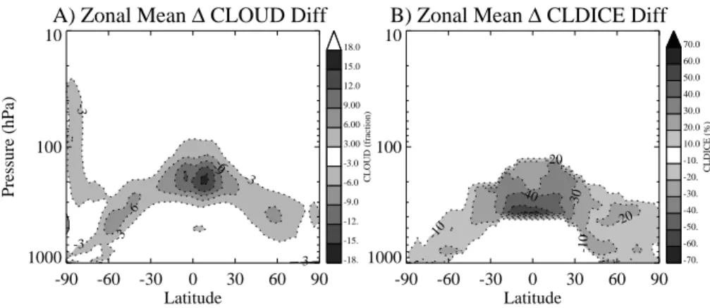
In the tropics, the maximum zonal mean cloud fraction for high clouds in the base simu-10
lation is found at 200–250 hPa (0.4). At the tropopause, cloud fraction is 0.2. The latter is almost exclusively cirrus clouds generated from the stratiform cloud parameteriza-tion. By raising the threshold for high (ice) cloud formation, the mean cloud fraction is decreased by nearly 50% (absolute, cloud fraction goes down by 0.17), as indicated in Fig.1a. At pressures above 600 hPa the differences are minor. The largest decreases 15
are at 200 hPa and coincident with the maximum high level cloudiness. There are smaller changes at high latitudes. Analysis of cloud changes sorted by optical depth indicates that most of the changes are to high clouds with optical depth less than 3 (cirrus clouds). Regionally the largest changes occur where the cloud fractions are highest, in the tropical Western Pacific region. Changes are larger in June–August 20
than in December–February.
Consistent with the change in cloudiness, cloud ice mixing ratio goes down almost everywhere in the simulations with supersaturation (Fig. 1b). In the tropical upper troposphere, the change is up to –50% and maximizes near the freezing level. Cloud liquid is less affected. As a result total precipitable water decreases by only 10% in 25
tropics (not shown).
ACPD
6, 12433–12468, 2006 Impact of supersaturation A. Gettelman and D. E. Kinnison Title Page Abstract Introduction Conclusions References Tables Figures ◭ ◮ ◭ ◮ Back CloseFull Screen / Esc
Printer-friendly Version Interactive Discussion
EGU
global mean precipitation. The global increase in both rate and total is about 4%, and occurs mostly in the central to eastern Pacific Inter-Tropical Convergence Zone (ITCZ), and over the Atlantic ocean. There are slight decreases in precipitation over the Indian Ocean. It is likely that the delay of condensation is causing precipitation to occur at a higher rate, though it is not clear why this would affect total precipitation, except if the 5
changes were to actually change the lifetime of humidity in the troposphere. The base simulation generally has too much precipitation in the central to eastern Pacific and the Indian ocean.
The radiative impact of clouds is usually assessed by examining the cloud forcing, which is the difference of the top of atmosphere radiation and the radiation assuming 10
a clear sky (e.g.Ramanathan et al.,1989). Short and longwave cloud forcing are cal-culated from the model using this method. With supersaturation and a reduction in cloudiness, the magnitudes of both shortwave and longwave forcing drop. The global average longwave cloud forcing is 30 Wm−2 in the base case, and drops by 7 Wm−2. The shortwave cloud forcing is –53 Wm−2(clouds cool in the shortwave), and drops by 15
–8 Wm−2(to –45 Wm−2) The net cloud forcing in the model is –22 Wm−2and changes by +0.6 Wm−2. We expect reductions in longwave forcing with the reduction in cirrus clouds, but the magnitude of the reductions is large enough to strongly reduce short-wave cloud forcing as well (and slightly more than the total longshort-wave forcing), particu-larly over the Indian Ocean. The cloud forcing changes appear largely due to changes 20
in simulated cirrus clouds. Changes in clouds are slightly larger during June–August than during December–February.
3.2 Water vapor
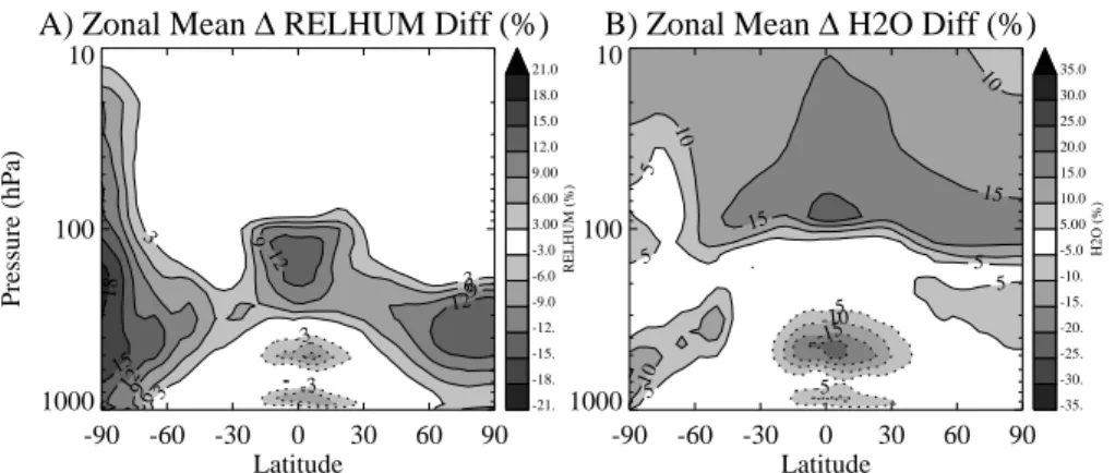
Like the changes in cloudiness, the changes in water vapor are expected from the changes to the physics in the simulation. In general, with the reduction in condensation, 25
specific humidity and relative humidity (RH) increase in the upper troposphere through-out the stratosphere. This is illustrated in Fig.2. Where RH is highest in the tropical UT/LS region and at high polar latitudes, RH increases by up to 12–15% (Fig. 2a).
ACPD
6, 12433–12468, 2006 Impact of supersaturation A. Gettelman and D. E. Kinnison Title Page Abstract Introduction Conclusions References Tables Figures ◭ ◮ ◭ ◮ Back CloseFull Screen / Esc
Printer-friendly Version Interactive Discussion
EGU
There are slight decreases in humidity at lower altitudes, below 300 hPa in the tropical middle troposphere, which is very close to the average freezing level in the simulations. This is perhaps due to raising of the condensation level. Water vapor (specific humid-ity) increases as well in the regions where the large scale cloudiness scheme controls its value: mostly in the tropical tropopause layer (Fig.2b). Note that RH increases in 5
the stratosphere as well, but the values are insignificant. Water vapor increases of up to 20% are seen just above the tropical tropopause, with values increasing everywhere in the stratosphere, but by lower percentage amounts as air is further from the tropical tropopause and RH is only a few percent.
Understanding the seasonality of these changes is critical for understanding their 10
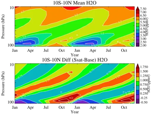
cause. Water vapor values in the tropical lower stratosphere have a strong seasonal cycle (Mote et al.,1996) with a minimum in boreal winter and a maximum in boreal sum-mer. This signal propagates vertically from the tropical tropopause as the air ascends due to the Brewer-Dobson circulation (Holton et al., 1995). The simulated “tropical tape recorder” signal (Mote et al.,1996) in water vapor from the base run is illustrated 15
in the top panel of Fig.3. Figure3shows a composite repeated annual cycle based on monthly means of the base simulation.
In general the annual cycle in the base WACCM3 simulation (top panel of Fig. 3) compares quite well to observations of water vapor in the stratosphere (Randel et al.,
2001;SPARC,2000). The minimum in water vapor occurs 1–2 months later than
ob-20
servations in the simulation, but the speed of propagation and attenuation is appropri-ate. Mixing ratios in the base case are generally 0.5 ppmv dry relative to observations, slightly more dry in boreal summer. For a full discussion of WACCM3 performance in this regard, see Garcia et al. (2006)1.
The lower panel of Fig.3 illustrates the differences between the model with super-25
saturation and the base case. Consistent with Fig. 2, water vapor increases almost everywhere, except in the troposphere below 100 hPa from January–March.
The increases are largest in boreal summer and fall from September–November. This is the period when cooling of the tropical tropopause region is strongly affecting
ACPD
6, 12433–12468, 2006 Impact of supersaturation A. Gettelman and D. E. Kinnison Title Page Abstract Introduction Conclusions References Tables Figures ◭ ◮ ◭ ◮ Back CloseFull Screen / Esc
Printer-friendly Version Interactive Discussion
EGU
water vapor. Note that the differences between the simulations occur in the lower stratosphere and also propagate vertically. Overall there is nearly 1 part per million by volume (ppmv) more water vapor in the stratosphere in the supersaturation case. Overall the changes improve the simulation of water vapor in the stratosphere. In order to determine the cause of these changes, it is instructive to examine changes in 5
temperature as well. 3.3 Temperature
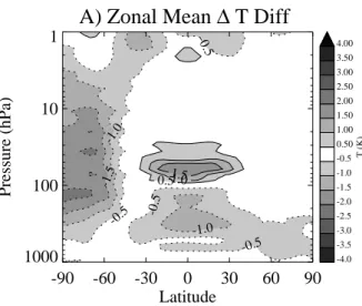
Figure4illustrates the annual zonal mean change in temperature between the simula-tions. There are slight and coherent changes in temperature in the simulations with su-persaturation. In general there are decreases of annual mean temperature in the upper 10
tropical troposphere by 0.5–1◦K. These changes may be due to several factors. First, the increase in water vapor in the upper troposphere will increase clear sky cooling. Second, the decrease in cloud fraction decreases any heating due to local absorption by clouds and increases the effect of the clear sky cooling. The region of cooling in the tropical upper troposphere (400–100 hPa) in Fig.4is similar to the region of reduced 15
cloudiness in Fig.1a. In the lower stratosphere there is an increase in temperature of up to 1.5◦K. This is consistent with decreased clouds below this region leading to more longwave absorption in the lower stratosphere. It may also indicate changes in the strength of the stratospheric wave-driven Brewer-Dobson circulation, which will be discussed in more detail below. Consistent with a change in the global circulation, 20
there are colder temperatures in the southern polar stratosphere. At 85 hPa, the spa-tial pattern of tropical temperature changes has increases nearly everywhere along the equator, with maximum changes over the equatorial eastern Pacific, and the equatorial western Pacific. In the upper stratosphere and mesosphere, there is cooling of up to 1.5 K (not shown), consistent with increased water vapor throughout the stratosphere 25
below.
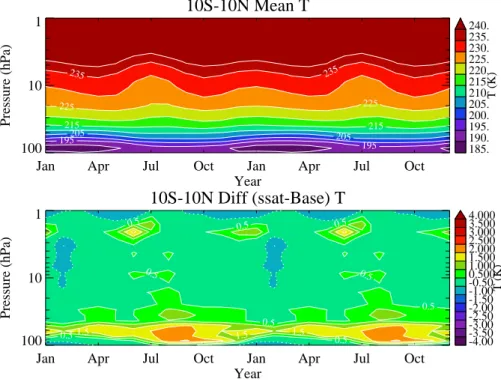
The temperature changes are not symmetric throughout the year. Figure5is similar to Fig.3but illustrates the equatorial temperature distribution up to 1hPa. Temperatures
ACPD
6, 12433–12468, 2006 Impact of supersaturation A. Gettelman and D. E. Kinnison Title Page Abstract Introduction Conclusions References Tables Figures ◭ ◮ ◭ ◮ Back CloseFull Screen / Esc
Printer-friendly Version Interactive Discussion
EGU
decrease slightly where water vapor in Fig.3decreases, and the largest temperature increases near the tropopause in Fig.5b are coincident with the largest water vapor increases at this level (Fig.3b). Thus it appears that temperature changes are affect-ing the annual cycle in water vapor differences between the simulations. There are still increases in stratospheric water vapor everywhere in the supersaturation simulation. 5
Consistent with Fig. 5b, tropical cold point tropopause temperature in the supersatu-ration simulation warms by 1◦K in boreal summer, with virtually no change in boreal winter. High latitude changes in temperature in the southern polar stratosphere are also largest in September–November (not shown).
Thus, the amplitude of the annual cycle of temperature around the tropical 10
tropopause increases in the supersaturation case, with larger temperature changes in July–October than in December–March. This appears to be due to larger changes (reductions) in tropical high clouds in boreal summer, with the result that there is an extra 5–15 Wm−2 of outgoing longwave radiation in this season, which is the likely cause of the warm temperatures. Seasonal changes to the residual circulation in the 15
stratosphere may also play a role.
3.4 Circulation and long lived trace species
Given the decreases in temperature seen at high latitudes in Fig.4and the increases in temperature in the tropics, it is obvious to ask if circulation changes might account for this difference. A decrease in the equatorial upwelling and corresponding decrease in 20
high latitude descent would alter temperatures in a similar manner to Fig.4, increasing temperatures in the tropics (reduced adiabatic cooling) and decreasing them at high latitudes (decreased adiabatic warming). To better understand the stratospheric circu-lation, we have calculated the Transformed Eulerian Mean (TEM) circulation (Andrews
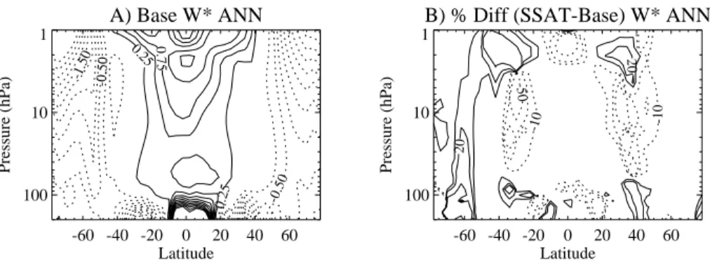
et al.,1987) for both runs. The annual residual mean vertical motion ( ¯w*) for the base
25
case is plotted in Fig. 6a, and features upward motion in the tropics and downward motion at the poles.
ACPD
6, 12433–12468, 2006 Impact of supersaturation A. Gettelman and D. E. Kinnison Title Page Abstract Introduction Conclusions References Tables Figures ◭ ◮ ◭ ◮ Back CloseFull Screen / Esc
Printer-friendly Version Interactive Discussion
EGU
simulations. Relative to the base case, down-welling at high latitudes of the southern hemisphere in the supersaturation run is 20% lower. In addition, there is a reduction of the meridional gradient of the circulation in the middle stratosphere: increases on the edges of the down-welling regions mean less (negative) down-welling, and decreases on the edges of the upwelling indicate less (positive) upwelling. These changes are 5
small however in absolute terms. There are slightly larger changes at higher altitudes (lower pressures) near 1 hPa. This is near the region where temperatures are cooling (Fig.4).
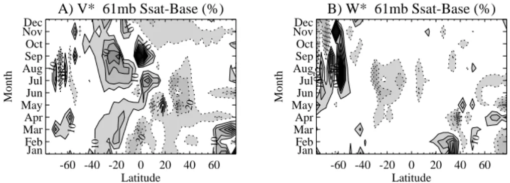
Figure 7 illustrates the annual cycle of the TEM meridional velocity, ¯v *, in Fig. 7a,
and the annual cycle of the TEM vertical velocity, ¯w*, in Fig. 7b, at 61 hPa, near the
10
maximum difference in tropical temperatures. In the tropics from May to September there are slight decreases in tropical upwelling (Fig.7b), which are consistent with the temperature changes in Fig.4. In addition, there are decreases in downward vertical velocity at high southern latitudes in Fig.7b. These changes are also consistent with changes to the vertical velocity. The horizontal velocity (Fig.7a), shows a decrease 15
in southward meridional flow in the supersaturation case throughout most of the year, and especially from July–October. These differences are associated with an increase in the speed of the southern hemisphere polar jet in the simulations.
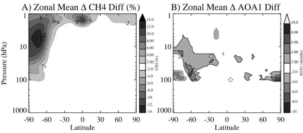
Another way of checking for consistency of the vertical motion changes is to examine long lived tracers. Figure8plots the percent change in concentration (mixing ratio) of 20
CH4 (Fig. 8a) and the temporal change in the Age of Air (Fig. 8b). Methane has a tropospheric source and decay in the stratosphere. Figure8a indicates decreases at southern polar latitudes, consistent with a slowing of the stratospheric circulation and (more time for chemical destruction). It does not appear as if there are changes in HOx to cause chemical changes in methane (see discussion of chemistry below).
25
A similar picture is also seen by calculating the Age of Air (Waugh and Hall,2002) in the stratosphere from the simulations (Fig.8b). Southern polar latitudes have an older age in the supersaturation simulation by 2–6 months (with a mean age of 4–4.5 years). This is consistent with the circulation and chemistry changes, indicating a slowing of
ACPD
6, 12433–12468, 2006 Impact of supersaturation A. Gettelman and D. E. Kinnison Title Page Abstract Introduction Conclusions References Tables Figures ◭ ◮ ◭ ◮ Back CloseFull Screen / Esc
Printer-friendly Version Interactive Discussion
EGU
the stratospheric circulation, with a change occurring mostly in Southern Hemisphere winter.
The simulations have also been examined for significant changes to the tropospheric circulation. In general there appear to be small changes in the northern hemisphere tropospheric circulation. The increase in the southern hemisphere stratospheric polar 5
jet appears to extend all the way to the surface (but changes are only of the order of 1–3 ms−1). There is virtually no change in the 200 hPa streamfunction.
3.5 Ozone and other species
The changes in temperature (Fig.4) and water vapor (Fig.2) due to allowing supersat-uration will also likely have impacts on chemistry in the UT/LS region and throughout 10
the stratosphere. One of the benefits of using WACCM3 is that changes to chemical species as a result of the changes to physics can be assessed in a consistent, coupled framework. One of the difficulties of using a coupled chemistry-climate model is that discerning causes in the coupled system is difficult (as will be shown below).
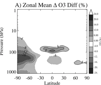
Figure 9plots the annual zonal mean percent difference in ozone between the two 15
simulations. O3increases in the tropical lower stratosphere by 5–10% in the supersatu-ration simulation. It decreases slightly in the middle troposphere, as well as decreasing by up to 18% in the southern hemisphere lowermost stratosphere.
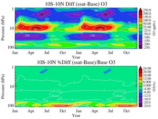
The seasonal cycle of tropical ozone changes is illustrated in Fig.10. The changes (in ppbv) in Fig.10a need to be taken in the context of ozone concentrations, so that 20
the middle stratospheric changes of ±200 ppbv are in percentage terms (Fig. 10b) smaller than the 50 ppbv change in the lower stratosphere. In the lower stratosphere, the ozone increase maximizes in July to October, and is consistent with the seasonal cycle of temperature (Fig.5) and water vapor (Fig.3) changes. This change in ozone is also consistent with slowing of the stratospheric circulation, which would allow more 25
time for ozone production in the tropical lower stratosphere. In the middle and upper stratosphere there is a “dipole” of decreases and then increases (Fig.10a) which are generally less than ±4% of the ozone concentration in Fig.10b). Note that the “dipole”
ACPD
6, 12433–12468, 2006 Impact of supersaturation A. Gettelman and D. E. Kinnison Title Page Abstract Introduction Conclusions References Tables Figures ◭ ◮ ◭ ◮ Back CloseFull Screen / Esc
Printer-friendly Version Interactive Discussion
EGU
is also consistent with decreased ozone in the middle stratosphere leading to increased UV penetration and increased ozone at lower levels (a “self-healing” effect). There are several other changes to the chemical balance of the UT/LS region, which occur in the supersaturation simulation and will help with interpreting the changes to ozone. These are discussed briefly below.
5
Increases in HOxare expected due to the changes in water vapor in the region. HOx increases in the supersaturation simulation by 15–20% in the lower tropical strato-sphere, located in the same region as the ozone (Fig. 9), temperature (Fig. 4) and water vapor (Fig.2) increases. Total reactive nitrogen (NOy) and the more active odd nitrogen molecules (NOx = NO + NO2) also change in the supersaturation case. The
10
increased HOx converts more NOx to HNO3, decreasing the NOx/NOy ratio between 5–10% (depending on altitude). This has the impact of reducing the odd-oxygen loss importance of NOy. The opposite is true for the total reactive chlorine (Cly) family. Here, increases in HOx convert more HCl to ClO, and increasing the ClO/HCl ratio by 5–20% (depending on altitude), increasing the odd-oxygen loss importance of the Cly
15
family. This chemical sensitivity of increased HOx repartitioning reservoir species to active forms in the NOy and Cly families is consistent with the discussion inDvortsov
and Solomon (2001).
In line with previous work (Stenke and Grewe,2005), we see a very small impact of increased H2O on ozone chemistry in the stratosphere, with impacts of just a few
per-20
cent above the lower stratosphere. However, it should be pointed out that for a similar (+1 ppmv) perturbation,Stenke and Grewe(2005) reported slight decreases in ozone in the lower-to-mid stratosphere. We see both decreases and increases depending on altitude, latitude, and season. In the UT/LS region, our model is in a situation where there is net ozone production with increased HOx, leading to a slight increase in ozone
25
in this region (Figs.9and 10). An analysis of production and loss rates indicates that the increase in ozone in the UTLS region is likely due to enhanced ozone production through the HOx–NOx “smog” reactions, as also described byDvortsov and Solomon (2001). This region of ozone production in the UTLS was not seen by Stenke and
ACPD
6, 12433–12468, 2006 Impact of supersaturation A. Gettelman and D. E. Kinnison Title Page Abstract Introduction Conclusions References Tables Figures ◭ ◮ ◭ ◮ Back CloseFull Screen / Esc
Printer-friendly Version Interactive Discussion
EGU
Grewe (2005). We have compared our ozone loss rates at mid-latitudes where data is available, and find that our odd-oxygen loss processes appear to be adequately repre-sented, i.e., the HOx and NOx crossover point is consistent with balloon observations
(Osterman et al.,1997). This increases our confidence in our results.
Figure11 plots the difference in total column ozone between the simulations. Here 5
we see only very small changes in ozone (less than ±3%) outside of the southern hemisphere high latitudes. In the polar southern hemisphere region, ozone decreases are consistent with changes in the temperature and circulation noted above. In this region, temperature decreases (Fig.4), which increases the heterogeneous conversion on sulfate aerosols of reservoir species (e.g., HCl and ClONO2) to more active forms 10
(ClO), and increasing oxygen (ozone) loss. The polar southern hemisphere odd-oxygen loss is strongest in austral spring, where it affects column ozone by 10–15% (Fig.11).
In summary, the changes in ozone are modest, and not significant outside of polar regions. Small ozone increases in the lower stratosphere appear to be due to increases 15
in ozone production via HOx–NOxreactions. Above this region, decreases in ozone are consistent with the direct affect of increased catalytic ozone loss from increased HOx and the affect that increased HOxhas on repartitioning odd-oxygen loss in the NOyand Clyfamilies. The change in ozone in the lower stratosphere is also consistent with the slowing of the mean circulation and with a “self healing” effect of decreasing ozone at 20
upper levels increasing it below. 3.6 Radiation
Changes to the radiation balance of the simulation are expected from the changes to clouds, water vapor and ozone, which together dominate the radiation balance of the UT/LS region, particularly in the Tropical Tropopause Layer (Gettelman et al.,2004). 25
Changes to average tropical heating rates between the two simulations are shown in Fig. 12. These are all sky values (including the effects of clouds). Most of the differences in heating rates between the two simulations occur in the middle and upper
ACPD
6, 12433–12468, 2006 Impact of supersaturation A. Gettelman and D. E. Kinnison Title Page Abstract Introduction Conclusions References Tables Figures ◭ ◮ ◭ ◮ Back CloseFull Screen / Esc
Printer-friendly Version Interactive Discussion
EGU
troposphere. The supersaturation case has slightly lower net heating from the level of zero heating (about 200 hPa) up to 70 hPa, and significantly more cooling in the middle troposphere. Note that is cooling occurs because of more water vapor. This result likely means that there is a complex interplay of the changes to the overlying cloud as well as the direct radiative effects of water vapor. It is also likely that the reduction of 5
cloud cover enhances the clear sky cooling from water vapor throughout this region. In order to investigate the causes of the heating rate differences, we have taken average profiles of temperature, water vapor and cloud liquid water path and input these to an off-line version of the radiative transfer code (a column radiation model). Analysis of these runs indicates that ozone is a negligible contributor to the differences 10
except in the lower stratosphere where the ozone changes modify heating rates by 10– 20%. In general, integrating several column runs in latitude yields a global difference in the top of model flux of +0.8 W/m2, which is basically the same as the difference in globally averaged residual radiation. The increased absorption due to water vapor in the stratosphere combines with the reduction in cloudiness which allows that water 15
to enter the stratosphere. The moderate impact on lower stratospheric temperatures appears to be due to the radiative effect of clouds, and possible dynamical effects on the residual circulation. We do not see evidence for strong feedbacks of water vapor on tropopause temperatures, particularly the minimum temperatures.
4 Discussion and conclusions
20
4.1 Discussion
Overall, the addition of supersaturation to the WACCM3 coupled chemistry climate model has expected impacts on the simulation of UT/LS humidity and modest further effects on the simulation. In general the model humidity is responding as expected to the imposed changes.
25
ACPD
6, 12433–12468, 2006 Impact of supersaturation A. Gettelman and D. E. Kinnison Title Page Abstract Introduction Conclusions References Tables Figures ◭ ◮ ◭ ◮ Back CloseFull Screen / Esc
Printer-friendly Version Interactive Discussion
EGU
vapor in the stratosphere. The increase is nearly linear with the imposed changes to the condensation closure (about a 20% increase in water vapor). The increase occurs throughout the tropics, and is largest in regions with most cirrus cloudiness (coincident with regions of deep convection in the tropics).
In addition to these changes, there appears to be a seasonally varying change in 5
temperature in the tropical tropopause region. This also affects water vapor entering the stratosphere. The largest effects are seen during the “cooling phase” of the an-nual cycle of tropical tropopause temperatures from August–November. Temperatures during this period are warmer, again throughout much of the tropopause region. It appears as if the cooling is delayed by a month or so in this period, though the final 10
minimum temperatures in January–March at the tropical cold point are similar. This change is an improvement in the base case simulation, which has a smaller annual cycle of tropopause temperatures than observed.
The change in temperature appears to be due to the radiative impacts of reduced high clouds. The shortwave effect appears to dominate over the long wave effect (per-15
haps counter intuitively). In addition, it appears as if the stratospheric Brewer-Dobson circulation slows in Southern Hemisphere Fall–Winter (August–November), from an analysis of the TEM residual circulation, long lived tracers and Age of Air estimates. The circulation changes are coherent with the temperature changes. The age of air increases by about 10–20% in Southern Hemisphere high latitudes. These changes 20
are largest in the August–November period.
The chemical impact of the changes is modest in the tropics and more significant at high latitudes. We see very little impact on tropical column ozone. There are small increases in ozone in the lower stratosphere, which appear to be due to increased production via HOx–NOx “smog” reactions. The changes are also consistent with a
25
slowing of the circulation.
In high latitudes, the changes to the tropical temperatures and resultant change in the circulation significantly affect Southern Hemisphere polar ozone. Decreases in temperature in August–November increase ozone loss reactions, resulting in column
ACPD
6, 12433–12468, 2006 Impact of supersaturation A. Gettelman and D. E. Kinnison Title Page Abstract Introduction Conclusions References Tables Figures ◭ ◮ ◭ ◮ Back CloseFull Screen / Esc
Printer-friendly Version Interactive Discussion
EGU
decreases of 10–15%.
We have looked in detail at the heating rates in the tropics, and the increases in ozone do not appear to be affecting the heating rates. Since the amplitude of the annual cycle of tropical tropopause temperatures is too small in the base case, and summer-time water vapor slightly low, the changes with supersaturation represent an improve-5
ment to the mean model climate. These changes ultimately are forced by changes to tropical cloudiness as noted above.
Since the simulations use fixed surface temperatures, these simulations are not de-signed to examine effects of stratospheric water vapor on surface temperatures. We also do not see evidence of a strong “stratospheric water vapor feedback” (Stuber
10
et al., 2001) in the simulations from changing stratospheric water vapor by 10–20%. The UT/LS region may be more sensitive to radiative forcing, but the coupled chem-istry and physics limit the impact. In this work, with a internally consistent method for a modest change in water vapor, we note a top of atmosphere change in the radiative balance of +0.8 Wm−2. This is not the direct effect of the increase in stratospheric 15
water vapor, because it also includes the effect of significant modifications to clouds, and the reduction in net cloud forcing (which is negative, so the change is positive) of +0.6 Wm−2, which contributes the largest share to the change in radiative balance in the model. The residual of about +0.2 Wm−2 is similar to that found by Forster and
Shine (2002) for a similar change in stratospheric water vapor. Thus in these simu-20
lations clouds are the dominant response, but stratospheric water vapor appears to respond as found in previous work. In general, if changes to stratospheric water vapor were coupled to significant changes in cloudiness in the tropopause region, the cloud radiative effects would likely swamp any direct radiative impact of stratospheric water vapor.
25
4.2 Implications for global models
This study has several important implications for global model treatments of the UT/LS region. First is that stratospheric water vapor responds directly to temperature changes
ACPD
6, 12433–12468, 2006 Impact of supersaturation A. Gettelman and D. E. Kinnison Title Page Abstract Introduction Conclusions References Tables Figures ◭ ◮ ◭ ◮ Back CloseFull Screen / Esc
Printer-friendly Version Interactive Discussion
EGU
in WACCM3. Thus getting appropriate temperature variability on seasonal to annual and inter-annual timescales is important for the future trajectory of the stratosphere. It is however difficult to know what the expected trend in tropical tropopause tempera-tures is. We know that changes to water vapor in the stratosphere are expected from oxidation of methane (SPARC,2000) and that these changes are not monotonic trends 5
(Randel et al.,2004).
It is clear from the simulations that stratospheric water vapor responds to tempera-tures. It is also clear that changes to the threshold for condensation can have significant impacts on clouds. The radiative effects of these clouds can have significant effects on the coupled chemistry and climate of the stratosphere. In these simulations, enhanced 10
upwelling radiation and possibly increased water vapor, may be affecting tropical lower stratospheric temperatures, and by reducing the overturning Brewer-Dobson circula-tion, this appears to enhance polar ozone loss. This implies that changes to the distri-bution of aerosols that are ice nuclei which modify supersaturation may be important for affecting tropical clouds, stratospheric water vapor and even polar ozone. However, 15
this result is likely to be dependent on the WACCM model biases, seasonality of effects on clouds and particularly an existing cold pole bias. Actual impacts on polar ozone are likely more modest.
The weakening of the stratospheric circulation found in these simulations runs counter to the strengthening of the circulation found for many of the models (including 20
WACCM) forced with greenhouse gases byButchart et al.(2006). The runs inButchart
et al. (2006) should have included some increases of water vapor due to increases in methane. But the water vapor changes in theButchart et al.(2006) simulations would have a different distribution (peaking in the upper stratosphere) than presented here (peaking in the lower stratosphere), which combined with the significant changes to 25
clouds likely is the cause of the different response. This highlights however an addi-tional uncertainty in predicting the future state of the stratosphere.
Finally, we restate that this is a very crude way to implement supersaturation, but one that is consistent with the model physics. This study was intended as a scoping
exer-ACPD
6, 12433–12468, 2006 Impact of supersaturation A. Gettelman and D. E. Kinnison Title Page Abstract Introduction Conclusions References Tables Figures ◭ ◮ ◭ ◮ Back CloseFull Screen / Esc
Printer-friendly Version Interactive Discussion
EGU
cise, where we impose a change consistent with the model framework and investigate the impact of the change on the coupled system. In general, the supersaturation case has a better representation of water vapor in the stratosphere due to improvements in the annual cycle of tropical tropopause temperatures, but excessive ozone loss and an enhanced cold pole problem in the Southern hemisphere polar region.
5
Treatments for global models using these ideas for cold (ice) clouds exist (K ¨archer
et al., 2006). And better treatments for cloud closures in global models that allow bulk supersaturation have also been developed (Tompkins et al., 2006). This study highlights the importance of using these more realistic treatments for supersaturation in future global models.
10
Acknowledgements. Thanks to S. Walters for assistance with WACCM runs and acerbic
en-couragement. We also thank J. F. Lamarque, F. Sassi and W. J. Randel for comments. The National Center for Atmospheric Research is supported by the United States National Science Foundation.
References 15
Andrews, D., Holton, J., and Leovy, C.: Middle Atmosphere Dynamics, Academic Press, New York, 1987.12444
Boville, B. A., Rasch, P. J., Hack, J. J., and McCaa, J. R.: Represenation of Clouds and Precip-itation in the Community Atmosphere Model Version 3 (CAM3), J. Climate, 19, 2184–2198,
2006. 12438
20
Brasseur, G. P., Hauglustaine, D. A., Walters, S., Rasch, P. J., Muller, J.-F., Granier, C., and Tie, X. X.: MOZART, a global chemical transport model for ozone and related chemical tracers 1. Model description, J. Geophys. Res., 103, 28 265–28 289, 1998. 12437
Butchart, N., Scaife, A. A., Bourqui, M., et al.: A multi-model study of climate change in the Brewer-Dobson circulation, in press, Clim. Dyn., 27(7–8), 727–741,
doi:10.1007/s00382-25
006-0162-4, 2006. 12452
Cess, R. D.: Water Vapor Feedback in Climate Models, Science, 310, 795–796, 2005.12435
ACPD
6, 12433–12468, 2006 Impact of supersaturation A. Gettelman and D. E. Kinnison Title Page Abstract Introduction Conclusions References Tables Figures ◭ ◮ ◭ ◮ Back CloseFull Screen / Esc
Printer-friendly Version Interactive Discussion
EGU B. P., Bitz, C. M., Lin, S.-J., and Zhang, M.: The Formulation and Atmospheric Simulation of
the Community Atmosphere Model: CAM3, J. Climate, 19, 2122–2161, 2006. 12437
Dvortsov, V. L. and Solomon, S.: Response of the stratospheric temperatures and ozone to past and future increases in stratospheric humidity, J. Geophys. Res., 106, 7505–7514, 2001.
12447 5
Eyring, V., Butchart, N., Waugh, D. W., et al.: Assessment of coupled chemistry-climate models: Evaluation of dynamics, transport and ozone, J. Geophys. Res., 111, D22308, doi:10.1029/2006JD007327, 2006.
Forster, P. M. d. F. and Shine, K. P.: Assessing the climate impact of trends in stratospheric wa-ter vapor, Geophys. Res. Lett., 29, 1086, doi:10.1029/2001GL013909, 2002. 12436,12439,
10
12451
Gettelman, A., Forster, P. M. F., Fujuwara, M., Fu, Q., Vomel, H., Gohar, L. K., Johanson, C., and Ammeraman, M.: The Radiation Balance of the Tropical Tropopause Layer, J. Geophys. Res., 109, D07103, doi:10.1029/2003JD004190, 2004. 12448
Gettelman, A., Fetzer, E. J., Irion, F. W., and Eldering, A.: The Global Distribution of
Supersat-15
uration in the Upper Troposphere, J. Climate, 19(23), 6089–6103, 2006. 12435,12436
Gierens, K. and Spichtinger, P.: On the size distribution of ice supersaturation regions in the upper troposphere and lower stratosphere, Ann. Geophys., 18, 499–504, 2000,
http://www.ann-geophys.net/18/499/2000/. 12436
Holton, J. R. and Gettelman, A.: Horizontal transport and dehydration in the stratosphere,
20
Geophys. Res. Lett., 28, 2799–2802, 2001. 12435
Holton, J. R., Haynes, P. H., Douglass, A. R., Rood, R. B., and Pfister, L.: Stratosphere– Troposphere Exchange, Rev. Geophys., 33, 403–439, 1995. 12442
Horowitz, L. W., Walters, S., Mauzerall, D. L., et al.: A global simulation of tropospheric ozone and related tracers: Description and Evaluation of MOZART, version 2, J. Geophys. Res.,
25
108(D4), 4784, doi:10.1029/2002JD002853, 2003. 12437
Jensen, E., Smith, J. B., Pfister, L., et al.: Ice Supersaturations exceeding 100% at the cold tropical tropopause: implications for cirrus formation and dehydration, Atmos. Chem. Phys., 5, 851–862, 2005,http://www.atmos-chem-phys.net/5/851/2005/. 12435
Jensen, E. J., Read, W. G., Mergenthaler, J., Sandor, B. J., Pfister, L., and Tabazadeh, A.:
30
High humidities and subvisible cirrus near the tropical tropopause, Geophys. Res. Lett., 26, 2347–2350, 1999. 12435
ACPD
6, 12433–12468, 2006 Impact of supersaturation A. Gettelman and D. E. Kinnison Title Page Abstract Introduction Conclusions References Tables Figures ◭ ◮ ◭ ◮ Back CloseFull Screen / Esc
Printer-friendly Version Interactive Discussion
EGU response to different radiative forcings in three general circulation models: towards an
im-proved metric of climate change, Clim. Dyn., 20, 843–854, doi:10.1007/s00382-003-0305-9,
2003. 12436
K ¨archer, B. and Haag, W.: Factors controlling upper tropospheric relative humidity, Ann. Geo-phys., 22, 705–715, 2004,
5
http://www.ann-geophys.net/22/705/2004/. 12435
K ¨archer, B. and Lohmann, U.: A parameterization of cirrus cloud formation: Homogenous freezing of supercooled aerosols, J. Geophys. Res., 107, 4010, doi:10.1029/2001JD000470, 2002a.12436,12439
K ¨archer, B. and Lohmann, U.: A parameterization of cirrus cloud formation:
Ho-10
mogenous freezing including effects of aerosol size, J. Geophys. Res., 107, 4698, doi:10.1029/2001JD001429, 2002b.12436
K ¨archer, B., Hendricks, J., and Lohmann, U.: Physically based parameterization of cir-rus cloud formation for use in atmospheric models, J. Geophys. Res., 111, D01205, doi:10.1029/2005JD006219, 2006. 12436,12453
15
Koop, T., Luo, B., Tsias, A., and Peter, T.: Water activity as the determinant for homogenous ice nucleation in aqueous solutions, Nature, 406, 611–614, 2000.12435
Mote, P. W., Rosenlof, K. H., McIntyre, M. E., et al.: An atmospheric tape recorder: The imprint of tropical tropopause temperatures on stratospheric water vapor, J. Geophys. Res., 101, 3989–4006, 1996. 12442
20
Murphy, D. M. and Koop, T.: Review of the vapour pressure of ice and supercooled water for atmospheric applications, Q. J. R. Meteorol. Soc., 131, 1539–1565, 2005. 12434
Osterman, G. B., Salawitch, R. J., Sen, B., Toon, G. C., Stachnik, R. A., Pickett, H. M., Margitan, J. J., Blavier, J. F., and Peterson, D. B.: Baloon-borne measurements of stratospheric radicals and their precursors: Implications for the production and loss of ozone, Geophys. Res. Lett.,
25
24, 1107–1110, 1997. 12448
Ramanathan, V., Cess, R. D., Harrison, E. F., Minnis, P., Barkstrom, B. R., Ahmad, E., and Hart-mann, D.: Cloud-Radiative Forcing and Climate: Results from the Earth Radiation Budget Experiment, Science, 243, 57–63, 1989. 12441
Randel, W. J., Gettelman, A., Wu, F., Russell III, J. M., Zawodny, J., and Oltmans, S.:
Sea-30
sonal variation of water vapor in the lower stratosphere observed in Halogen Occultation Experiment data, J. Geophys. Res., 106, 14 313–14 325, 2001. 12442
ACPD
6, 12433–12468, 2006 Impact of supersaturation A. Gettelman and D. E. Kinnison Title Page Abstract Introduction Conclusions References Tables Figures ◭ ◮ ◭ ◮ Back CloseFull Screen / Esc
Printer-friendly Version Interactive Discussion
EGU stratospheric water vapor and correllations with tropical tropopause temperatures, J. Atmos.
Sci., 61, 2133–2148, 2004.12452
Rasch, P. J. and Kristjansson, J. E.: A Comparison of CCM3 Model climate using diagnosed and predicted condensate parameterizations, J. Climate, 11, 1587–1614, 1998. 12436,
12438 5
Slingo, J. M.: The development and verification of a cloud prediction scheme for the ECMWF model, Q. J. R. Meteorol. Soc., 113, 899–927, 1987. 12438
SPARC: Assessment of Water Vapor in the Upper Troposphere and Lower Stratosphere, WMO/TD-1043, Stratospheric Processes and Their Role In Climate, World Meteorological Organization, Paris, 2000. 12442,12452
10
Spichtinger, P., Gierens, K., Leiterer, U., and Dier, H.: Ice supersaturation in the tropopause region over Lindenberg, Germany, Meteorologische Zeitschrift, 12, 143–156, 2003a. 12435
Spichtinger, P., Gierens, K., and Read, W.: The global distribution of ice-supersaturated regions as seen by the Microwave Limb Sounder, Q. J. R. Meteorol. Soc., 129, 3391–3410, 2003b.
12435 15
Stenke, A. and Grewe, V.: Simulation of stratospheric water vapor trends: impact on strato-spheric ozone chemistry, Atmos. Chem. Phys., 5, 1257–1272, 2005,
http://www.atmos-chem-phys.net/5/1257/2005/. 12439,12447
Stuber, N., Ponater, M., and Sausen, R.: Is the climate sensitivity to ozone perturbations en-hanced by stratospheric water vapor feedback?, Geophys. Res. Lett., 28, 2887–2890, 2001.
20
12436,12451
Stuber, N., Ponater, M., and Sausen, R.: Why radiative forcing might fail as a predictor of climate change, Clim. Dyn., 24, 497–510, doi:10.1007/s00382-004-0497-7, 2005. 12436,
12439
Tompkins, A. M., Gierens, K., and R ¨adel, G.: Ice supersaturation in the ECMWF forecast
25
system,, Quart. J. Royal Meterol. Soc., in press, 2006. 12453
Waugh, D. W. and Hall, T. M.: Age of Stratospheric Air: Theory, Observations and Models, Rev. Geophys., 40, 2002. 12445
Wennberg, P. O., Cohen, R. C., Stimpfle, R. M., Koplow, J. P., Anderson, J. G., Salawitch, R. J., Fahey, D. W., Woodbridge, E. L., Keim, E. R., Gao, R. S., Webster, C. R., May, R. D., Toohey,
30
D. W., Avallone, L. M., Proffitt, M. H., Loewenstein, M., Podolske, J. R., Chan, K. R., and Wofsy, S. C.: Removal of Stratospheric O3by Radicals: In Situ Measurements of OH, HO2, NO, NO2, ClO and BrO, Science, 266, 398–404, 1994. 12435
ACPD
6, 12433–12468, 2006 Impact of supersaturation A. Gettelman and D. E. Kinnison Title Page Abstract Introduction Conclusions References Tables Figures ◭ ◮ ◭ ◮ Back CloseFull Screen / Esc
Printer-friendly Version Interactive Discussion
EGU
A) Zonal Mean ∆ CLOUD Diff
-90 -60 -30 0 30 60 90 Latitude 1000 100 10 Pressure (hPa) -9-6 -6 -3 -3 -3 -3 3 -18. -15. -12. -9.0 -6.0 -3.0 3.00 6.00 9.00 12.0 15.0 18.0 CLOUD (fraction)
B) Zonal Mean ∆ CLDICE Diff
-90 -60 -30 0 30 60 90 Latitude 1000 100 10 -40 -30 -20 -20 -10 -10 -70. -60. -50. -40. -30. -20. -10. 10.0 20.0 30.0 40.0 50.0 60.0 70.0 CLDICE (%)
Fig. 1. Annual zonal mean differences (Supersaturation – Base) in (a) cloud fraction and (b)
ACPD
6, 12433–12468, 2006 Impact of supersaturation A. Gettelman and D. E. Kinnison Title Page Abstract Introduction Conclusions References Tables Figures ◭ ◮ ◭ ◮ Back CloseFull Screen / Esc
Printer-friendly Version Interactive Discussion
EGU
A) Zonal Mean ∆ RELHUM Diff (%)
-90 -60 -30 0 30 60 90 Latitude 1000 100 10 Pressure (hPa) -3 -3 3 3 3 6 6 9 9 9 12 12 12 15 18 -21. -18. -15. -12. -9.0 -6.0 -3.0 3.00 6.00 9.00 12.0 15.0 18.0 21.0 RELHUM (%)
B) Zonal Mean ∆ H2O Diff (%)
-90 -60 -30 0 30 60 90 Latitude 1000 100 10 -15-10 -5 -5 5 5 5 5 5 10 10 10 15 15 -35. -30. -25. -20. -15. -10. -5.0 5.00 10.0 15.0 20.0 25.0 30.0 35.0 H2O (%)
Fig. 2. Annual zonal mean differences (Supersaturation – Base) in (a) Relative Humidity and
ACPD
6, 12433–12468, 2006 Impact of supersaturation A. Gettelman and D. E. Kinnison Title Page Abstract Introduction Conclusions References Tables Figures ◭ ◮ ◭ ◮ Back CloseFull Screen / Esc
Printer-friendly Version Interactive Discussion
EGU 10S-10N Mean H2O
Jan Apr Jul Oct Jan Apr Jul Oct
Year 100 10 Pressure (hPa) 4.0 4.0 5.0 5.0 6.0 6.0 6.0 6.0 2.00 2.50 3.00 3.50 4.00 4.50 5.00 5.50 6.00 6.50 7.00 7.50 H2O (ppmv)
10S-10N Diff (Ssat-Base) H2O
Jan Apr Jul Oct Jan Apr Jul Oct
Year 100 10 Pressure (hPa) 0.75 0.75 0.75 0.75 0.75 0.75 1.25 1.25 1.25 1.25 1.25 -0.50 -0.25 0.250 0.500 0.750 1.000 1.250 1.500 1.750 H2O (ppmv)
Fig. 3. Zonal mean tropical (10 S–10 N) monthly water vapor on the equator for (a) Base
case (Top) and (b) difference between supersaturation and base cases (SSAT – Base) in ppmv (bottom). Mean annual cycle is repeated twice.
ACPD
6, 12433–12468, 2006 Impact of supersaturation A. Gettelman and D. E. Kinnison Title Page Abstract Introduction Conclusions References Tables Figures ◭ ◮ ◭ ◮ Back CloseFull Screen / Esc
Printer-friendly Version Interactive Discussion
EGU
A) Zonal Mean
∆ T Diff
-90 -60 -30 0 30 60 90 Latitude 1000 100 10 1 Pressure (hPa) -1.5 -1.0 -1.0 -0.5 -0.5 -0.5 -0.5 0.51.01.5 -4.0 -3.5 -3.0 -2.5 -2.0 -1.5 -1.0 -0.5 0.50 1.00 1.50 2.00 2.50 3.00 3.50 4.00 T (K)
ACPD
6, 12433–12468, 2006 Impact of supersaturation A. Gettelman and D. E. Kinnison Title Page Abstract Introduction Conclusions References Tables Figures ◭ ◮ ◭ ◮ Back CloseFull Screen / Esc
Printer-friendly Version Interactive Discussion
EGU 10S-10N Mean T
Jan Apr Jul Oct Jan Apr Jul Oct
Year 100 10 1 Pressure (hPa) 195205 205 195 215 215 225 225 235 235 185. 190. 195. 200. 205. 210. 215. 220. 225. 230. 235. 240. T (K) 10S-10N Diff (ssat-Base) T
Jan Apr Jul Oct Jan Apr Jul Oct
Year 100 10 1 Pressure (hPa) 0.5 0.5 0.5 0.5 0.5 0.5 0.5 0.5 0.5 1.5 1.5 1.5 -4.00 -3.50 -3.00 -2.50 -2.00 -1.50 -1.00 -0.50 0.500 1.000 1.500 2.000 2.500 3.000 3.500 4.000 T (K)
Fig. 5. Zonal mean tropical (10 S–10 N) monthly temperature (in ◦K) on the equator for (a)
Base case (Top) and (b) difference between supersaturation and base cases (SSAT – Base) (bottom). Mean annual cycle is repeated twice.
ACPD
6, 12433–12468, 2006 Impact of supersaturation A. Gettelman and D. E. Kinnison Title Page Abstract Introduction Conclusions References Tables Figures ◭ ◮ ◭ ◮ Back CloseFull Screen / Esc
Printer-friendly Version Interactive Discussion EGU -60 -40 -20 0 20 40 60 Latitude 100 10 1 Pressure (hPa) A) Base W* ANN -1.50 -0.50 -0.50 0.25 0.25 0.75 -60 -40 -20 0 20 40 60 Latitude 100 10 1 Pressure (hPa)
B) % Diff (SSAT-Base) W* ANN
-50
-10
-10
20
20
Fig. 6. Annual mean residual vertical velocity ( ¯w*) in cm/s A) base case. Contour interval
0.25 cm/s. B) Percent difference between supersaturation and base case (ssat – base). Con-tour interval ±10, 20 and 50%.
ACPD
6, 12433–12468, 2006 Impact of supersaturation A. Gettelman and D. E. Kinnison Title Page Abstract Introduction Conclusions References Tables Figures ◭ ◮ ◭ ◮ Back CloseFull Screen / Esc
Printer-friendly Version Interactive Discussion EGU A) V* 61mb Ssat-Base (%) -60 -40 -20 0 20 40 60 Latitude Jan Feb Mar Apr May Jun Jul Aug Sep Oct NovDec Month -20 -20 -20 10 10 10 10 10 10 10 10 30 B) W* 61mb Ssat-Base (%) -60 -40 -20 0 20 40 60 Latitude Jan Feb Mar Apr May Jun Jul Aug Sep Oct NovDec Month -20 10 10 103030 50
Fig. 7. Annual cycle of monthly mean differences (Supersaturation – Base) in percent for (a)
ACPD
6, 12433–12468, 2006 Impact of supersaturation A. Gettelman and D. E. Kinnison Title Page Abstract Introduction Conclusions References Tables Figures ◭ ◮ ◭ ◮ Back CloseFull Screen / Esc
Printer-friendly Version Interactive Discussion
EGU
A) Zonal Mean ∆ CH4 Diff (%)
-90 -60 -30 0 30 60 90 Latitude 1000 100 10 1 Pressure (hPa) -12 -10 -8 -6 -6 -4 -4 -2 -2 -14. -12. -10. -8.0 -6.0 -4.0 -2.0 2.00 4.00 6.00 8.00 10.0 12.0 14.0 CH4 (%)
B) Zonal Mean ∆ AOA1 Diff
-90 -60 -30 0 30 60 90 Latitude 1000 100 10 1 2 2 4 -10. -8.0 -6.0 -4.0 -2.0 2.00 4.00 6.00 8.00 10.0 AOA1 (months)
Fig. 8. Annual zonal mean differences (Supersaturation – Base) in (a) CH4 mixing ratio (%)
ACPD
6, 12433–12468, 2006 Impact of supersaturation A. Gettelman and D. E. Kinnison Title Page Abstract Introduction Conclusions References Tables Figures ◭ ◮ ◭ ◮ Back CloseFull Screen / Esc
Printer-friendly Version Interactive Discussion
EGU
A) Zonal Mean
∆ O3 Diff (%)
-90 -60 -30 0 30 60 90 Latitude 1000 100 10 1 Pressure (hPa) -16 -12-8 -4 -4 4 4 8 -24. -20. -16. -12. -8.0 -4.0 4.00 8.00 12.0 16.0 20.0 24.0 O3 (%)
ACPD
6, 12433–12468, 2006 Impact of supersaturation A. Gettelman and D. E. Kinnison Title Page Abstract Introduction Conclusions References Tables Figures ◭ ◮ ◭ ◮ Back CloseFull Screen / Esc
Printer-friendly Version Interactive Discussion
EGU 10S-10N Diff (ssat-Base) O3
Jan Apr Jul Oct Jan Apr Jul Oct
Year 100 10 1 Pressure (hPa) -150 -150 -50 -50 -50 -50 -50 -50 25 25 25 25 25 25 25 25 25 100 100 200 200 -250. -200. -150. -100. -50.0 -25.0 25.00 50.00 100.0 150.0 200.0 250.0 O3 (ppbv) 10S-10N %Diff (ssat-Base)/Base O3
Jan Apr Jul Oct Jan Apr Jul Oct
Year 100 10 1 Pressure (hPa) 4 4 4 12 4 12 0 0 0 0 0 0 0 0 0 -24.0 -20.0 -16.0 -12.0 -8.00 -4.00 4.000 8.000 12.00 16.00 20.00 24.00 O3(%)
Fig. 10. Zonal mean tropical (10 S–10 N) monthly ozone difference between supersaturation
and base cases. (a) Top: difference (in ppbv) and (b) bottom: percent difference (SSAT – Base)/Base. Mean annual cycle is repeated twice. Contour levels in top panel are not regular.
ACPD
6, 12433–12468, 2006 Impact of supersaturation A. Gettelman and D. E. Kinnison Title Page Abstract Introduction Conclusions References Tables Figures ◭ ◮ ◭ ◮ Back CloseFull Screen / Esc
Printer-friendly Version Interactive Discussion EGU SSAT-BASE (DU) J F M A M J J A S O N D -90 -60 -30 0 30 60 90 L a ti tu d e , D e g re e s J F M A M J J A S O N D -90 -60 -30 0 30 60 90 L a ti tu d e , D e g re e s SSAT-BASE (DU) -20 -20 -10 -10 -5 -5 -4 -3 -2 -2-1 -1 -1 -1 -1 1 1 1 1 1 1 2 2 2 2 2 2 2 3 3 3 3 3 4 4 4 4 4 4 4 5 5 10 -50.0 -40.0 -20.0 -10.0 -5.0 -4.0 -3.0 -2.0 -1.0 0.0 1.0 2.0 3.0 4.0 5.0 10.0 20.0 30.0 40.0 50.0 SSAT-BASE/BASE (%) J F M A M J J A S O N D Month -90 -60 -30 0 30 60 90 L a ti tu d e , D e g re e s J F M A M J J A S O N D Month -90 -60 -30 0 30 60 90 L a ti tu d e , D e g re e s SSAT-BASE/BASE (%) -13 -10 -7 -10 -7 -5 -5 -4 -3 -2 -2 -1 1 1 1 1 1 2 3 -16.0 -13.0 -10.0 -7.0 -5.0 -4.0 -3.0 -2.0 -1.0 0.0 1.0 2.0 3.0 4.0 5.0 6.0 7.0 10.0 13.0 16.0
Fig. 11. Zonal mean Column ozone monthly difference between supersaturation and base
ACPD
6, 12433–12468, 2006 Impact of supersaturation A. Gettelman and D. E. Kinnison Title Page Abstract Introduction Conclusions References Tables Figures ◭ ◮ ◭ ◮ Back CloseFull Screen / Esc
Printer-friendly Version Interactive Discussion
EGU
Tropical (15S-15N) Avg Heating Rates
-2 -1 0 1 2 Heating Rate 1000 100 10 Pressure (hPa) LW SW Net ssat thick, Base Thin
Fig. 12. Mean tropical (15 S–15 N) average heating rates (in K day−1) for the Base case (thin)