A continuum mechanic design aid for non-planar compliant mechanisms

A Continuum Mechanic Design Aid for

Non-planar Compliant Mechanisms

by

Patrick Andreas Petri

S.B. Mechanical Engineering

Massachusetts Institute of Technology, 2001

Submitted to the Department of Mechanical Engineering

in partial fulfillment of the requirements for the degree of

Master of Science in Mechanical Engineering

at the

MASSACHUSETTS INSTITUTE OF TECHNOLOGY

September 2002

@

Massachusetts Institute of Technology 2002. All rights reserved.

zA /17 /? '1

Author ..

Department of Mechanical Engineering

August 9, 2002

Certified by.,

Martin L. Culpepper III Assistant Professor of Mechanical Engineering Thesis Supervisor

Accepted by...

MASSACHUSETTS INS -I'if E

OF TECHNOLOGY

OCT 2 5

2002

Ain A. Sonin

A Continuum Mechanic Design Aid for Non-planar

Compliant Mechanisms

by

Patrick Andreas Petri

Submitted to the Department of Mechanical Engineering on August 9, 2002, in partial fulfillment of the

requirements for the degree of

Master of Science in Mechanical Engineering

Abstract

This thesis documents the development of CoMeT, a conceptual evaluation and detailed synthesis aid for the design of compliant mechanisms. The vision behind CoMeT is making the limiting step in flexure design the speed of the user's imagination, not proficiency with software tools. Sophisticated kinematic analysis routines are seamlessly integrated into a three dimensional finite element program. A user may interface through both a convenient GUI and the powerful MATLAB command line.

CoMeT's element models have been shown to generally lie within 3% of traditional FEA predictions. The experimentally determined response of a typical complex mechanism differed by less than 10%, and CoMeT proved to be just as accurate as conventional FEA. In a brief user interaction study, a subject with one hour of CoMeT training was able to perform a two-variable optimization in half the time it took with traditional software. Observations suggest that CoMeT encourages the conceptual thought and high-level insights that are the key to success in mechanism design.

Thesis Supervisor: Martin L. Culpepper III

Acknowledgments

I would like to dedicate this thesis to my parents, Ingrid and Wolfgang Petri, who have been an unfailing source of support, encouragement, and inspiration.

Next I want to thank my colleagues in the PSDAM lab, Gordon Anderson, Carlos Araque, Kelly Harper, Shih-Chi Chen, Naomi Davidson, Marcos Rodriguez, and Leeway Ho, for their company, advice, and support. Whenever I needed to share stipulations or vent concerns, you were there for me.

Professor Martin Culpepper has been the inceptor of this project and a relentless source of motivation. Where others see the physical limits of reality, he develops groundbreaking non-traditional mechanisms that become the subject of Master's theses, journal articles, and, someday, engineering folklore. Without him, PSDAM would never be the same.

MIT's Martin Fellowship and Professor Culpepper's TA and summer research funds have made this thesis financially possible, and I am grateful for the monetary independence I have gained in the process.

In closing, I would like to thank the MIT community for providing an environment that nurtures innovative projects, personal growth, and good-natured competition, while retaining an amiable social atmosphere.

Nomenclature

This is a list of principal variables used in this thesis. Some variable families only vary by subscript; in this case, the subscript is referred to explicitly and may be taken as variable. For example, when r. is listed as a position vector along the x direction, it is understood that ry must point in the y direction, and so forth. If a variable has context-sensitive meaning, such as /, the context follows that variable enclosed in square brackets. A few variables, such as the yield stress sigmay, take on special meaning with particular subscripts; their definitions do not make an explicit reference to the subscript letter.

All scalar variables are in italics. Boldface denotes matrices and vectors. Expressions in regular typeface are abbreviations. Typewriter typeface is used for all MATLAB expressions.

Subscripts

Actuator

In coordinate frame tangent to curved beam. See Fig. 2-12. Backward

Final (depends on context) Forward

Expressed in the global frame, pertaining to a single element Expressed in the global frame, pertaining to the entire structure Pertaining to a specific element, but true for comparable elements

Similar to i, but used where i is already in use Known

Expressed in the local (element) coordinate frame Original (context dependent)

Unknown A A B

f

j

Subscripts, cont.

r Radial

t Tangential

x In the x direction

x Based on zero displacement tests, see Subsec. 3.2.1 y In the y direction

z In the z direction

0 (zero) Many meanings, defined in context

Abbreviations

CoMeT Compliant Mechanisms Tool DOF Degrees of Freedom

FEA Finite Element Analysis GUI Graphical User Interface

MEMS Micro Electro-Mechanical Systems MIT Massachusetts Institute of Technology PSDAM Precision Design and Manufacturing lab

SPD Symmetric Positive Definite

Roman Variables

a [most] The larger of the half-width and half-height of a beam cross section, see Eq. (2.39)

a [curved] Curved beam equivalent of w, see Fig. 2-11 ao, af Tapered beam width. See Fig. 2-10

Roman Variables, cont.

b [most] The smaller of the half-width and half-height of a beam cross section, see Eq. (2.39)

b [curved] Curved beam equivalent of h, see Fig. 2-11

bo, bf Tapered beam height. See Fig. 2-10 B The number of beams in a structure

c Pertains to curved beam curvature: c = cos 0

C Centroid point

Ci (i an integer) Temporary variables used to construct (A

C Compliance matrix

CG The global compliance matrix

CF, etc. Tapered beam (linear) compliance due to Fr. See Eq. (2.64)

CxFX, etc. Curved beam x-compliance due to Fx. See Eqns. (2.90)-(2.93) C(r) Matrix that translates vectors by r

E Young's modulus F Scalar force

F Generalized force, including forces and moments

FG. Generalized force acting on entire structure, including grounded nodes. See Eq. (2.10)

G [most] Shear modulus

G [r-T] Force transfer function, see Eq. (3.14)

Gr The number of grounded nodes in a structure

h Height of a beam element (along the local z direction) H Displacement transfer function, see Eq. (3.7)

(hat) (overscript) Vector of unit magnitude

Ix, I, Area moment of inertia about the x- and y-axes, respectively

IC Instant center point

J Torsional moment of inertia of a beam element cross section K Scalar stiffness

Roman Variables, cont. K Stiffness matrix

KG The invertible global stiffness matrix, after grounded node entries are truncated

KG The full, singular global stiffness matrix

1 Length of a beam element, as defined in Eq. (2.22) L Same as 1

M Scalar moment

N A given node or the number of nodes in a structure

NL The number of loads on a structure r Generic position vector

rX Scalar component of generic position vector along x-direction

Arx x-coordinate offsets, see Eq. (2.21) R Radius of a curved beam

Rp Position vector (coordinates) of point P in the global frame Rx Matrix that rotates quantities around the current x-axis Rp_ Q Vector pointing from point P to point

Q

Ro/1 [3x3] Rotation matrix that relates frame 1 to base frame 0

s Pertains to curved beam curvature: s = sin 0

T (exponent) Matrix transpose

-T (exponent) Inverse matrix transpose. Note that (AT) 1 =

(A-1) T

T The true, invariant transmission ratio, see Eq. (3.10)

TF T, derived using force tests. See Sec 3.2.1

TX T, derived using displacement tests. See Sec 3.2.1

Ti/j A transformation matrix that relates frame

j

w Width of a beam element (along the local y direction)

Strain energy. See Eq. (3.32)

Generalized displacement, including linear displacements and rotations

Base of an xyz coordinate system pointing rightward on paper Generic parameter for sensitivity study

The generalized displacement vector of all nodes in a structure, including grounded nodes. See Eq. (2.10)

Base of an xyz coordinate system pointing upward on paper Base of an xyz coordinate system pointing out of the paper Generic criterion of sensitivity study

a [tapered] a [round] oz [curved] # [tapered] # [round]

/3

Tapered beam width attenuation factor. See Eq. (2.56) Round beam planar moment stress factor. See Eq. (2.140) Angular parameter giving the location of a curved beam cross section, measured from the apex of the arc

Tapered beam height attenuation factor. See Eq. (2.56)

Round beam non-planar moment stress factor. See Eq. (2.140) Curved beam twist-to-bend ratio parameter

Linear displacement vector of point P

Small dimensionless perturbation parameter used in sensitivity study, see Eq. (3.34)

The transmission loss factor, see Eq. (3.10)

Small perturbation length parameter in sensitivity study, see Eq. (3.35)

Geometric scaling factor, see Sec. 4.3 Density of a structure's material Roman Variables, cont.

Wstrain x x X

xo

Greek Variables, cont.

a- Stress

a-y Yield stress

T Shear stress

O One half the subtended angle of a curved beam

ox Angle between coordinate systems, viewed perpendicular to the x-axis

Op Angular displacement (rotation) vector of point P

(A Curved beam compliance matrix for non-planar forcing, expressed in a frame tangent to the beam, see Eq. (2.116) (Fx, etc. Beam angular compliance due to F2, see Eqns. (2.64) and (2.92)

Contents

1 Introduction 21

1.1 Motivation . . . . 22

1.1.1 Flexure Advantages . . . . 22

1.1.2 Flexure Drawbacks . . . . 24

1.1.3 CoMeT's Role in Compliant Mechanism Design . . . . 25

1.2 Background . . . . 27

1.3 Hypothesis . . . . 29

1.4 Scope . . . . 30

1.5 Program Structure Overview . . . . 31

2 Continuum Mechanics and Kinematics 35 2.1 Direct Stiffness Approach . . . . 36

2.2 Transformation Matrices . . . . 39 2.3 Force Recovery . . . . 43 2.4 Element Models . . . . 44 2.4.1 Rectangular Beams . . . . 46 2.4.2 Round Beams . . . . 51 2.4.3 Tapered Beams . . . . 52 2.4.4 Curved Beams . . . . 58 2.4.5 Rigid Plates . . . . 63

2.5 Maximum Element Stresses . . . . 68

2.5.1 Rectangular Beams . . . . 69

2.5.2 Round Beams . . . . 70

2.5.4 Tapered Beams . . . . Instant Screw Axis Representation . . . . Actuation Matrices . . . . vanced Analysis

The Optimizer . . . . 3.1.1 Optimizer Suggestions and Caveats .

3.2 Motion Diagnosis . . . . 3.2.1 r/ - T Decomposition . . . . 3.2.2 Strain Energy . . . . 3.3 Sensitivity Analysis . . . . 3.3.1 Why Perform a Sensitivity Analysis? 3.3.2 Sensitivity Analysis Theory . . . . . 3.3.3 Sensitivity Analysis Caveats . . . . . 4 The Program

4.1 Core Variables and the Command Line . . . 4.2 Node Renumbering . . . . 4.3 The Optimizer, Revisited . . . . 4.4 Variable Types and Syntax Issues . . . . 4.5 GUI Layout . . . . 4.6 Structures and Patterning . . . . 4.7 Deformed Beam Shape Display . . . . 4.8 User Preferences . . . . 5 Quantification of Program Performance

5.1 Element Model Verification . . . . 5.1.1 Rectangular Beams . . . . 5.1.2 Round Beams . . . . 5.1.3 Tapered Beams . . . . 5.1.4 Curved Beams . . . . 5.2 Complex System Case Study: The HexflexTM

. . . . 85 . . . . 86 . . . . 87 . . . . 92 . . . . 93 . . . . 94 . . . . 95 . . . . 96 99 . . . . 99 . . . . 102 . . . . 102 . . . . 106 . . . . 108 . . . . 110 . . . . 111 . . . . 112 115 . . . . 115 . . . . 115 . . . . 120 . . . . 122 . . . . 129 . . . . 131 2.6 2.7 3 Ad 3.1 73 73 76 81 81

5.3 User Interaction Study . . . . 135

6 Conclusions 141

6.1 Recommendations for Future Work . . . . 141 6.2 Proliferation . . . . 143 6.3 Conclusions . . . . 143

List of Figures

1-1 The HexflexTM positioning system . . . . 28

1-2 Program structure overview . . . . 31

2-1 Regions of KG. affected by addition of Kgi ... ... 38

2-2 Beam with 0, = 0 transformed by TO, . . . . 41

2-3 Oz-rotation of finite element . . . . 42

2-4 O,-rotation of finite element . . . . 42

2-5 Uniform rectangular beam geometry . . . . 46

2-6 Shear deflection mode for a uniform beam . . . . 48

2-7 Deformation of a parallel beam configuration . . . . 49

2-8 Beam aspect ratio vs. shear to bend deflection ratio . . . . 50

2-9 Uniform round beam geometry . . . . 51

2-10 Doubly tapered beam geometry . . . . 52

2-11 Curved beam geometry for planar loads . . . . 58

2-12 Curved beam geometry for non-planar loads . . . . 61

2-13 Stiffness matrix row reduction . . . . 66

2-14 Stiffness matrix column reduction . . . . 66

2-15 C's expansion algorithm . . . . 68

2-16 Motion about a screw axis . . . . 74

2-17 Decomposition of displacement along instant screw axis . . . . 75

3-1 Optimizer screenshot including flow schematic. . . . . 82

5-1 Rectangular beam used for FEA verification . . . . 116

5-2 Typical localized stress fringe . . . . 118

5-3 Round beam used for FEA verification . . . . 120

5-4 Strongly tapered beam that exhibits many plate-like qualities . . . . 122

5-5 Typical stress extrapolation curve . . . . 124

5-6 Slender tapered beam to which CoMeT's theory applies . . . . 125

5-7 Curved beam used for FEA verification . . . . 129

5-8 The HexflexTM optimized for piezoelectric actuation . . . . 131

5-9 Piexoflex experiment setup . . . . 132

List of Tables

1.1 The four major classes of motion constraints . . . . 1.2 Quantities of interest in a compliant positioning stage . . . . . 2.1 Beam aspect ratio

(f)

Stout tapered beam compliance discrepancies . . . . Stout tapered beam maximum stress discrepancies . . Slender tapered beam compliance discrepancies . . . Slender tapered beam maximum stress discrepancies .

22 25 . . . 50 83 100 111 . . . 116 . . . . 119 . . . . 121 . . . . 121 tapered beams 123 . . . 123 . . . . 125 . . . . 126 . . . . 126 5.10 Tapered beam displacement compared to 100 discretized rectangular

b eam s . . . . 5.11 Tapered beam displacement validity as a function of surface slope . . 5.12 Curved beam compliance discrepancies . . . . 5.13 Curved beam maximum stress discrepancies . . . . 5.14 Planar HexflexTM actuation correlation . . . .

127 128 130 130 133

5.15 Non-planar HexflexTM actuation correlation . . . . 134 5.16 User Interaction Times by Task . . . . 137

Chapter 1

Introduction

This thesis documents the analytic development of CoMeT, or Compliant Mechanism Tool. CoMeT is a conceptual evaluation and detailed synthesis aid for the design of non-traditional compliant mechanisms. Featuring sophisticated kinematic analysis routines integrated into a three dimensional finite element program, CoMeT greatly accelerates the product development cycle. Students of continuum mechanics can also benefit from CoMeT, since the MATLAB program is designed to help the user quickly build and verify an intuition for elastic structures. Structural engineers from various fields should appreciate the convenience of CoMeT's unique three dimensional sketching tool, instant preview, and rigorous analysis modules.

In this chapter, the fundamental issues that led to CoMeT's development are introduced. Next, the hypothesis is presented and the means of its evaluation covered. The chapter ends with an overview of the program structure and operation.

1.1

Motivation

1.1.1

Flexure Advantages

Wherever two parts of a mechanism move relative to each other, constraints must exist to keep them in proximity, control their orientation, and guide their motion. The devices commonly used can be classified into four distinct categories, depending on their mode of contact, as listed in Table 1.1.

Table 1.1: The four major classes of motion constraints

While each class in Table 1.1 has its strengths and weaknesses, flexures have many unique characteristics that make them the only viable candidate in many applications. Flexures rely on elastic deformations, coupled with differences in directional compliance, to induce motion constraints. Among their advantages are backlash-free motion, micro-scalability, single part construction, quiet operation, no need for lubrication, and immunity to contamination. These advantages are discussed in depth below, but first the relationship between flexures and compliant mechanisms warrants elucidation.

Compliant mechanisms may be defined as mechanisms that incorporate one or more flexural elements. When combined into more complex configurations, flexures retain their fundamental advantages, and the compliant mechanism concept inherits them. Since compliant mechanisms may incorporate many other features and are too diverse to discuss at length, it is difficult to generalize their usefulness. However, everything to follow in this section applies to compliant mechanisms as much as it

Contact Mode Examples

Sliding Bushings, lead screws, slideways Rolling Ball bearings, needle bearings, pulleys

Fluid Air, water, and oil-based bearings Quasi-rigid Flexures

does to the flexures of which they are composed.

Flexures are the only motion constraint inherently free from backlash and other hysteresis, provided they operate outside the regions where creep and plasticity come into play. While bearings can be pre-loaded to minimize backlash, imperfections always remain, and costs rise rapidly as tolerances are tightened. A pre-loaded bearing or slideway actually employs a hybrid contact mode, since it utilizes a material's elastic properties, and performs better than its rigid counterpart. However, contact surface irregularities still limit the precision of pre-loaded mechanisms.

Secondly, flexures can be scaled much more easily than their alternatives. This is strongly coupled to the advantage that they permit monolithic construction. In nano and mesoscale design, assembly is often the greatest obstacle to success, since the devices to be built tend to be smaller than the tools that make them. Self-assembly is one promising approach, but nothing can match the simplicity of no assembly requirements in the first place. In addition, many useful flexures can be built with only planar features, which are well suited for lithography and other microfabrication techniques. Although CoMeT is fully functional in three dimensions, it was coded with the expectation that a substantial portion of applications would be planar or laminar. Care was taken to avoid three dimensional complications where two dimensional functionality would suffice.

Since flexures do not involve sliding or rolling contact, they operate quietly. Noise is not only a cause of consumer discomfort, it often has real functional implications. Often it is associated with energy dissipation, which in turn implies some degree of wear and tear. Energy often propagates through a mechanism via shock waves, which may disturb a precision device, especially if resonance is induced. Military applications often rely on stealth, and noise that is imperceptible to a human may well exceed the threshold of an enemy's tracking device.

Flexures, assuming they are constructed of a stable material, do not rely or stand to benefit from lubrication. Almost all other motion constraints require lubrication of some form. Fluid-contact elements may not need grease, but managing, sealing, and handling the fluid itself is usually more difficult than keeping parts lubricated.

Those applications that can function without lubrication usually do so at the expense of product durability and energy efficiency.

As a final argument, flexures are superior to other motion constraints in that they are essentially immune to contamination. While great care must be taken that bushings and bearings not be degraded by abrasive particles, flexures can operate in any environment that does not attack their constituent material. Unless macroscopic particles grossly impede their motion, flexures are insensitive to material disturbances. In practical systems ranging from MEMS to machinery, contamination is almost inevitable, and precision suffers accordingly.

1.1.2

Flexure Drawbacks

Naturally, flexures also have drawbacks. Range of motion is limited, disturbance forces may be hard to counteract, substantial amounts of energy must usually stored in the structure, strain hardening and creep may change system characteristics, and parasitic motions may lead to inaccuracies. However, the largest obstacle to flexure design seems to be the difficulty associated with their synthesis and analysis. According to Barber's Intermediate Mechanics of Materials [7], published in 2001,

... a finite element calculation of the stresses in a fairly simple three-dimentional component might involve two-days work for an experienced analyst and cost $2000, including salary, computing services and overhead costs. At this rate, the stress analysis alone for a fairly modest device might cost around $50,000. In addition, we shall probably need to perform other design calculations ...

Compliant Mechanisms lend themselves well to allowing multiple degrees of freedom, but these are usually moderately to highly coupled, making it difficult to isolate modules that can be optimized individually. A typical compliant positioning stage requires knowledge of the quantities listed in Table 1.2.

All of these objectives are coupled, even for a single degree of freedom device. In addition, a successful design will involve conceptual iterations and parameter

Table 1.2: Quantities of interest in a compliant positioning stage

optimizations. If this process is not partially automated, the costs involved may be prohibitive to the economic feasibility of the device under consideration. As a result, the field of compliant mechanisms is a vastly unexplored territory.

1.1.3

CoMeT's Role in Compliant Mechanism Design

The vision behind CoMeT is to make flexure design and analysis so easy, fast, and convenient that a minimally trained user can enjoy the fruits of his creativity the majority of the time, while spending very little effort clicking dialog boxes, customizing properties, and tending to details. The limiting step in flexure design should be the speed of the user's imagination, not the user's proficiency with software tools. A computer cannot replace the creative facilities of a human, but it can handle the mechanical tasks at hand, provide immediate intuition validation, and unleash the human's associative thinking ability.

CoMeT performs exactly what a compliant mechanism designer needs by com-bining a host of known concepts, and a few new ones, into one convenient package. The only allowed elements are rigid plates and several common types of beams. A civil engineer would deem them frame elements, since they allow tensional compliance and torsional resistance, effects that are neglected for a prototypical beam element. However, the author, being a mechanical engineer, believes that the word "frame" implies architectural applications, which is not the primary focus of CoMeT. In fairness to both disciplines, the two-node elements in CoMeT will primarily be referred to simply as "elements."

* Maximum stress under several loading cases e Work volume

* Actuator input stiffness

* Actuator-centroid control transfer function e Sensitivity to disturbances

* Sensitivity to manufacturing imperfections * Total volume and mass

By forcing the designer to represent structures as a combination of rigid and two-node elements, it encourages good design habits, since details such as rounds, holes, and fillets can usually be added later. The user is forced to face the fundamental design choices that appear at the early stages of a design cycle. In addition, it permits the program to compute the quantities listed in Table 1.2 with improved speed. In the very end of the design phase, when all conceptual decisions and major parameter optimizations have been performed, a traditional finite element analysis can be run once to re-gain what is usually a few percent of lost accuracy.

Current programs cannot match CoMeT's efficient analysis package. Traditional finite element analysis programs offer complete three-dimensional solutions to beam element configurations [8], but provide so many functions that they are difficult to learn, slow to use, and expensive [2]. Until recently, a finite element analyst had to study the subject for several weeks, learning how to write code to extract the information he or she needs, as well as tricks that reduce computation time, mesh spacing inaccuracies, and singularities. Market demand and increasing computational availability have brought about several CAD-integrated FEA packages, such as CosmosWorks for SolidWorks and Pro/Mechanica for Pro/Engineer. While such programs are vastly easier to learn than previous software, and code need no longer requires manual editing, the other objections still apply. Using elements other than the default requires considerable expertise, and licenses cost several thousands of dollars.

Civil Engineers make extensive use of beam and frame elements, since breaking an entire building into a customary solid FEA mesh would be impractical. The immense market for building analysis has spawned over one hundred frame-based FEA packages [1]. Although these programs may be excellent tools in their own right, they are all highly specialized. For example, one program [6] allows loads to be defined as either "snow" or "non-snow." While this may save a civil engineer the plight of thumbing through volumes of building codes, it loses relevance for compliant mechanism designers.

compliant mechanism designers have been forced to rely on their intuition. Most useful flexure concepts known to date are either four-bar mechanisms or conglom-erations of parallel beam elements, as these can be synthesized from analogies to rigid linkages. Even these are seldom particularly optimized, with order-of-magnitude hand calculations taking the place of formal studies. On top of that, it often takes an engineer with years of experience to suggest conceptual improvements, since an intuition is only built through arduous trial and error.

In an effort to counteract the need for experience and human fallibility, several computational tools have been created that synthesize flexures [4, 12, 15]. Although future improvements are likely, these software tools have significant limitations. First, all current approaches only consider planar structures. Second, optimization algorithms are usually genetic, and "mutate" gradually from a seed scenario toward a desired, stable configuration, should they converge. This means that radically new solutions can only be found with good fortune, not through systematic derivation. The main and most limiting factor of computer-driven flexure synthesis is that solutions can only be obtained after the underlying problem is fully formulated. Human creativity can progress with only a partial understanding of the problem, readily recognize patterns, and generate "educated guesses". A vague solution can gradually be narrowed until it becomes concrete. It would therefore be more effective to design flexures directly than to design an algorithm to design them. Even if a whole family of related flexures required optimization, it would be more efficient and reliable to understand the pattern, perhaps by deriving a governing equation, than to search until it appeared that no further improvements were possible.

1.2

Background

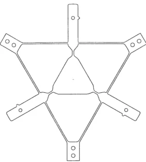
The HexflexT M_{, pictured in Fig. 1-1, is a unique compliant spatial mechanism} developed in the Precision Systems Design and Manufacturing lab (PSDAM) at MIT in 2001. Analytic models required many days to develop and solve, yet continued

Figure 1-1: The HexflexTM positioning system

to elude sufficiently precise correlation with experimental data. Many non-intuitive effects not easily captured in simplified beam models govern the Hexflex behavior. Traditional finite element analysis yielded accurate deflections and stresses, but the remaining quantities in Table 1.2 could only be obtained through dozens of slow iterations and complex analytical work. In addition, proposed conceptual design changes demanded repeated application of the entire procedure.

It is at this point that the CoMeT concept was conceived. The seed vision was to create a tool which could be used by designers for rapid first order concept design of compliant mechanisms. The tool would be designed to integrate the experience of a designer with a powerful analysis program, thereby enabling rapid generation of novel compliant mechanisms. This marriage of experience and analytic power would occur via a GUI that allows the user to create, evaluate, modify, and re-evaluate a design in less than two minutes and with better than 10% accuracy of performance.

Although it may be appear more difficult to solve the general linear elasticity problem than to solve a specific problem, this is not entirely true. Large pieces of the work had been done before, just not as part of one integrated whole. In addition, generalized formulations may be more difficult to grasp conceptually, but

are usually much easier to implement, since the same procedure is repeated many times. Moreover, given the list of proposed conceptual changes to the Hexflex, and the promise of other compliant mechanisms to be designed in the future, the point of justified return would surely be reached. Finally, it was determined that additional benefits would be gained from employing CoMeT as a teaching tool.

Once developed, CoMeT should have considerable impact on precision engineering. MEMS, optical technology, and semiconductor manufacturing all require high precision. As discussed in Section 1.1, flexures have many intrinsic advantages that suggest their use in precision applications, but are usually difficult to analyze. If CoMeT can break the analysis barrier, help engineers acquire an intuition for compliant mechanisms, empower their creativity, and shorten the product development cycle, it can help us develop these emerging technologies faster. Put simply, CoMeT is an enabling technology for next generation technologies.

1.3

Hypothesis

The hypothesis examined in this thesis is that a program can be developed whose predictions lie within 10% of traditional FEA programs, but can be used to design flexures more effectively and in less time than it would take with current tools. Furthermore, it is worth noting whether an actual physical system matches the analytic predictions of CoMeT and traditional programs. Although hypothetical discrepancies are likely to be a function of the application, it is nonetheless instructive to analyze CoMeT in an applied environment.

The metrics we will use to evaluate success are as follows:

* The accuracy of CoMeT formulas is assessed via comparisons of CoMeT to CosmosWorks® calculations. The behavior of both single elements and a complex system, namely the HexflexTM, will be scrutinized. No compliance or stress should differ by more than 10%.

development time.

* Physical flexural hardware compliance should not differ by more than 15% from its CoMeT idealization.

1.4

Scope

Although the CoMeT concept will be highly versatile, this thesis must have finite scope. Other features may be added later, as it becomes clearer what functionality is most useful. The key to allowing retro-fits is making CoMeT sufficiently modular and adaptable. This requires well-planned programming schemes and an effort to avoid limitations that may fatally limit CoMeT in the future.

In this thesis, the continuum mechanic and kinematic analyses will be limited to the isotropic and linear regime. Anisotropic materials are fairly rare in flexure design, and the most common, Silicon, is fairly stiff and brittle. Linear means that all deflections, whether linear or angular, must be directly proportional to forces and moments on each element. Geometric nonlinearity, contact mechanics, buckling, dynamics, Coulomb friction, plasticity, creep, and strain hardening analyses are therefore excluded. I have made this decision because 95% of current compliant mechanisms can be understood to first order through linear analysis. Once a system becomes nonlinear, the existence of solutions is no longer guaranteed, responses may be path dependent, superposition no longer holds, and matrix inversions must be augmented with iterative methods. Many FEA packages exist that perform all the aforementioned calculations, and if a design is evolved to the point where second order effects demand attention, commercial software can be used.

With respect to kinematic constraints, a given node must be either completely grounded (constrained to zero linear and angular displacements) or free to satisfy force equilibrium. This decision is based on the consideration that most compliant

mechanisms would become inaccurate if they included sliding or rubbing interfaces. That said, it is still possible to obtain deformation responses in CoMeT when input

displacements are known. The procedure is explained in Sec. 2.7. Alternatively, cantilever beams may be used to approximate partial constraints.

Emphasis will remain on post analysis that fits the aforementioned framework, as well as development of an intuitive, user-friendly, convenient graphical user interface (GUI). Thereby, large rewards may be reaped from ordinary effort. Without an appropriate interface, it is difficult to see CoMeT gain widespread acceptance. Without post analysis modules, CoMeT would differ little from existing frame-based FEA programs. Chapter 3 presents the post processing modules, while Chapter 4 covers the GUI in detail.

1.5

Program Structure Overview

Input geometry, materials, connectivity Store data Advanced analysis Calculate deflections, stresses, etc.

Command Line _{Editor previe}

Data file

Analyzer Optimizer Sensitivity Motion Study Diagnosis

Core Processor

(flex.m)

Figure 1-2: Program structure overview

The basic structure of CoMeT is shown in Fig. 1-2. Arrows indicate information

flow, usually in the form of function calls and data retrieval, while each box represents a CoMeT module. The "core processor", indicated by an oval, corresponds directly to

the function flex.m. Most of Chapter 2 is devoted to the workings of flex.m, written on a general level that requires no knowledge of programming. Chapter 4 elaborates on some of the subtleties required to implement the concepts from Chapter 2 in code. Graphical user interfaces (GUIs) are the de facto standard in major modern programs, and for good reason. They offer effortless data entry, visual error recognition, intuitive interaction patterns, and aesthetic appeal. This is a natural consequence of humans' visual processing capabilities. However, GUIs can never match the flexibility of a command line interface in all regards. While common functions can usually be accelerated in a graphical environment, many more sophisticated tasks are simply best suited for a keyboard. A GUI could incorporate a host of complex functions, but would lose the benefit of simplicity. It would also tend to become so "cluttered" that the accessibility of common tools would invariably suffer.

In order to capture both the visual power of a GUI and the versatility of a command line, CoMeT is designed to interact through both. This is unusual in mainstream applications, but CoMeT is intended for academic and research environments, where demands are seemingly unsatiable. The harmonious coexistence of two such dissimilar interfaces is only possible through a strict data file protocol. However strict, the format requirements are nonetheless simple and intuitive.

As shown in Fig. 1-2, both the GUI editor and the command line may read and write to this common data file. The interfaces may take arbitrary turns modifying the data. The file contains all the information necessary to define a structure study -geometry, material properties, connectivity, loading conditions, motion constraints, and points of special interest henceforth known as centroids. The command line may call the core processor directly, receiving the system deformation response, stress distribution, and other information. Thereby, data interfaces seamlessly into other MATLAB® toolboxes, custom scripts of the user's choosing, or, in textual form, foreign software (such as Microsoftg ExcelTM, PowerPointTM, or LabviewT M).

The GUI editor may also call the core processor when in instant preview mode, but usually will pass the data file information directly to an advanced analysis

module. These modules include the analyzer, the optimizer, a sensitivity study, and a motion diagnosis tool. Each calls the core processor repeatedly, capitalizing on the computational speed of flex. m. Advanced modules are discussed in Chapter 3.

Chapter 2

Continuum Mechanics and

Kinematics

The strictly linear analysis in this thesis is based on the direct stiffness approach described by Gurley [13] and others [8, 9]. Energy methods and other approaches may prove valuable when nonlinearities are considered, but remain inherently more complicated for the task at hand. Castiglione's Theorem, for example, requires partial differentiation, which is difficult to implement in code. Instead, a system of coupled linear equations, embodied in the global stiffness matrix KG, can be constructed systematically, and solving them is a simple matter of calling a built-in matrix inversion routine.

There are several more computationally efficient alternatives to explicitly inverting the global stiffness matrix, such as left division or wavefront propagation [8]. However, since a typical compliant mechanism of medium complexity may contain on the order of 100 degrees of freedom (DOF), inversion is not nearly as problematic as it would be for a finely meshed finite element model, where the number of DOF is typically three orders of magnitude higher. In addition, the possibility of defining rigid plates further reduces the DOF in KG. When inverted, KG becomes the global compliance matrix CG. It contains all the information necessary to compute deflections of every

node for any nodal load set. Clearly this is inappropriate for common FEA programs, which compute the response to one loading case at a time. In summary, computing

CG is equivalent to finding every possible forcing response in one operation.

MATLAB inverts quite efficiently by taking advantage of the fact that KG is sparse and symmetric positive definite (SPD). In practice, inversion of a typical compliant mechanism takes less than 3ms on a 1.9GHz computer. The entire analysis of the same structure took 60ms (UPDATE WHEN DONE!), which is faster than a typical human reflex. As Moore's law continues to govern the progress of computing power, the computational delay of solving the deformation response of a structure should become unnoticeable in the immediate future.

2.1

Direct Stiffness Approach

As long as deflections are small and material does not yield, as discussed in Sec. 1.4, finite elements can be represented by some linear stiffness matrix:

Fe = Kt xt (2.1)

The subscript f denotes a frame local to the element. Subsequently, g will signify quantities in the global frame pertaining to a given element, and G will represent global quantities for the entire structure. Note that Kt must be SPD [14], as dictated by the principle of reciprocal forces and the first law of thermodynamics.

The transformation matrix To/1 , covered in detail in Sec. 2.2, serves as a bridge

between local and global frames. In Eq. (2.15), To/1 is a [6x6] matrix, but in this

context the size of To/1 would reflect the degrees of freedom of the element it was

transforming (the elements used in CoMeT, with the exception of rigid plates, each have 12 DOF). Local and global generalized displacements - vectors containing linear

and angular deflections of an element's nodes - are related as follows:

xg = ToT xe

xg = T -T, xt

(2.2) (2.3)

Generalized forces - vectors combining forces and moments at element nodes -obey similar relations:

Fe = _{To-T Fg} Fg = To/, Fe

(2.4) (2.5)

We can combine Eqns (2.1), (2.2), and (2.4) to obtain

Fg = To1IKe TT₁ Xg (2.6)

If we define

Kg = To/1 KT Ti, (2.7)

Eq. (2.6) becomes

Fg = _{Kg Xg.} (2.8)

Kg will also be SPD, since TO1 is purely real (i.e. it has no imaginary or complex

components). Next, we assemble the global structural stiffness matrix KG. from element stiffness matrices Kg,i by summing over all beams,

B

KG. = Kg,i, i:=1

(2.9)

where Kg,i must be written into the appropriate fields of KG0. If beam i connects

k

k

Figure 2-1: Regions of KG. affected by addition of Kg,i

Since each addition is symmetrically placed, KG. is also SPD. We can now say

FG. =KG. XG. - (2.10)

Every node in the structure is either grounded or free. Grounded nodes have zero generalized displacements, and the loads acting on free nodes must be specified. (Since the majority of nodes will not be loaded, most applied forces and moments will be set to zero, which constitutes an easily overlooked constraint.) Therefore, we have a complete set of equations that can be solved for all unknown quantities.

If grounded nodes are listed last, Eq. (2.10) can be written in block form, k denoting known quantities, u unknown:

Fk

FU

K[ u K O x

KUU Kuo 0

I

(2.11)

For now, only Kku matters. In fact, although the element-level components of Kuu are necessary for force recovery (section 2.3), Kuu need not be constructed. Considering Eq. (2.12) a definition for Eq. (2.13), we can parallel the elegant notation of Eq. (2.6):

Fk - Kku xu (2.12)

FG - KG XG (2.13)

In the program, the summation in Eq. (2.9) simply ignores entries pertaining to

grounded nodes, and KG is created directly.

Since KG is SPD, its inverse, the global compliance matrix CG, must exist.

XG = CG FG (2.14)

Thus, the quasi-static deformation response of any loaded structure can be found.

2.2

Transformation Matrices

Transformation matrices are an integral component of CoMeT. Hale and Slocum [14]

present an excellent explanation of what they are and how they are constructed. Transformation matrices are best understood as entities that transform vectors from

a local frame to a base frame. If the base frame is numbered 0, and the local frame given the label 1, the subscript notation in TO1 suggests which frame should properly

be written on either side of the matrix. This can be seen in Eq. (2.5) and more conspicuously in later equations such as (2.128), where internal subscripts tend to

"cancel" as in Einstein notation. As to the mechanics of constructing TO1 , a summary

of Hale and Slocum's explanation follows.

To/, =oi (2.15)

C (ro) RO11 Ro/1

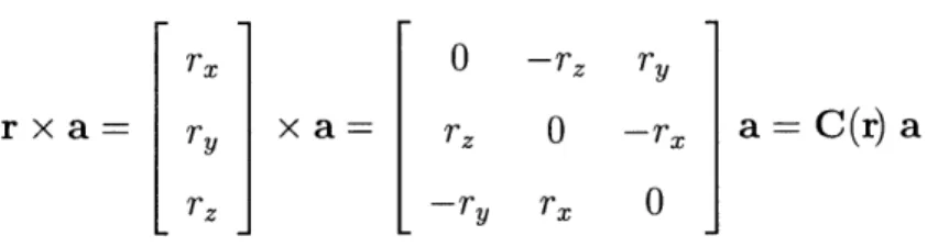
C (ro) is just a cross product matrix of the vector ro, which points from the origin of 0 to that of 1. Breaking r into (global) components and letting it act upon an

arbitrary vector a,

rX 0 - r, ry

rxa= ry xa= rZ 0 -rx a =C(r)a (2.16)

rZ -rY rx 0

Ro/i is a standard [3x3] rotation matrix that accounts for the difference in angular orientation between coordinate systems 0 and 1. There are many ways to define a rotation matrix; here, the xyz-convention is used.

Ro/1 = Rz(Oz) Ry(Oy) Rx(Ox) (2.17)

1 0 0

Rx(Ox) = 0 cosOx -sinOx (2.18)

0 sin Ox cos Ox

cos O _{0 sin,}

1

RY (0) = 0 1 0 (2.19)

L -sinO0 0 cos,

J

cosO0 -sinOz 0

R (Oz) = sin Oz cos 0, 0 (2.20)

0 0 1

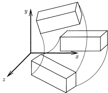
One advantage of the xyz-convention is that if 02, the angular orientation of an element throughout its volume, is zero, the top face of the element will continue to appear as a line when projected to the global xy-plane. For example, a structure extruded from an outline in the xy-plane would have all Ox set to zero. For more complex structures, the user need only determine how far beams are rotated beyond this default orientation. The xyz-convention minimizes the inherent difficulty of three dimensional visualization by decoupling O, rotations from the remaining transformations.

y

z

Figure 2-2: Beam with Ox = 0 transformed by TO1

remain parallel when Ox = 0.

While the user must specify Ox, element node coordinates determine 1, Os, and Oz. Let Ar represent coordinate offsets. In this context, 1 and 2 refer to the left and right nodes of an element, respectively.

[

Ary _{- Ty,1}

Arz rz,2 rz,1

I

(2.21)

The length of the beam can be determined from theorem.

the three dimensional pythagorean

1= Arx2 +A ry2 +Ar 2_.

The Oz relation, illustrated in Fig. 2-3, is

Oz = atan2(Arx, Ary)

(2.22)

Here 'atan2' can be considered MATLAB syntax. The atan2 command finds the polar angle of (x, y), retaining quadrant information.

y

Oz

ryr

X

/\

Figure 2-3: Oz-rotation of finite element

r/ 1

T' _X

(r, 0, rT)

z

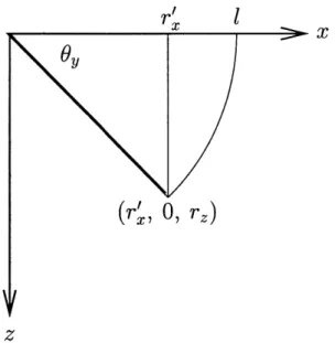
Figure 2-4:

Qy-rotation

O, is more difficult. As seen in Figures 2-3 and 2-4, r' is the intermediate x coordinate that the beam must rotate to after its Oy-rotation. At this point in time,

the beam will lie in the xz plane. Then, Oz rotates the beam to its final position.

r' = 4 (2.24)

cos(O2)

Y, atan2( 7r, rz) (2.25)

All O's are now fully defined, and can be plugged into the unit rotation equa-tions (2.18) - (2.20) to complete the transformation matrix.

2.3

Force Recovery

Once nodal displacements are known, the internal structure element forces and moments can easily be constructed. By combining Eqns. (2.1) and (2.2), we have an expression for a beam's local forces in terms of its global displacements:

Fe = Ke T 1 Xg (2.26)

First we find displacements in local coordinates:

x1 T _[0/ Ti 0

1 Fg,

(2.27)

X2 _{0 Tx/1 Xg,2 _}

Using a [12x1] matrix to represent beam forces as in Eq. (2.30) would be redundant, since beams must be in static equilibrium. It suffices to only retain the second row:

F 2]= K21 K2 2 ]. (2.28)

2.4

Element Models

The element stiffness matrix alluded to in Eq. (2.1) contains all the information necessary to describe an arbitrary body, connected to some number of nodes, with a linear elastic stiffness response. Since the script is written for three dimensional space, each node will have six DOF - three translational and three rotational DOF. All beam elements modelled in CoMeT connect two nodes, so Ke must be a [12x12] matrix. For a uniform beam with length 1, Young's modulus E, shear modulus G, cross sectional area A, torsional moment of inertia J, and area moments of inertia

I, and I, for x-z and x-y plane rotations, respectively, the complete element stiffness

matrix, if shear deflections are ignored, turns out to be:

EA 0 0 0 0 0 0A 0 12aE 0 0 0 E1 0 0 0 0 0 0 0 0 0 6-0 0 0 17E 0 0 0 0 0 0 0 0 0 GJ 0 0 0 0 0 GJ -- F 0 0 0 0 6E1 0 4EIy 0 0 0 6EIy 0 2EIy 0 0 0E1 0 0 0 4EI 0 -01 0 0 0 2EIz 0 12E 0 0 0 -% 2 EA 0 0 0 0 0 EA 0 0 0 0 0 0 "2 EI 0 0 0

We can represent Eq. (2.29) in block form as follows:

F1 F₂

I

I

ja

Ji

0

0

0

Each column can be thought of as the end node loads required to create unit F2 1 Fy1 M1 My MZi Fx2 Fy2 Fz2 Mx2 My2 Mz2_ x₁ Yi z₁ X21 0 y1 OZ1 Y2 0x2 0 y2 0z2

displacements in each DOF (corresponding to that column). For example, to stretch node 2 one unit in x (column 7) , node 1 needs to be pulled left with magnitude E,

while node 2 needs to be pulled right with the same force.

Luckily for the author, the entire [12x12] stiffness matrix need not be constructed analytically for each beam type. Since each beam must be in mechanical equilibrium under any loading condition, the upper half of the matrix depends on the lower half as follows: K _{1 2}

K

Here, T, is a 6x6 transformation matrix that expresses the stiffness at node 2 in the frame of node 1. Since both nodes have the same angular orientation, it just represents an x-translation of magnitude I (see section 2.2 for details):

T, = 1 0 0 0 0 0 0 1 0 0 0 1 0 0 1 0 -l 0 0 0 0 1 0 0 0 0 0 0 1 0 0 0 0 0 0 1 (2.33)

We also know from symmetry that

(2.34)

which can be shown to be equivalent to the statement that solid body motion does not induce internal forces. So the entire stiffness matrix can rapidly be computed once one of the block stiffnesses is known. K2 2 is the most intuitive block to work with,

since it represents the forces required at node 2 to induce unit motions at node 2, while node 1 can be thought of as grounded.

One more step remains. The "natural" beam deflections one can compute are compliance relations - given a unit force, how does the cantilever beam deflect? The responses to each unit force can be assembled into a compliance matrix, and

K2 2 = C2 (2.35)

Although K2 2 happens to have a concise analytic form in Eq. (2.29), it does not simplify as well in more general cases, including every case to follow.

In summary, we can compute the entire element stiffness matrix for any beam once deflections under various cantilever loading conditions are determined.

2.4.1

Rectangular Beams

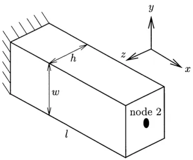
y

Figure 2-5: Uniform rectangular beam geometry

Rectangular beams, as pictured in Fig. 2-5, are the simplest and most common flexural elements. Since their tensional compliance is typically orders of magnitude smaller than their bending compliance, they provide physically compact constraints

to motion along their length. In addition, the height to width aspect ratio of a beam strongly affects its ratio of in-plane to out-of-plane bending compliance, giving a flexure designer the power to readily achieve desired characteristics. Finally, rectangular beams are usually easy to manufacture by virtue of their simple geometry. Equation (2.29) already specifies the solution for a straight rectangular beam, with

A =h-w (2.36)

1y - L wh3 (2.37)

I -=L hw3 (2.38)

Courtesy of Young and Budynas [17, p. 401], the torsional moment of inertia is

J = ab3{16 -3.36 1 - 4 (2.39)

with a and b the half-height and half-width such that a > b.

However, Eq. (2.29) neglects shear deformations, nor does it fit within the framework of the system.

Although seldom emphasized in the engineering curriculum, beams deflect under shear loading, in addition to moment bending. The longer a beam, the less significant the effect, but the critical length that determines if shear can be ignored is not always as short as one might suppose. According to Dowling [11], shear deflection for cross-sectionally symmetric beams may be quantified as follows:

6 VL (2.40)

GA

Eq. (2.40) is:

6(X) = dx' (2.41)

fo G A

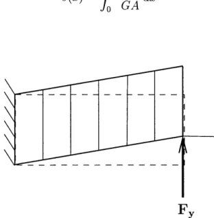
Fy

Figure 2-6: Shear deflection mode for a uniform beam

The shear deflection mode is depicted in Figure 2-6. Note that deflection varies linearly with x. Also, although the slope of the upper beam surface is certainly no longer zero, there is no rotation associated with shear. Naturally, shear deflections never occur without moment deflections, since shear is integrated to obtain the moment distribution in a beam.

Since shear deflections are linear, they may be superposed with bending deforma-tions to obtain total deflection (now specializing to loading in the y and z directions):

Fyi3 Fyl y = + G (2.42) 3EIz GA Fil3 Fil z = + -(2.43) 3EI GA

Let us take a moment to discuss the significance of shear deflections. The ratio of shear to bending deflection expresses this quantity in dimensionless form.

6

shear _ 3EI _(2.44)

6

Poisson's ratio relates E to G:

- _{= 2(1 + v)}

G

For a rectangular beam, Eq. (2.44) reduces to

6shear

6

bending rectangular

1+v (h )2

= -L (2.46)

while a round beam (using Eqns (2.50) and (2.52)) becomes

6shear 6bending round

3(1+v) h 2

-L (2.47)

Although correct, Eqns (2.46) and (2.47) do not represent a worst-case scenario. Boundary conditions may exacerbate the effect of shear. For example, the "free but guided" configuration, common in flexures as pictured in Figure 2-7, deflects significantly more when shear is accounted for. This is because slope conditions

"stiffen" the bending mode but have no effect on shear.

-

---Figure 2-7: Deformation of a parallel beam configuration

If the beams in Figure 2-7 are rectangular, the equivalent of Eq. (2.44) is

6shear

6

bending free but guided

2 ( ,,)

2

Shear deflection in Eq. (2.48) is four times greater than in Eq. (2.46) for a given bending deflection. Figure 2-8: Beam 6 shear bending 1 0.9 0.8 0.7 0.6 0.5 0.4 0.3 0.2 0.1 0 aspect ratio vs. 2

shear to bend deflection ratio

L h

3 4 5

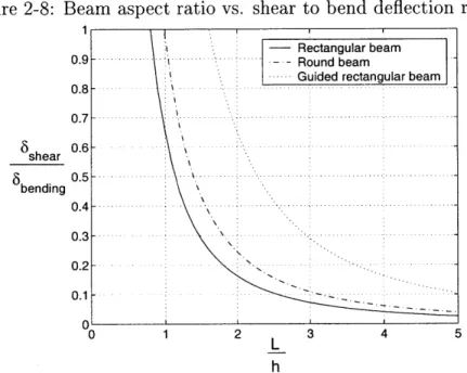
Figure 2-8 graphs Eqns (2.46), (2.47), and (2.48) as a function of the beam aspect

ratio for v = 0.3. Select values of these functions, for the same value of v, are tabulated in Table 2.1.

Table 2.1: Beam aspect ratio

(Q)

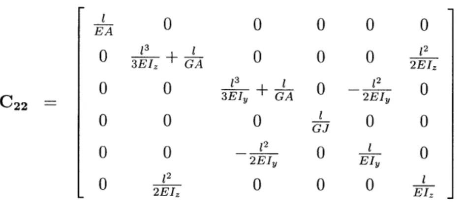
Combining Eqns (2.42), (2.43), and the standard cantilever beam equations, we (2.48)

Rectangular beam

- Round beam

Guided rectangular beam -. ...- ... ..................... ---. ... -..--.-.-.-6_shear/6 bend 100% 10% 5% 1% Rectangular 0.80 2.55 3.61 8.06 Round 0.99 3.12 4.42 9.87 Guided 1.61 5.10 7.21 16.1 1

can construct the compliance matrix: 1 0 0 0 0 0 0 _3EI 13+ _GA 0 0 0 _2EI1 C - 0 0 13+ 1 0 12 0 C2 2 -- 0 I 2EIY (2.49) 0 0 0 G 0 0 0

_o

The matrix is SPD, and x-y planar motion (x, y, 0,) is de-coupled from out-of-plane forcing and vice-versa.

2.4.2

Round Beams

y

Ax

h

node 2

Figure 2-9: Uniform round beam geometry

Round beams, pictured in Fig 2-9, are also fairly common structural elements. They are often easy to manufacture, depending on the field of application. Circular beams have the property that each outer fiber is stressed by the same amount