The informational value of environmental taxes *

HAL Id: hal-02945523

https://hal.inrae.fr/hal-02945523

Preprint submitted on 22 Sep 2020

HAL is a multi-disciplinary open access archive for the deposit and dissemination of sci-entific research documents, whether they are pub-lished or not. The documents may come from teaching and research institutions in France or abroad, or from public or private research centers.

L’archive ouverte pluridisciplinaire HAL, est destinée au dépôt et à la diffusion de documents scientifiques de niveau recherche, publiés ou non, émanant des établissements d’enseignement et de recherche français ou étrangers, des laboratoires publics ou privés.

The informational value of environmental taxes *

Stefan Ambec, Jessica Coria

To cite this version:

The informational value of environmental taxes

∗

Stefan Ambec

and Jessica Coria

January 2020

Abstract

We propose informational spillovers as a new rationale for the use of multiple policy instruments to mitigate a single externality. We investigate the design of a pollution standard when the firms’ abatement costs are unknown and emissions are taxed. A firm might abate pollution beyond what is required by the standard by equalizing its marginal abatement costs to the tax rate, thereby revealing information about its abatement cost. We analyze how a regulator can take advantage of this information to design the standard. In a dynamic setting, the regulator relaxes the initial standard in order to induce more information revelation, which would allow her to set a standard closer to the first best in the second period. Updating standards, though, generates a ratchet effect since the low-cost firms might strategically hide their cost by abating no more than required by the standard. We provide conditions for the separating equilibrium to hold when firms act strategically. We illustrate our theoretical results with the case of NOx regulation in Sweden. We find evidence that the firms that are

taxed experience more frequent standard updates.

Keywords: pollution, externalities, asymmetric information, environmental regulation, tax, standards, multiple policies, ratchet effect, nitrogen oxides.

JEL codes: D04, D21, H23, L51, Q48, Q58.

∗_{We thank the participants at various conferences and seminars for useful feedback. This research}

was supported by the TSE Energy and Climate Center, the H2020-MSCA-RISE project GEMCLIME-2020 GA No. 681228, the ANR under grant ANR-17-EURE-0010 (Investissements d’Avenir program) and the Swedish Foundation for Humanities and Social Sciences (Riksbankens Jubileumsfond).

†_{Toulouse School of Economics, INRAE, University of Toulouse Capitol, 1 Esplanade de}

l’Universit´e, 31000 Toulouse, France, and University of Gothenburg. Email: stefan.ambec@inra.fr. Phone: +33 5 61 12 85 16. Fax: +33 5 61 12 85 20.

1

Introduction

The economic literature traditionally argues for the superiority of market-based policy instruments over command-and-control regulation, primarily because of the relative cost savings expected with market-based approaches. In practice, the laws pertaining to many major environmental problems, as for instance, clean air, clean water and management of hazardous waste - are typically enacted and managed at all levels of government, implying that many regulations covering the same emission sources overlap and override each other. This is, for instance, the case of climate policy, where all countries and regions that have implemented climate policies seem to rely on several policy instruments (covering the same emission sources) rather than a single one (see e.g., Fankhauser et al. 2010, Levinson 2011 and Novan 2017).

The multiplicity of policy instruments to address a single pollution problem has been justified on several grounds. For instance, some (additional) market failures, regulatory failures or behavioral failures may reduce the economic efficiency of market-based instruments and justify additional policy instruments (see e.g., Bennear and Stavins 2007, Lehmann 2012, Lecuyer and Quirion 2013, Coria et al. 2018). The aim of this paper is not to discuss these justifications, but to introduce and discuss another rationale: the informational value of the policy overlap. In particular, we highlight the informational value of a pollution tax in the design of other environmental regulations when the firm’s costs of abating pollution are unknown. We investigate whether and how a tax can help regulators set and update a standard (a cap) on pollutant emissions. Our idea is that the tax rate reveals information about the marginal cost of compliance that can be used to better target the standard to the firm’s true cost.

The empirical motivation behind our paper is the regulation of NOx emissions by

stationary pollution sources in Sweden. Since NOx causes environmental damages at

both a national and local level, it is regulated through a combination of a nationally determined emission tax and locally negotiated emission standards which are revised over time. The level of the tax has remained stable since its implementation, although not all pollution sources are taxed. We investigate how taxing emissions has modified emission standards. Does taxing polluters result in more or less stringent local stan-dards? How does the standard evolve over time with and without tax? To answer these questions, we develop a theoretical analysis of the design of an emission standard by a welfare-maximizing regulator under asymmetric information about abatement costs, with a tax on emissions which is set exogenously (i.e. out of the control of the reg-ulator). We highlight the informational spillover that the tax induces on the design

of the standard over time. We then take advantage of the regulatory heterogeneity between stationary pollution sources in Sweden to investigate the extent to which this informational spillover has been used in the design of NOx standards at the county

level.

To the best of our knowledge, this is the first study investigating the informational value of an economic instrument (a tax) for the design of a command-and-control in-strument (a standard). Previous studies have analyzed the effectiveness of multiple instruments when there is uncertainty about abatement costs. Building on Weitzman (1974), Roberts and Spence (1976) show, for instance, that a mixed system, involving taxes and quantity regulations (in the form of marketable tradable permits) is prefer-able to either instrument used separately because such a mix better approximates the shape of the pollution damage function. A similar argument is developed by Mandell (2008) and Caillaud and Demange (2017), who show that, under some conditions, it is more efficient to regulate a part of emissions by a cap-and-trade program and the rest by an emission tax, rather than using a single instrument. Another strand of the literature has taken a mechanism design approach to analyze environmental regulation when abatement costs are unknown by the regulator, e.g., Kwerel (1977), Dasgupta, Hammond, and Maskin (1980), Spulber (1988), Lewis (1996), Duggan and Roberts (2002). Those studies rely on the direct revelation mechanism to identify a regula-tion that induces truthful revelaregula-tion of abatement costs. They end up recommending complex instruments, such as non-linear pollution taxes. Our approach is different in the sense that we do not look at the design of an individual instrument to induce in-formation revelation. We indeed take it as given: the environmental tax is exogenous to the regulator. The question is rather how the regulator can take advantage of the information revealed by the tax to set correctly another instrument which does not reveal information. We thus show that a local regulator can make use of the informa-tional properties of a market-based instrument to ensure local air quality at a lowest cost with a command-and-control instrument. It is so even if the market-based instru-ment is exogenous for the regulator because it is controlled by another administration, potentially at higher level, e.g. national or federal.

The dynamic design of regulation with information revelation leads to the well-known ratchet effect that has been studied in contract theory but seldom investigated in the context of environmental policies. Previous theoretical analysis has shown that the ratchet effect precludes information revelation, often leading to pooling and semi-pooling equilibria (Freixas, Guesnerie and Tirole, 1985, Laffont and Tirole, 1988). In

our framework, we identify under which conditions the separating equilibrium survives the ratchet effect and how much information is revealed. Furthermore, we show that a higher tax level improves information revelation, and that this effect remains despite the ratchet effect.

The paper is organized as follows. Section 2 motivates our research question based on actual regulation in Sweden. Section 3 introduces the theoretical model. Sections 4 and 5 analyze the choice of emission standard under pooling and separating equilibrium, discussing how the level of the tax can be used to induce revelation of information in a static and dynamic setting, respectively. Section 6 generalizes the results when firms take into account the effect of information revelation on the update of stringency of the regulation. Section 7 illustrates the theoretical analysis in a two-types framework. Section 8 revisits NOxregulation in Sweden in light of our theoretical analysis. Finally,

Section 9 concludes the paper.

2

Empirical Background

For geological reasons, Sweden is particularly vulnerable to acidification, causing neg-ative impacts on lake and forest ecosystems. Consequently, NOx emissions have been

an important environmental policy target in Sweden. Combustion plants are subject to a heavy NOx national tax and most (but not all) are also subject to individual NOx

emissions standards specified in operating licenses issued case-by-case, either by one of the 21 regional County Administrative Boards, or by one of the five Environmental Courts that cover a geographical area of several counties.1 _{Important legislative}

frame-works that the County Administrative Boards must consider in the determination of NOx emission standards are some EU directives and the Swedish Environmental Code.

If motivated, the regional decision maker can impose more stringent standards than the minimum requirements specified in these directives. These should be determined in line with the Environmental Code which, for example, states that regulations should be based on what is environmentally desirable, technically possible and economically reasonable.

NOxemissions standards at the production plant level were introduced in the 1980s.

There is no legal limit for how long a standard specified in an operating license is valid, though the common practice seems to be that operating licenses and standards are

re-1_{After the first of June 2012, only 12 County Administrative Boards, instead of 21, are responsible}

vised no latter than every tenth year. Firms must, however, apply for a new operating license if they make large changes to the operations (e.g. installing a new boiler or retrofitting a boiler to use a different type of fuel). In addition, there can be appeals that change the original permissions, or postpone conditions for operation. In the ap-plication, firms are required to submit information about the operations at the plant and they can propose emission standards based on evidence. However, each County Administrative Board considers whether the suggested emission standards are reason-able. Standard are boiler-specific so that similar firms might end up with different standards assigned to their boilers within the same juridiction. In order not to dis-tort competitiveness, they usually compare emission standards of boilers with similar characteristics in terms of, for example, size and sector classification. If a firm violates the standard specified in the operating license, it risks criminal charges and could face fines to be determined in court.

Regarding the Swedish tax on NOx emissions from large combustion plants, at

the time it was introduced in 1992, close to 25% of the Swedish NOx emissions came

from stationary combustion plants and the tax was seen as a faster and more cost-efficient way of reducing NOx emissions than the already existing standards. The

installation of measuring equipment was judged too costly for smaller plants and the charge therefore was only imposed on larger boilers. In order not to distort competition between larger plants and smaller units not subjected to the tax, a scheme was designed to refund the tax revenues back to the regulated plants in proportion to energy output. Energy output is measured in terms of so-called useful energy, which can be in the form of electricity or heat depending on end-use. Regulated entities belong to the heat and power sector, the pulp and paper industry, the waste incineration sector and the chemical, wood, food and metal industries. Initially the tax only covered boilers and gas turbines with a yearly production of useful energy of at least 50 GWh, but in 1996 the threshold was lowered to 40 GWh and in 1997 further lowered to 25 GWh per year. We provide evidence that taxed and untaxed boilers are regulated differently by local authorities. We collected information about boiler specific standards for the period 1980-2012 from authorities. Using such information, we examine the evolution of standards of both types of boiler (taxed and untaxed), expressed in milligrams of NOx per MegaJoule (mg/MJ) of useful energy, before and after the tax was introduced.

We report the number of boilers and the average standards in Table 1.2 _{It turns out that}

2_{In total, 819 boilers have been subject to standards. Out of these, 240 have been exempted from}

the NOx tax while 579 have been subject to the NOx tax at least one year since 1992. Standards

the stringency of standards has increased significantly over time (about 44%, decreasing from an average of 187.05 mg/MJ before the implementation of the charge in 1992 to 104.86 mg/MJ afterward). Moreover, the increased stringency is more pronounced for the group of boilers that are charged (e.g., 48% vs 31% reduction, respectively).

Number of Standard (mg/MJ) Standard (mg/MJ) Boilers before 1992 after 1992

Taxed boilers 516 193.23 101.05

Untaxed boilers 225 165.17 113.90

Total 741 187.05 104.86

Table 1: Average standard before and after the NOx tax was introduced

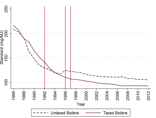
We graph the evolution of the average standard between the years 1985 and 2012 for taxed and untaxed boilers in Figure 1.

standards expressed in the same unit: milligrams of NOx per MegaJoule (mg/MJ) of useful energy.

We exclude the 78 boilers whose standards are expressed in other units. We end up with 741 boilers, out of which 516 are taxed.

Figure 1: Average Standard by Year

The average standards of the two type of boilers, those that are taxed at some point in time and those that are exempted, follow a similar trend of reduction of the emission standard over time prior to the introduction of the NOx tax in 1992, 1996 or 1997,

depending on the boiler’s annual energy use. The two lines diverge just after the tax was introduced, as taxed boilers experienced more stringent standard updates on average.

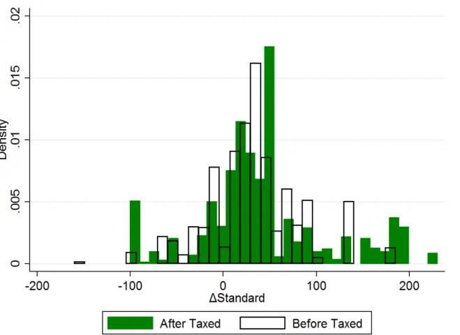
We alsoexamine how standards are updated before and after the tax has been introduced. For a given boiler, we compute the magnitude of the revision ∆Standard as the difference between the standard that applies to the boiler before and after the revision. The revision strengthens the standard when ∆Standard > 0, while it relaxes it when∆Standard < 0. In the data, about 20% of the standards of taxed boilers have been revised towards less stringent standards. In Figure 2, we plot the distribution of the magnitude of the standard revisions for the taxed boilers, separating between those revisions that took place before and after the boilers were taxed.3

Figure 2: Variations in standard stringency of taxed boilers

The figure suggests a different distribution before and after the introduction of the tax. A two-sample Kolmogorov-Smirnov test allows us to reject the null hypothesis of equality of the distributions. It seems that there is a greater spread in the magnitude of the revision in absolute values when the boilers are taxed, with a higher share of extreme values on both the positive and negative sides. This evidence is consistent with the idea that the information provided by the tax system is used by the local regulators to better tailor the standard. When updating standards, the regulator might take into account whether the boiler over-complies with current standards, and by how much; this would explain the larger variation of the update of stringency of standards for taxed boilers. We explore this explanation in a theoretical framework introduced in the next section.

the tax in 1996 or 1997. Moreover, our data is composed of an unbalanced panel where new boilers appear in the data every year. Thus, the year when a given boiler started to be taxed will depend on the year when the boiler started operating and on the boiler’s size.

3

The model

We rely on the textbook model of environmental externality with pollution abatement. Let us assume that a public authority called ‘the regulator’ (hereafter referred as ‘she’) is regulating air pollution emitted by a firm through an emission standard. The reg-ulator is a welfare-maximizer: she cares about environmental damage and the cost of controlling pollution. Emissions can be abated by the firm at some cost which is un-known by the regulator. Let q denote pollution abatement. The benefit from reducing pollution by q units is B(q) while the cost is θC(q). The parameter θ captures the level of abatement costs. It is called the firm’s type and it is exogenously given.4 _{It belongs}

to the range [θ, ¯θ] with ∆θ = ¯θ− θ > 0. The density and cumulative distribution of the a priori beliefs on the distribution of θ over the range [θ, ¯θ] are denoted f and F respectively. The benefit function B(q) is increasing and (weakly) concave, reflecting decreasing (or constant) marginal benefit from abating pollution. Similarly, the cost function C(q) is increasing and convex, thereby implying an increasing marginal cost of abating.

The welfare from having a firm of type θ abating q units of polluting emissions is:

W (q, θ)_{≡ B(q) − θC(q).} (1)

The first-best abatement level q∗_{(θ) maximizes W (q, θ) with respect to q. It is defined}

by the following first-order condition:

B′(q∗(θ)) = θC′(q∗(θ)), (2)

for every θ∈ [θ, ¯θ].

An emission standard defines a minimal abatement effort denoted s.5 _{Assume that}

pollution is regulated solely through the standard. Under uncertainty about θ, the regulator imposes a standard that maximizes the expected welfare given her beliefs about the firm’s type. Let ˆθ _{≡ E}θ[θ] be the firm’s expected type given the regulator’s 4_{The model can easily be extended to endogenize θ via the investment in new technologies at}

expenses of a fixed cost. The same argument would hold as long as the investment is profitable for the firm. If not, the standard might be strengthened further to induce this investment.

5_{Although the NO}

x standard in Sweden is a relative standard determined by units of energy

used, we consider an absolute standard (a cap) on emissions in the theoretical model to avoid adding production (energy) as another decision variable. By doing so we ignore output-based strategies to comply with the standard, such as the so-called dilution effect; see e.g. Phaneuf and Requate (2017, Chapter 5). Nevertheless, the main argument holds with relative standards.

beliefs. The ex ante efficient abatement standardqˆ∗ _{maximizes the expected welfare}

Eθ[W (q, θ)] = W (q, ˆθ) = B(q)− ˆθC(q),

with respect to q. The first-order condition that defines q∗_{(ˆθ) equalizes the marginal}

benefit from abatement to the expected marginal cost:

B′(q∗(ˆθ)) = ˆθC′(q∗(ˆθ)). (3)

Consider now a tax per unit of pollution denoted τ . It makes abatement profitable for the firms even in the absence of an emission standard because the firm saves τ each time it reduces emissions by one unit. Therefore, in absence of a standard, the firm chooses the abatement level that minimizes its cost including the tax bill saved, formally θC(q)_{− τq. Let us denote as q}τ_{(θ) the abatement effort carried out by the}

firm of type θ. It is defined by the first-order condition that equalizes the marginal abatement cost to the tax rate:

θC′(qτ(θ)) = τ. (4)

Therefore qτ_{(θ) = C}′−1!τ

θ "

for every θ. It is increasing with the tax rate τ and decreasing with the type θ.

We analyze the design of a standard s with an exogenous tax on emissions. We assume that the tax does not fully internalize the benefit of abatement. This is to say, the abatement level induced by the tax is sub-optimal regardless of the type: qτ_{(θ) < q}∗_{(θ) for every θ.}6

The regulation game is the non-cooperative game aiming at modeling the relation-ship between the regulator setting the standard and the firm. The tax is exogenous to the two players and common-knowledge. The game is played under adverse selection since the firm observes its type θ before choosing its abatement strategy. The regulator sets the standard s before the firm chooses its abatement effort q. We first consider a static version of the game played only once. We then extend it to two periods to investigate standard revision with information acquisition.

6_{This assumption implies that standards are set for all firm types. It avoids considering the case of}

over-abatement with tax compared to the optimal level. This can easily be justified empirically since most environmental taxes are set below the Pigouvian rate. It is also theoretically grounded because the national tax should reflect only part of the marginal damages due to a boiler’s polluting emissions: the part that is not internalized at the county level from the emissions that exit the county’s borders.

4

The tax as a separating device

4.1

The pooling and separating solutions

We solve the static regulation game by backward induction. Given the abatement standard s, the firm chooses its abatement effort that minimizes its cost subject to complying with the standard. The firm of type θ chooses q that minimizes θC(q)− τq subject to q _{≥ s. If the constraint is not binding, the tax rate drives the firm’s} abatement effort and the firm equalizes marginal abatement cost to the tax rate by choosing the abatement level qτ_{(θ), defined in (4). Otherwise, the firm’s abatement}

effort matches the standard s. Thus, firm θ’s best reply to the standard s defines an incentive-compatibility (IC) constraint:

q(θ) = max_{{s, q}τ(θ)_}. (5)

The regulator chooses the standard s that maximizes the expected welfare E[W (q(θ), θ)] = E[B(q(θ))_{− θC(q(θ))] subject to the firm’s IC constraint (}5).

For low tax rates, the tax is not binding and the solution is pooling as all types abate at the standard level. The abatement level qτ_{(θ) is so low that the IC constraint}

simplifies to q(θ) = s for every θ. The standard is set at the first-best level for the mean type ˆθ, i.e., s = q∗(ˆθ). For higher tax rates and a given standard s, the IC constraint defines a threshold ˜θ such that q(θ) = qτ_{(θ) if θ ≤ ˜θ and q(θ) = s if θ ≥ ˜θ. This is to}

say, firms with a type θ below the threshold abate a level determined by the tax while firms with a type θ above the threshold abate what is required by the standard. The threshold is defined by qτ_{(˜θ) = s or, equivalently, by ˜θ =} τ

C′(s). Hence, the regulator chooses the standard s to maximize:

max s # _θ˜ θ W (qτ(θ), θ)dF (θ) + # _θ¯ ˜ θ W (s, θ)dF (θ) subject to qτ(˜θ) = s.

Let us denote the standard that solves this problem as ss _{(with an upper-script ‘s’ for}

static). The first-order condition yields:

B′(ss)[1− F (˜θ)] = # θ

˜ θ

Using the Bayes rule f(θ|θ ≥ ˜θ) = f (θ)

1− F (˜θ) leads to

B′(ss) = E[θ|θ ≥ ˜θ]C′(ss), (6) In the separating solution, the standard is chosen such that the marginal benefit of abatement equals the marginal cost in expectation for all types for which the standard is binding, i.e, with a θ higher than ˜θ.7

4.2

More information revealed with higher taxes

We now examine how the standard varies with the tax rate.8 _{First, the tax rate}

determines whether the solution is pooling or separating. The solution is separating if the tax rate is higher than a threshold defined by the marginal abatement cost of the lowest-cost type firm θ with the pooling standard q∗_{(ˆθ). That is, if q}τ_{(θ) > q}∗_(ˆθ).

Using (4), this leads to τ > θC′_(q∗_(ˆθ)).

Second, a tax increase has two effects on type revelation in the separating solution. The first one is a direct positive effect as higher tax rates induce more revelation of types, since the threshold ˜θ for which the tax determines abatement increases with τ . Indeed, using the definition of ˜θ, we obtain d_dτθ˜ = 1

C′(s) > 0, implying that more types are revealed with higher taxes for a given standard s. The second effect is indirect and negative because a higher tax makes the standard more stringent, which reduces ˜θ for a given tax rate. By differentiating (6) with respect to τ , we observe that

ds dτ =−

C′(ss)

B′′(ss)_{− E[θ|θ ≥ ˜θ]C}′′(ss) > 0

implying that a higher tax increases the standard which, because dθ˜ ds =−˜θ

C′′(s) C′(s) < 0, reduces the threshold type ˜θ and, thus, it reduces revelation of types. We show in Appendix A that the net effect is positive: more types are revealed when the tax increases.

We close this section by summarizing our finding in the following proposition. Proposition 1 In the static setting in which the firm is regulated both by a standard and a tax, the firms reveals its type by over-complying with the standard when its

7_{Note that our assumption q}∗_{(θ) > q}τ_{(θ) implies that the standard is binding for some types}

because ˜θ > θ.

abatement cost is low. The standard is more stringent and more types are revealed with higher taxes.

As mentioned in Section 1, previous studies (see e.g., Roberts and Spence, 1976, and Pizer, 2002) have shown that using multiple instruments to regulate the same pool of polluters can be welfare enhancing when there is uncertainty about abatement costs. For instance, using an initial distribution of tradable emission permits to set a quanti-tative target on emissions abatement but allowing for a price cap can be a cost-efficient alternative to either a pure price or quantity system. Proposition 1 is in line with such a result in the sense that a combination of quantity and price control provide firms with greater flexibility to choose the level of emissions abatement closer to the optimal. Nevertheless, the previous studies have ignored another benefit from using multiple instruments: the information revealed about abatement costs. We now investigate how the regulator can make use of this information to improve the regulation. To do that, we need to add a new period into the regulation game. We investigate not only how the information revealed can be used to update the standard but also how it modifies the choice of the initial standard by comparing it to ss _.

5

Information revelation with a myopic firm

5.1

Regulation update

Let us assume now that the regulation game is repeated twice with a discount factor β. The type θ is observed by the firm at the beginning of the game and remains unchanged. Each period t, the regulator sets a standard st and the firm chooses the

abatement qt(θ) for t = 1, 2. We assume that the firm is myopic or short-term in its

thinking, as it considers only the current abatement costs when picking its abatement strategy. This assumption is relaxed in the next section.

The regulation game with update is a dynamic game under adverse selection. We use the concept of Perfect Bayesian Equilibrium (PBE). The equilibrium strategies are formally described in Appendix B.1. In this section, we solve the game by backward induction. Given the first-period standard s1, after having observed the firm’s

abate-ment strategy in period1, the regulator designs a new standard s2. The regulator takes

advantage of the information revealed by the firm’s abatement decision during the first period to update its beliefs on the firm’s type. Given the information obtained, she

tailors the standard closer to the firm’s expected type.9 _{If the firm was over-complying}

by abating qτ_{(θ) > s}

1, the regulator can perfectly infer that its type is θ. She updates

the standard to the first-best abatement level s2 = q∗(θ). A firm with types lower than

the threshold given by:

τ = ˜θ1C′(s1), (7)

is over-complying and, therefore, experiences a standard update s2 = q∗(θ). If the firm

was only abating the level required by the standard s1, some uncertainty about its type

remains. Nevertheless the information on the firm’s type becomes more precise because types lower than ˜θ1 can be excluded. The firm’s type should therefore belong to the

range[˜θ1, ¯θ]. It is distributed according to the conditional cumulative F (θ|θ ≥ ˜θ1).

The updated standard s2 maximizes the expected welfare given the updated beliefs:

E[B(q2(θ))− θC(q(θ))|θ ≥ ˜θ1] subject to q2(θ) = max{s2, qτ(θ)} (8)

The program is similar to that in the static model with the updated beliefs. Let’s call V (s2, ˜θ1) the maximal value of (8) given ˜θ1, i.e.

V (s2, ˜θ1)≡ max s2

E[W (q2(θ), θ)|θ ≥ ˜θ1] subject to q2(θ) = max{s2, qτ(θ)}.

Let us denote sd

2 the solution to problem (8). In what follows, we discuss the optimal

choice of the standards in each period.

5.2

First period’s standard

In the first period, the regulator chooses the standard s1that maximizes the discounted

expected welfare given that the standard will be updated to s2 = q∗(θ) if the firm abates

more than s1 and to the standard s2 = sd2 if the firm abates s1. The regulator thus

maximizes: # _θ˜₁ θ W (qτ(θ), θ)dF (θ)+ # _θ¯ ˜ θ1 W (s1, θ)dF (θ)+β $# _θ˜₁ θ₁ W (q∗(θ), θ)dF (θ) + V (sd₂, ˜θ1) % (9)

9_{We focus on the separating solution because no new information is revealed if the solution is}

where ˜θ1 is defined in (7) with θ < ˜θ1 < ¯θ. The last term in the brackets in (9)

is the second-period welfare in expectation. It includes two terms: (i) the first-best welfare W(q∗(θ), θ) for firm types θ ≤ ˜θ1 that revealed their type by over-complying,

and (ii) the maximal value of the expected welfare with the revised standard s2 given

the updated beliefs that the firm is of types θ≥ ˜θ1.

The solution to the problem (9) denoted sd

1 satisfies the following first-order

condi-tion: B′(sd₁) = E[θ|θ ≥ ˜θ1]C′(sd1)−β & W (q∗(˜θ1), ˜θ1)− W (q2(˜θ1), ˜θ1) ' ( )* +

Welfare gain from revealing ˜θ1

f (˜θ1|θ ≥ ˜θ1) d˜θ1 ds1 , (10) where dθ˜1 ds1 = −˜θ1 C′′(sd 1)

C′(sd₁) < 0 is found by differentiating (7) and q2(˜θ1) is the firm ˜θ1’s abatement level during the second period. The standard sd

1 is such that the marginal

benefit of a more stringent standard on the left-hand side of (10) equals the marginal cost on the right-hand side. Likewise for the first-order condition of the static prob-lem in (6), the marginal cost is computed in expectation over all types for which the standard is binding, i.e., all θ higher than ˜θ1. What is new compared to (6) is the

second term on the right-hand side that accounts for the marginal value of the in-formation revealed by the tax. This value is the marginal loss of welfare from not revealing types with a more stringent standard. It is decomposed into three terms. First, dθ˜1

ds1 < 0 captures the fact that increasing s1 decreases the threshold type ˜θ1,

which means that fewer firm’s types are revealed. Second, the difference in the brack-ets W !q∗_(˜θ

1), ˜θ1

"

− W!q2(˜θ1), ˜θ1

"

is the welfare gain of revealing the marginal type θ1 (or the welfare loss of not revealing it). Indeed, if ˜θ1 had been revealed, the

stan-dard could be set at the efficient level q∗_(˜θ

1) in the next period, thereby achieving the

maximal welfare W!q∗_(˜θ 1), ˜θ1

"

. Instead, the welfare level achieved is W !q2(˜θ1), ˜θ1

" , where the abatement of the firm of type ˜θ1 is determined by the second-period standard

s2.10 Third, this loss is weighted by the regulator’s updated beliefs about the share

of threshold types f(˜θ1|θ ≥ ˜θ1) and discounted with the factor β to be expressed in

first-period welfare units.

The welfare gain from revealing ˜θ1 in (10) is strictly positive, provided that q∗(˜θ1)∕=

q2(˜θ1) and β > 0. Hence the marginal loss of making the standard more stringent is 10_{We have q}

2(˜θ1) = qτ(˜θ1) if the standard is relaxed at s2< s1 or q2(˜θ1) = s2 if it is strengthened

higher in the dynamic model than in the static one, because the right-hand side of (10) is higher than the right-hand side of (6) for a given standard.11 _{Since the left-hand side}

of both conditions (6) and (10) are the same function of the standard, we have sd 1 < ss.

This is to say, the standard is relaxed to acquire information that is used next period.

5.3

Second period’s standard

Given s1 and, therefore the threshold type ˜θ1, we can now solve the second-period

maximization program V(s2, ˜θ1) that defines the second-period standard s2 if the firm

does not over-comply with the standard s1. V(s2, ˜θ1) is similar to the static problem

with updated beliefs f(θ_{|θ ≥ ˜θ}1) on the range of types [˜θ1, ¯θ]. In Appendix B.2., we

show that the second-period standard denoted sd

2 pools of all types in this range: the

threshold type is ˜θ2 = ˜θ1. The first-order condition is then:

B′(sd₂) = E[θ_{|θ ≥ ˜θ}1]C′(sd2). (11)

The above first-order condition differs from the one that defines sd

1 in (10) by the last

term in brackets in (10). It does not show up in (11) because, as the game ends, there is no future gain from revealing types. As the consequence, the standard is strengthened in the second period: sd

2 > sd1. Updating to a more stringent standard in the second

period implies q2(˜θ1) = sd2 in (10). Hence, the firm of the threshold type ˜θ1 abates

at the standard level in both periods. Thus, the welfare gain from revealing θ1 in

(10) becomes W(q∗(˜θ1, ˜θ1)− W (sd2, ˜θ1), which corresponds to the difference between

the first-best welfare and the welfare with abatement at the standard level sd

2 when the

firm is of type ˜θ1.

Proceeding as in AppendixA, one can show that a higher tax induces more revela-tion of types, i.e. a lower ˜θ1, in the dynamic regulation game.

Our results are summarized in the proposition below.

Proposition 2 In a dynamic setting in which a firm are regulated by a standard and a tax, the tax is used to reveal information about the marginal cost of abatement over time. The first-period standard is lower than in the static model to induce more revelation of types, i.e., sd

1 < ss. It is then strengthened to the first-best abatement level if the firm

reveals its type by over-complying, i.e., if q1(θ) = qτ(θ) > sd1 then s2 = q∗(θ) > sd1. It is 11_{Consistently, the first-order (10) boils down to the one of the static model (6) whenβ = 0.}

also strengthened if the firm does not overcomply with the standard, i.e., s2 = sd2 > sd1

if q1(θ) = sd1. More revelation of types is achieved with higher taxes.

Before moving to the analysis of a strategic firm, we briefly discuss how our results would change if the firm’s type changes over time. By assuming perfect correlation of type across periods, we assign a maximal value to the information revealed by the environmental tax about the abatement costs in the second period. Full information is revealed if the firm over-complies during the first period, which leads the regulator to implement the first-best. Furthermore, the regulator can exclude a full range of poten-tial types if the firm does not overcomply. In reality, a firm’s abatement costs evolve over time due to technological progress and the business environment, which means in our model that the first-period cost type is only partly correlated to the second-period one. Nevertheless, as long as the types are correlated over time, the information revealed in the first period has some value in the second period. Even though the first-best might not be achieved if the firm over-complies, welfare is improved as long as the information about the first-period type allows the regulator to reduce the variance of her beliefs about the second-period type. The standard is probably strengthened but not as much as it would be with perfect correlation. Similarly, when the firm’s abatement does not exceed the standard, the full range of potential types excluded in the first period cannot be excluded in the second period. Yet the regulator has more precise information about the firm’s type in the second period than she had initially in the first period, which allows her to modify the standard in the second period. Hence, the informational spillovers between policy instruments would remain under imperfect but positive correlation among the firms’ abatement costs across time.

6

Information revelation with a strategic firm

Let us assume now that firms are forward looking and strategic. They take into account the impact of their abatement strategy in the first period on the second period standard. The revision of the standard leads to the well-known ratchet effect in the separating equilibrium of the dynamic regulation game. As the regulator makes the standard more stringent for firms revealing their low-cost type, it induces them to hide their type by abating only the level required by the standard.

Two behaviors might prevent the revelation of types. First, the firm of type θ might hide its cost by abating at the level of the standard s1 instead of its

cost-minimizing abatement level qτ_{(θ) > s}

period. However, this extra cost can be more than offset by the future gain from a lower standard updating, as the firm the will be required to abate s2 instead of q∗(θ).

Second, firm θ might mimic a higher-cost type θ′ > θ by picking the abatement strategy qτ_(θ′_{) > s}

1 to avoid a more stringent standard update in the future, i.e. s2 = q∗(θ′)

instead of s2 = q∗(θ) with q∗(θ′) < q∗(θ). We examine these two types of opportunistic

behavior separately.12 _{They define two dynamic incentive-compatibility constraints}

ensuring truthful revelation of types with strategic firms.

Firm θ reveals its type by abating more than the standard, if the following dynamic incentive-compatible constraint holds:

θC(qτ(θ))_−τqτ(θ)+β[θC(q∗(θ))_−τq∗(θ)]_{≤ θC(s}1)−τs1+β[θC(qτ(θ))−τqτ(θ)]. (12)

The discounted cost if the type is revealed on the left-hand side of (12) should be not be higher than if it is hidden in the right-hand side. The firm has to balance the current extra cost of abating s1 instead of its cost-minimization level qτ(θ) (first two terms on

each side of the inequality), with the future benefit of being able to minimize cost by abating qτ_{(θ) instead of updated standard q}∗_{(θ) (terms in brackets on the two sides of}

the inequality), discounted in present value.13

It is possible to show that the dynamic incentive-compatible constraint for hiding the type is binding for any standard. Indeed, substituting s1 = qτ(˜θ1) into (12) shows

that this inequality does not hold. By continuity, it does not hold either for types close to ˜θ1. Hence, strategic firms undermine information revelation. However, if the cost

difference between revealing and hiding type is increasing with θ, condition (12) might hold for the lowest cost-types θ. In Appendix C.1 we define conditions for which this is indeed the case. It basically requires that the cost function C(q) is not too convex and/or the discount factor β is not too high. Under Assumption 1 in AppendixC.1, we can define ˙θ as the threshold such that (12) holds for all θ < ˙θ. Formally, ˙θ is defined

12_{Note that a firm would never mimic a lower type because it would imply abating more both}

periods.

13_{Note that if the game lasted more than two periods (i.e. the standard was updated several times),}

the firm might hide its type again in the second period to avoid the standard being updated toq∗_(θ)

later on. This reduces the benefit from hiding type in the future and, therefore, relaxes the dynamic-incentive compatible constraint (12). In this sense, we are conservative about the conditions for information revelation when we limit our analysis to only two periods. If the separation equilibrium can be implemented in a two-period game, it can also be implemented if the game continues for more periods.

by binding the dynamic IC constraint (12), i.e.,

˙θC(qτ_{( ˙θ))−τq}τ_{( ˙θ)+β[ ˙θC(q}∗_{( ˙θ))−τq}∗_{( ˙θ)] = ˙θC(q}τ_(˜θ

1))−τqτ(˜θ1)+β[ ˙θC(qτ( ˙θ))−τqτ( ˙θ)].

(13)

Second, firm θ does not mimic another type θ′ _{by abating q}τ_(θ′_{) > s}

1 if the following

dynamic-incentive constraint holds:

θC(qτ(θ))−τqτ_{(θ)+β[θC(q}∗_(θ))−τq∗_{(θ)]≤ θC(q}τ_(θ′_))−τqτ_(θ′_)+β[θC(q∗_(θ′_))−τq∗_(θ′_)].

(14)

Firm θ might be tempted to abate less that its cost-minimizing level qτ_{(θ) because, due}

to the convexity of the cost function C(q), the present extra cost θC(qτ_(θ′_{))− τq}τ_(θ′₎₋

[θC(qτ_{(θ))− τq}τ_{(θ)] is more than offset by the future cost saved θC(q}∗_{(θ))− τq}∗_(θ)−

[θC(q∗_(θ′_{))− τq}∗_(θ′_{)]. Let us denote by x the best type to mimic (if any). The type x}

is formally defined by:

x = arg min

θ′_{> ˙θ}{θC(q

τ_(θ′_{))− τq}τ_(θ′_{) + β[θC(q}∗_(θ′_{))− τq}∗_(θ′_)]}.

We denote by ˜β(θ) the highest discount rate such that the dynamic incentive-compatibility constraint holds for type θ:

˜

β(θ) ≡ θC(q

τ_{(x))− τq}τ_{(x)− [θC(q}τ_{(θ)− τq}τ_(θ)]

θC(q∗(θ)_{− τq}∗(θ)_{− [θC(q}∗(x)_{− τq}∗(x)] , (15) In Appendix C.2, we show that d ˜β(θ)_dτ > 0 for every θ > ˙θ and d_dτ˙θ > 0, which leads to the following proposition.

Proposition 3 In the dynamic regulation game with a strategic firm, a higher tax improves information revelation by increasing the threshold type ˙θ and by increasing the maximal discount rate ˜β(θ) for every θ at which the firm does not have incentive to reveal its type.

Under Assumption 1, the separating solution is still feasible when the firm acts strategi-cally when choosing its level of abatement. Proposition 3 states that a higher tax makes the separating solution more likely because it relaxes the dynamic-incentive constraint in (14). A higher tax makes mimicking other types less attractive and, therefore, (14)

holds for lower discount rates. Furthermore, in line with Propositions 1 and 2, Proposi-tion 3 establishes that a higher tax rate reveals more types in the separating soluProposi-tion by increasing the threshold type ˙θ. The latter result relies on the same intuition: a higher tax favors over-compliance despite the fact that the standard becomes more stringent. As the tax increases, hiding cost by not over-complying is not profitable anymore for a larger range of firm types.

7

Illustration with two types

The choice between a pooling or a separating solution can be illustrated in the two-types case. Let us assume that θ can only take two values: ¯θ (high) and θ (low). The regulator assigns a probability ν that θ= ¯θ. The average type is denoted ˆθ = ν ¯θ + (1− ν)θ. For simplicity, let us denote q(θ) and q(¯θ) by q and ¯q respectively. We graph the marginal abatement costs as well as the marginal benefit of reducing pollution in Figure 3. The

Figure 3: Welfare loss with the pooling and separating solutions.

ex post efficient abatement levels q∗ and q∗ can be found where the marginal abatement cost curve crosses the marginal benefit curve for each type of firm. Similarly, the pooling

abatement standardqˆ∗ _{is such that the marginal abatement cost curve for the expected}

type ˆθ (in dotted line) crosses the marginal benefit curve. The tax rate is represented by the horizontal line τ . The abatement level with tax for the low-cost firm qτ _{can be}

found where this horizontal line crosses the marginal abatement cost for the low-cost firm θC′(q).

The loss of welfare under the pooling solution is represented by the areas A and B. If the firm’s cost type is ¯θ, the standard ˆq∗ _{induces too much pollution reduction}

ˆ

q∗ _{> q}∗_{. The cost of reducing emissions is higher than the benefit for all reduction units}

between q∗ _andqˆ∗_{. The loss of welfare is thus the difference between the marginal cost}

and the marginal benefit of abatement given by the area A. Symmetrically, if the firm’s cost-type is θ, more pollution should be abated than prescribed by the standard. The benefit from reducing pollution is higher than the cost for all abatement levels from ˆ

q∗ to q∗. The loss of welfare is thus the difference between the marginal benefit and the marginal cost of abating pollution given by the area B. Since the regulator assigns probabilities ν and1− ν that the firm is of type θ and θ, the expected loss of welfare is νA + (1_{− ν)B. Under the separating solution, the standard corresponds to q}∗_{. Thus,}

the standard implements the efficient abatement level if the firm’s type is θ and, hence, there is no loss of welfare in this case. If the firm’s type is θ, its abatement is given by qτ_{. However, q}τ _{is lower than the efficient abatement level q}∗_{, and thus the loss of}

welfare under the separating solution is represented by the area C+ B. Since the firm is of the low cost-type with probability ν, the expected loss of welfare is ν(C + B).

For a low tax rate such that the standard q∗ is close to the abatement level qτ_{, the}

expected loss of welfare with the separating solution ν(C + B) might be greater than the loss of welfare under the pooling solution νA+ (1− ν)B.14 _{In this case, pooling}

dominates separation of types. As the tax rate increases, the horizontal line moves up and, at some point, the ranking is reversed.15 _{It dominates as well as τ increases}

further. When τ is such that qτ _{= q}∗_{, the separating solution implements the first-best}

abatement levels in the two-types case.

Let us denote τs as the tax rate such that expected welfare is equal under the

screening and separating solutions:

νW (qτ, θ) + (1_{− ν)W (q}∗, θ) = W (ˆq∗, ˆθ). (16)

14_{This is particularly the case when the low cost-type is more likely so thatν is high.}

15_{In particular, the separating solution dominates when the rateτ is such that q}τ _{= ˆq}∗_{. If the firm}

is of typeθ, the loss of welfare is the same under separating and pooling (i.e. area B in Figure 1). If it is of typeθ, there is no loss of welfare under separating but a loss corresponding to area A under pooling. Hence the separating solution dominates.

We show in Appendix D.2 that the pooling solution dominates when the tax rate is lower than τs, while the screening dominates when it is above.

In the two-types case, the regulator can perfectly infer the firm’s type with the separating solution. If the firm abates more than required by the standard, the regu-lator knows that the firm is of type θ. If it does not exceed the standard, the firm is of type θ. Therefore, in both cases, the regulator can implement the ex-post efficient abatement levels. The standard is tightened to the efficient level for the low-cost type q∗ _{when the firm was abating more than required by the standard. If not, the standard}

is left unchanged at the efficient level for the high-cost type q∗_.

The information acquisition makes the separating solution more attractive for the regulator in the dynamic setting. Indeed, the expected discounted welfare with the screening solution is νW(qτ_{, θ) + (1− ν)W (q}∗_{, θ) + βE}

θ[W (q∗(θ), θ)]. This has to be

compared with the expected discounted welfare with pooling (1 + β)W (ˆq∗, ˆθ). The minimal tax rate τd with screening dominates pooling; this is implicitly defined by

equalizing the expected discounted welfare from the two solutions:

νW (qτ, θ) + (1− ν)W (q∗, θ) = W (ˆq, ˆθ)− β&Eθ[W (q∗(θ), θ)]− W (ˆq∗, ˆθ)

'

. (17)

Since the last term in brackets is positive, the right-hand term in (17) is lower than the right-hand term of (16), while the left-hand terms are the same. Furthermore, the left-hand terms are increasing with τ while the right-hand terms do not vary with τ . Therefore τd < τs. Put differently, for tax rates in-between τd and τs, the standard

update makes the screening solution more attractive through the revelation of types.16

Regarding strategic firms, the trade-off facing a low-type firm when decided whether to reveal its type is illustrated in the two-types case in Figure 4 below.

16_{Interestingly, welfare increases with the tax rate in the separating solution. Differentiating the}

expected welfare under the separating solution (the left-hand side of (16)) with respect toτ leads to νWq(qτ, θ)

dqτ

dτ which is strictly positive because (i) abatementqτincreases with the tax rate (last term positive), (ii) welfare increase with abatement forqτ

≤ q∗ _{and, therefore,W}

q(qτ, θ) > 0. Intuitively,

Figure 4: Loss if the low-cost firm reveals or hides its cost.

For a tax rate graphed by the horizontal line τ , the cost of revealing type or hiding it is represented by areas A and B respectively. If the firm reveals its type, the standard is revised to q∗ _{in the next period, which forces the firm to abate q}∗_{− q}τ _{more units.}

The cost of each of those abatement units is the difference between the marginal cost and the tax rate: that difference is equal to the area A. This extra cost in period two is valued at βA in period 1. If the firm hides its type by abating less than it otherwise would have at the standard q∗, it loses the difference between the tax rate and the marginal cost for all abatement units between standard q∗ _{and its best choice q}τ_{; that}

difference is area B. The horizontal line moves upward as τ increases and, therefore, B expends while A shirks. At some point βA becomes smaller than B: the cost of revealing the type becomes lower than the cost of hiding it.

8

Empirical Analysis

We now look more closely at the data collected on NOxregulation in Sweden in light of

the theoretical analysis. To be precise, we investigate two theoretical predictions of our model: (i) boilers that are taxed experience more updating of their standards (more

frequent and greater magnitude) compared to boilers that are not, (ii) the standards for the taxed boilers become more stringent for over-complying boilers compared to boilers that emit no more than the standard. The first prediction is analyzed by comparing taxed and untaxed boilers while the second is analyzed by invesigating the determinants of the magnitude of the update of the standards for taxed boilers.

8.1

Impact of the NO

tax on emission standard updates

Since standards are examined unevenly across time, we use two statistics to measure the standard update: the frequency and the magnitude of the revisions. Table2 presents summary statistics of the revisions of stringency of untaxed boilers (223 boilers in the sample)17 _{and taxed boilers (516 boilers in the sample). On average, there is a}

statistically larger fraction of revisions for taxed boilers than for untaxed boilers (e.g., 60% vs 41%). Moreover, the magnitude of the revision∆ Standard is statistically larger for taxed boilers. Furthermore, the number of years between revisions is statistically lower for taxed boilers.

Untaxed Taxed Diff.

# Boilers 223 516 —

# Standards 324 901 —

Standards revised (%) 41 60 ∗∗∗

∆ Standard (mg/MJ) 23.63 38.87 ∗∗∗

Years between revisions 6.7 6.02 ∗∗∗

∗ _{p < 0.1,}∗∗ _{p < 0.05 and}∗∗∗ _{p < 0.01}

Table 2: Statistics on standards update

We first evaluate the effect of the NOx tax on the probability of standard revision

and on the magnitude of the revision. The outcomes variables correspond to Pijt and

∆Standardijt, where Pijt takes a value equal to one if the standard that applied to

boiler i located at county j was revised at time t, and zero otherwise. As described before, ∆Standardijt corresponds to the difference between the standard that applies

to boiler i (located at county j) at time t− 1 and the standard that applies to boiler i at time t.

The outcome variables Pijt and ∆ Standardijt are regressed as a function of the

NOx tax regulation, measured by the dummy variable Taxijt−1 that takes a value equal

to one if boiler i located at county j is subject to the NOx tax at time t− 1 and zero

otherwise. We should expect the probability of standard revision and the stringency of the revision to depend on the length of time that has elapsed since the previous revision. We proxy for this by the log of the number of years that have elapsed since the boiler was regulated by the last time, denoted as∆ log Yearsijt. For boilers whose

standard has never been revised, the variable corresponds to the log of the number of years that have elapsed since the boiler was assigned the first standard. For those boilers whose standard has been revised, the variable corresponds to the log of the number of years that have elapsed between standard revisions. We use a logarithmic transformation because the number of years that have elapsed since the boiler was last regulated is a highly skewed variable.

Additional controls include a vector Z of L boiler and firm characteristics (for instance, industrial sector and boiler size). Moreover ζj are county fixed effects that

account for non-observable characteristics of the county that can affect the stringency of the standards, ηt are yearly fixed effects to account for any variation in the outcome

that occurs over time and that is not attributed to the other explanatory variables, and εijt is the error term.

Pijt = α + βTaxijt−1+ γ∆ log Yearsijt+ L

,

l=1

κlZil+ ζj + ηt+ εijt,(18)

∆Standardijt = α + βTaxijt−1+ δ∆ log Yearsijt+ L

,

l=1

κlZil+ ζj+ ηt+ εijt,(19)

We estimate equations (18) and (19) with robust standard errors clustered at the boiler level to account for the potential correlation of the standard designed for a given boiler. The data is an unbalanced pooled cross-section over time panel of boilers, where boilers are observed every year from the year when they are assigned the first standard. In our sample, each boiler has received (on average) 1.92 standards, and 427 out of 739 boilers have been assigned only one standard during the whole sampled period. Those boilers that have received more than one standard have received (on average) 2.7 standards, and the average number of years between revisions is 6.1 years.

Regarding the sources of data, information about standards over the period 1980-2012 specified in the operating licenses of combustion plants was obtained from county authorities. Information on NOx emissions over the period 1992-2012 comes from the

Swedish NOx database, which is a panel covering all boilers monitored under the tax

system. The NOx database also includes information on boiler capacity and industrial

sector.

See Table3 for a description of the variables.

Variable Description N Mean Std.Dev. Min Max

Standard mg/NOx 11477 110.77 50.22 21.90 300

Tax 1 if subject to NOx tax; 0 otherwise 11477 0.70 0.45 0 1

# Standards # of Standards 11477 1.92 1.09 1 7

Standard Revised (%) 11477 0.54 0.50 0 1

∆Standard Current_{− Previous standard} 3757 35.68 60.21 -160 230

log∆Years log of # years last regulated 10585 1.65 0.84 0 3.33

Boiler/Firm Characteristics

Waste 1 if waste; 0 otherwise 11477 0.11 0.31 0 1

Food 1 if food; 0 otherwise 11477 0.07 0.25 0 1

Heat and Power 1 if heat and power; 0 otherwise 11477 0.68 0.47 0 1

Pulp and Paper 1 if pulp and paper ; 0 otherwise 11477 0.06 0.24 0 1

Metal 1 if metal; 0 otherwise 11477 0.015 0.12 0 1

Chemicals 1 if chemicals; 0 otherwise 11477 0.025 0.16 0 1

Wood 1 if wood ; 0 otherwise 11477 0.04 0.20 0 1

Boiler Size Installed boiler effect in MW 10895 55.14 94.51 1.3 825

Table 3: Summary Statistics

From Table 3, we observe that 70% of the boilers have been taxed at some point in time, and that the majority of the boilers in the dataset belong to the heat and power sector. Moreover, there is large variation among standards both in stringency and frequency of revision. Such variation reflects differences in boiler size, technology availability, and industrial sector, among others.

Table 4 presents the results of the regression model specified in equation ( 18): see cols (1)-(3). In col (1) we control for sectorial fixed effects. In col (2) we control also for county fixed effects, while in col (3) we control for sectorial, county and yearly fixed effects. Moreover, cols (4)-(6) present the results of the regression model specified in equation (19), where - again- in col (4) we only control for sectorial fixed effects, in col (5) we control for sectorial and county fixed effects, and in col (6) we control for sectorial, county and yearly fixed effects.

In cols (1)-(3), a negative sign of the coefficient indicates that the determinant reduces the probability of standard revision. We observe that taxed boilers have indeed a statistically significant higher probability of being revised. In the specifications in cols (1) and (2), being taxed increases the probability of standard revision by about 20%. In specification (3), the effect is even larger as the probability of revisions for taxed boilers is about 30% higher than that of untaxed boilers.

The time that has elapsed since the boiler was last regulated also increases the probability of revisions in all specifications. Interestingly, the results in cols (1) and (2) show that the standards of larger boilers are also more likely to be revised.

Regarding cols (4)-(6), in col (3) the results do not support the hypothesis that the stringency of the standard revisions is larger for boilers that are taxed. The results show, however, that the longer the time that elapses between standard revisions, the greater is the magnitude of the revision. Moreover, the magnitude of the revisions seem to be larger for larger boilers.

Hence, we can conclude that the results provide empirical support to our hypothesis that the standards of taxed boilers are revised more often, yet it is unclear whether the stringency of the revisions is greater for taxed boilers. A potential explanation is the existence of spillover effects between taxed and untaxed boilers. After increasing the stringency of standards for taxed boilers, the regulator might require boilers that are not taxed to implement similar technologies and management practices for reducing pollution. This argument is consistent with the trends observed in Figure 1, where both taxed and untaxed boilers have reduced their emissions significantly over time. Moreover, even if the magnitude of the revisions is not affected by the NOx tax, the

fact that the standards of taxed boilers are revised more often should, over time, also increase the overall stringency of the standards, since more frequent increases in the standard stringency for taxed boilers should lead to greater increases in the standard stringency for untaxed boilers when these are revised.

(1) (2) (3) (4) (5) (6) Pijt ∆Standardijt

NOx Taxt−1 0.19∗∗∗ 0.19∗∗∗ 0.29∗∗∗ 3.50 -2.10 -0.52

Log∆Yearst 0.17∗∗∗ 0.19∗∗∗ 0.28∗∗∗ 4.90∗∗∗ 3.78∗∗ 8.76∗∗

Sizeijt 0.0006

∗∗∗

0.0004∗∗∗ 0.0002 0.062∗ 0.063∗∗ 0.050∗

FE Sector YES YES YES YES YES YES

FE County NO YES YES NO YES YES

FE Year NO NO YES NO NO YES

#Obs 9981 9981 9732 3490 3490 3490

#Boilers 681 673 673 301 301 301

Pseudo R2/R2 0.023 0.037 0.068 0.04 0.22 0.24

∗ _{p < 0.1,}∗∗ _{p < 0.05 and}∗∗∗ _{p < 0.01}

Table 4: Probability and Stringency of standard revisions

8.2

How taxed boilers standards are updated

To address our second research question, we regress our dependent variables, Pijt and

∆Standardijt, only for the sample of taxed boilers.18 The dependent variables are

ex-plained as a function of actual emissions for boiler i at time t_{−1, E}ijt−1, the availability

of NOxreducing technologies at year t−1, and the lagged value of a proxy for

”overcom-pliance” with the standard, measured as the difference between the emissions’ concen-tration specified by the standard and the actual emissions (i.e., Standardijt−Eijt). Our

dummy variable overcompliance takes a value equal to one if boiler i overcomplies at a level greater than the median overcompliance of all boilers at year t−1. It takes a value equal to zero otherwise. Regarding actual emissions, we consider it as a proxy of cost since taxed boilers should optimally reduce emissions up to the point where marginal abatement costs equalize the NOx tax. Thus, greater abatement of emissions should

be expected for low cost type firms than for high cost type firms. Finally, regarding technologies, NOx is produced largely from an unintended chemical reaction between

nitrogen and oxygen in the combustion chamber. The process is quite non-linear in temperature and other parameters of the combustion process, which implies that there is a large scope for NOx reduction through various technical measures. For example, it 18_{Another reason for restricting ourself to taxed boilers is that we have information about NO}

x

emissions only if the boiler is taxed, as the untaxed boilers are not required to report their NOx

is possible to reduce NOx emissions through investment in post-combustion

technolo-gies that clean up NOx once it has been formed, or through combustion technologies

involving the optimal control of combustion parameters to inhibit the formation of thermal and prompt NOx. Because the adoption of these technologies allows further

reductions of NOx emissions, we expect that their availability increases the probability

and stringency of standard revisions. To account for the effect of the availability of NOx abatement technologies, we include a dummy variable that takes a value equal to

one if the boiler had installed NOx abatement technologies at year time t− 1, and zero

otherwise.

The table below presents the statistics on the three new variable of interest: the over-compliance dummy, NOx emissions and technology.

Variable Description N Mean Std.Dev. Min Max

Overcompliancet−1 1 if overcomplies more 4275 0.52 0.5 0 1

than median; 0 otherwise

NOx Emissiont−1 mg of NOx 4605 66.17 29.27 6 250

NOx Technologyt−1 1 if NOx reducing 7112 0.57 0.50 0 1

technology; 0 otherwise

Table 5: Statistics on Technology and Compliance by Taxed Boilers

As before, we control for boiler’s and firm’s characteristics, and sectorial, county and yearly fixed effects. Moreover, we estimate the regressions with robust standard errors clustered at the boiler level. Results are summarized in Table 5 below.

(1) (2) (3) (4) (5) (6) Pijt ∆Standardijt

Overcomplianceijt−1 0.33∗∗∗ 7.92

Actual Emissionsijt−1 0.002 -0.020

Technology_ijt−1 0.17∗∗ -8.66

Log∆Yearst 0.23∗∗∗ 0.29∗∗∗ 0.31∗∗∗ 8.97∗∗∗ 10.08∗∗∗ 10.77∗∗∗

Sizeijt 0.000 0.000 0.000 0.011 0.005 0.05∗

FE Sector YES YES YES YES YES YES

FE County YES YES YES YES YES YES

FE Year YES YES YES YES YES YES

#Obs 4178 4233 6715 1954 1995 2728

#Boilers 471 472 499 220 221 238

Pseudo R2/R2 0.08 0.07 0.07 0.25 0.24 0.28

∗ _{p < 0.1,}∗∗ _{p < 0.05and} ∗∗∗ _{p < 0.01}

Table 6: Probability and Stringency of revisions according to over-compliance and cost type

In col (1) we observe that belonging to the group of boilers that over-complies with standards more than the median increases the probability of standard revision. Likewise, in col (3) we observe that having adopted NOx reducing technologies the

previous year also increases the probability of revision. In contrast, in col (2) we observe that the probability of revisions does not seem to be affected by the level of emissions of the boiler (i.e., revisions affecting low and high cost type boilers are equally likely). As before, the number of years that have elapsed since the boiler was last regulated is an important determinant of the probability of revision.

Regarding the stringency of the revisions, the results in cols (4)-(6) show that stringency is not statistically affected by the extent of over-compliance, nor by emissions or the availability of NOx reducing technologies, but it is significantly affected by

the number of years that have elapsed between revisions. We thus obtain no clear empirical pattern on how standards are updated depending on emissions, technology and compliance.

9

Conclusion

Most major environmental problems are addressed by a series of policy instruments enacted at all levels of government, implying that regulations covering the same

emis-sion sources overlap and override each other. This paper investigates the informational value of the policy overlap. When one of the instruments in the mix is a market-based instrument incentivizing firms to abate pollution to the cost-minimizing level, infor-mation about the firms’ abatement costs is revealed and can be used to improve the design of other regulations implemented by the same or different regulatory authorities. Concretely, observing the abatement induced by the market-based instrument, a regu-lator can conclude that the cost of reducing emissions is lower than expected and can respond by strengthening the standard in the future, to better balance benefits with costs. We characterize the value of such information. To take advantage of the infor-mation revealed by the tax, the regulator can also relax the standard to obtain a more precise distribution of abatement costs. Although the standard is updated based on the firm’s abatement strategy, it always strengthened after the learning phase, regardless of whether the firm overcomplies with the standards. A firm anticipating the future standard update might hide its abatement cost by distorting its abatement effort. This induces a ratchet effect which undermines information revelation. Nevertheless, the tax can still be used to reveal information about abatement costs when the costs are high enough.

Our analysis of the case of the regulation of NOx emissions by stationary pollution

sources in Sweden provides support to our theoretical predictions. We observe that the standards of taxed boilers are revised more often. Since regulators often implement similar standards for similar pollution sources, one can expect that over time increased stringency extend to untaxed boilers.

Our paper focuses on the case of a policy mix composed of emission taxes and emission standards. However, the rationale for the informational value of the policy overlap could be easily generalized to the case of other environmental policy mixes where a market-based instrument is used (e.g, interaction of tradable emission permits (TEPs) with other instruments, because TEPs reveal the same type of information about abatement costs as taxes). It could also be generalized to other regulatory policy overlaps. An example is the regulation of public utilities, where the regulator often encounters asymmetric information about the cost of production, and the regulation of prices is usually complemented with the regulation of the quality of the products or of pollution, as in Baron (1985). If the costs of improved quality are revealed when the firms make their production decisions, the regulator might be able to infer relevant information about the firms’ costs that can be used to better design the quality standards.