HAL Id: hal-02954315
https://hal.archives-ouvertes.fr/hal-02954315
Submitted on 30 Sep 2020
HAL is a multi-disciplinary open access
archive for the deposit and dissemination of
sci-entific research documents, whether they are
pub-lished or not. The documents may come from
teaching and research institutions in France or
abroad, or from public or private research centers.
L’archive ouverte pluridisciplinaire HAL, est
destinée au dépôt et à la diffusion de documents
scientifiques de niveau recherche, publiés ou non,
émanant des établissements d’enseignement et de
recherche français ou étrangers, des laboratoires
publics ou privés.
OB stars and YSO populations in the region of NGC
6334–NGC 6357 as seen with Gaia DR2
D. Russeil, Annie Zavagno, A. Nguyen, M. Figueira, C. Adami, J. C. Bouret
To cite this version:
D. Russeil, Annie Zavagno, A. Nguyen, M. Figueira, C. Adami, et al.. OB stars and YSO populations
in the region of NGC 6334–NGC 6357 as seen with Gaia DR2. Astronomy and Astrophysics - A&A,
EDP Sciences, 2020, 642, pp.A21. �10.1051/0004-6361/202037674�. �hal-02954315�
https://doi.org/10.1051/0004-6361/202037674 c D. Russeil et al. 2020
Astronomy
&
Astrophysics
OB stars and YSO populations in the region of
NGC 6334–NGC 6357 as seen with Gaia DR2
?
D. Russeil
1, A. Zavagno
1, A. Nguyen
2, M. Figueira
3, C. Adami
1, and J. C. Bouret
11 Aix Marseille Univ., CNRS, CNES, LAM, Marseille, France
e-mail: [email protected]
2 Institut Mines-Telecom Lille Douai, Université de Lille, Lille, France
3 National Centre for Nuclear Research, ul. Pasteura 7, 02-093 Warszawa, Poland
Received 6 February 2020/ Accepted 11 July 2020
ABSTRACT
Aims.Our goal is to better understand the origin and the star-formation history of regions NGC 6334 and NGC 6357. We focus our study on the kinematics of young stars (young stellar objects and OB stars) in both regions mainly on the basis of the Gaia DR2 data.
Methods.For both regions, we compiled catalogs of OB stars and young stellar objects from the literature and complemented them using VPHAS+ DR2 and Spitzer IRAC/GLIMPSE photometry catalogues. We applied a cross-match with the Gaia DR2 catalog to obtain information on the parallax and transverse motion.
Results. We confirm that NGC 6334 and NGC 6357 are in the far side of the Saggitarius-Carina arm at a distance of 1.76 kpc. For NGC 6357, OB stars show strong clustering and ordered star motion with Vlon ∼–10.7 km s−1 and Vlat ∼3.7 km s−1, whereas
for NGC 6334, no significant systemic motion was observed. The OB stars motions and distribution in NGC 6334 suggest that it should be classified as an association. Ten runaway candidates may be related to NGC 6357 and two to NGC 6334, respectively. The spatial distributions of the runaway candidates in and around NGC 6357 favor a dynamical (and early) ejection during the cluster(s) formation. Because such stars are likely to be ejected during a cluster’s formation, the fact that not as many such stars are observed towards NGC 6334 suggests different formation conditions than have been assumed for NGC 6357.
Key words. stars: kinematics and dynamics – HII regions
1. Introduction
NGC 6334 and NGC 6357 are two well-studied Galactic,
high-mass, star-forming regions (see Fig.1). Because they share the
same velocity (Caswell & Haynes 1987), it has been proposed
that they can be found at the same distance. However, they show
very different morphologies and star-forming histories (e.g.,Tigé
et al. 2017; Russeil et al. 2019). Based on cold-dust 1.2 mm
continuum emission (Russeil et al. 2010) and 13CO (J= 2−1)
line emission (Zernickel 2015), the two regions seem to be
con-nected by a ∼50 pc long filament. For this reason, it has been proposed that the massive star-formation that is observed in these two regions could have been triggered by a cloud-cloud collision
process (Fukui et al. 2018a).
NGC 6334 is composed of a very dense and massive filament (André et al. 2016), known as a ridge, which shows a
veloc-ity gradient from its ends toward the center (Zernickel et al.
2013). Inside the ridge, a number of fiber-like velocity
coher-ent sub-structures and compact dense cores have been idcoher-entified (Shimajiri et al. 2019). In addition, seven sites of recent
high-mass star formation have also been observed (e.g., Loughran
et al. 1986), recognizable in terms of water masers, H
ii
regions(e.g., Carral et al. 2002), and molecular outflows, while six
other optical H
ii
regions are located at both sides of the ridge(Persi et al. 2008) underlying previous high-mass star
forma-? Full TableB.1 is only available at the CDS via anonymous ftp
tocdsarc.u-strasbg.fr(130.79.128.5) or viahttp://cdsarc.
u-strasbg.fr/viz-bin/cat/J/A+A/642/A21
tion. In NGC 6357, no such molecular ridge has been observed, but a large cavity of ionized gas is present, suggesting that the parental molecular cloud has largely been consumed or impacted
by OB stars (e.g.,Lortet et al. 1984). These differences among
both regions, despite their formation from a common filamentary
structure, suggest they have evolved in different ways.
In NGC 6357, OB stars are mainly found in the star
clus-ters: Pismis 24 (Pišmiš 1959) and AH03J1525-34.4 (Dias et al.
2002), while in NGC 6334, there are twelve embedded stellar
clusters that have been identified (Morales et al. 2013), as shown
in Fig.1. By combining the distance of the young clusters and
the spectro-photometric distance of the more disagreggated OB
stars, a mean distance of 1.75 kpc was found by Russeil et al.
(2017), however, based on the maser parallax of the very young
massive star-forming NGC 6334I(N),Chibueze et al.(2014)
sug-gest a distance of 1.35 kpc. In NGC 6357, young stellar objects (YSOs) are mainly found in clusters, the most numerous being
Pismis 24 (e.g.,Fang et al. 2012), while in NGC 6334, YSOs are
distributed throughout the ridge, being more numerous toward
its north-east end (Willis et al. 2013). The difference between
both regions is also evident from the YSO’s age asGetman et al.
(2014) have noted an age gradient between 0.7 and 2.3 Myr from
north-east to south-west along the ridge, while no such gradient is observed in NGC 6357 (with a mean age of 1.3 Myr).
Our goal is to better understand and to compare the ori-gin and the star-formation history of the regions NGC 6334 and NGC 6357. Because young stars are expected to still keep the imprint of their birthplace kinematics, we focus our study on the young stars’ (young stellar objects and OB stars) kinematics in
Open Access article,published by EDP Sciences, under the terms of the Creative Commons Attribution License (https://creativecommons.org/licenses/by/4.0),
353.5
353.0
352.5
352.0
351.5
351.0
350.5
1.5
1.2
0.9
0.6
0.3
0.0
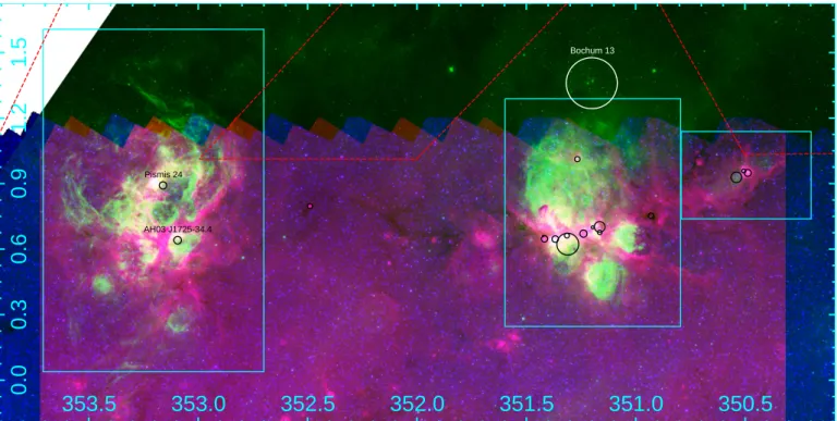
Pismis 24 AH03 J1725-34.4 Bochum 13Fig. 1. General view (green, red and blue images are UKST Hα image and Spitzer IRAC band 4 and 1, respectively) of the GM1-24 (l ∼ 350.5◦),
NGC 6334 (l ∼ 351.2◦
), and NGC 6357 (l ∼ 353.2◦
) regions. Coordinates are Galactic coordinates. The main clusters are displayed, along with the embedded stellar clusters listed byMorales et al.(2013). The red dashed line displays the coverage of the VPHAS+DR2 survey (areas above the line where not yet observed in the DR2 release). The delimitation area of the regions NGC 6357, NGC 6334 and GM 24 are shown as cyan rectangles. We also note that the Spitzer IRAC survey does not cover galactic latitudes larger than 1.1◦
.
both regions mainly based on the Gaia DR2 data. The
kinemat-ics of the ionized (Russeil et al. 2016) and molecular gas (André
et al. 2016;Zernickel et al. 2013) have been extensively studied
before. In this study, we use Gaia DR2 (Gaia Collaboration 2018)
proper-motion data to determine if any of the systematic motions of the YSO and OB stellar populations can be used to better understand the star-formation history of these regions. Already,
for NGC 6357,Gvaramadze et al.(2011) identified, based on
pre-vious astrometric measurements, runaway stars (and their bow-shock features), which are important for probing the dynamics of the native condition for massive stars. In the following, we
delin-eate the studied regions as shown in Fig.1. The spatial limits of
the each region is mainly based on the Hα (ionized gas) extension.
NGC 6357 coverage is 352.7◦≤ l ≤ 353.7◦and 0.27◦≤ b ≤ 1.6◦,
for NGC 6334 it is 350.8◦ ≤ l ≤ 351.6◦ and 0.24◦ ≤ b ≤ 1.3◦,
and for GM1-24 (a H
ii
region centered at l, b ∼ 350.5◦, 0.96◦),it is 350.2◦≤ l< 350.8◦and 0.74◦≤ b ≤ 1.14◦.
This paper is organized as follows. In Sect. 2, we present
the Gaia DR2 data, the selection criteria used, and the
calcu-lated quantities. In Sects. 3and4, we present our OB star and
YSO samples and we discuss the results in Sect.5. Section6is
devoted to the conclusion.
2. Gaia DR2 data description
The Gaia DR2 catalogue (Gaia Collaboration 2016,2018)
pro-vides astrometric data, with errors, for positions (α, δ), proper
motions, µα, µδ, and parallaxes, π, in addition to photometric
data (G, Rp, and Bpmagnitudes).
The samples discussed in this paper come from optical data
(ESO-VLT VIMOS and VPHAS+ DR2) and the infrared Spitzer
IRAC/GLIMPSE survey. The typical seeing was 1.100 and 0.900
and the pixel size was 0.20500 and 0.2100 for the ESO-VLT
VIMOS and VPHAS+ DR2, respectively, while for Spitzer
IRAC/GLIMPSE the typical point spread function is 1.800(Fazio
et al. 2004) and pixel size is 0.600. In parallel, to evaluate the
effect of proper motions on the cross-match with Gaia DR2 data,
we retrieved the Gaia DR2 sources within a typical cone with a
radius of 100(size chosen to ensure a statistically representative
sample) centered on NGC 6334 and NGC 6357 and we trans-form Gaia J2015.5 coordinates into J2000 (using the dedicated TOPCAT tool). We find a mean separation between J2015.5 and
J2000 coordinates of 0.055300 and 0.055800 for NGC 6334 and
NGC 6357, respectively, with a maximum separation of 0.8500.
This suggests a tolerance radius of 0.700for the optical data and
1.300 for Spitzer IRAC/GLIMPSE. We also retrieved the Gaia
DR2 sources within a cone with radius of 300(size allowing to
probe correctly a representative surface density of the sources) centered on NGC 6334 and NGC 6357 from which we
evalu-ate a mean distance between the sources of 0.800 and 1.400 for
a 100and 200 cone search, respectively. In addition, we estimate
that 1.3% of the Gaia sources have at least one neighbor within
100against 7% within a 200cone search. Thus, a tolerance radius
of 100 seems to be a good compromise between the input data
astrometric precision and the typical Gaia sources density in our field. This leads us to do the best cross-matching with the Gaia
DR2 catalog, adopting a tolerance radius of 100.
Lindegren et al. (2018) reported a systematic shift in the
GaiaDR2 parallaxes corresponding to a zero-point correction
of −0.03 mas. However, studies of different types of Galactic
objects give zero-point offsets between −0.031 and −0.08 (e.g., Graczyk et al. 2019; Stassun & Torres 2018). For example, Navarete et al.(2019) point out the impact of the parallax zero-point correction to the distance of W3 complex, showing a distance decrease of up to 15% (with the larger zero-point cor-rection). In this context, we performed no corrections of parallax
zero-point in this paper. The proper motions were also converted
from equatorial to galactic coordinate system (µl, µb), following
Vogel(2013).
To properly study the tangential velocity of stars, we have to correct the observed proper motions from the peculiar solar motion and its systematic motion due to the Galactic rotation.
This correction was done following Abad & Vieira (2005)
and Mignard (2000) adopting the Oort’s constants A=
15.1 km s kpc−1 and B= −13.4 km s kpc−1 (Li et al. 2019) and
the components for the solar peculiar velocity (U , V , W )=
(11.1,12.24,7.25) km s−1 respectively to the Local Standard of
Rest (Schönrich et al. 2010). The corrected proper motions
will be noted as µlcor, µbcor, from which we calculate Vlon and
Vlat (the components of the velocity in the regions Galactic frame). These velocities represent the residual velocities which characterize the non-circular motion in the Galactic disk and also the velocity respectively to the interstellar medium.
With regard to the distance, Bailer-Jones (2015) and
Astraatmadja & Bailer-Jones(2016a,b) recall that a star’s reli-able distances cannot be obtained by simply inverting the par-allax when the relative parpar-allax error is larger than 0.2 and for negative parallaxes. In this way, we also retrieved “the best esti-mate of distance using the exponentially decreasing space
den-sity prior” with the standard value L= 1.35 kpc as a scale-length
parameter (as recommended byBailer-Jones 2015;Astraatmadja
& Bailer-Jones 2016a) and the 5th and 95th percentile confi-dence intervals using the TOPCAT tool. This is a probality-based
inference approach (Bayesian method) described by
Bailer-Jones (2015), Astraatmadja & Bailer-Jones (2016a), and Luri et al.(2018). This distance is noted as dbay.
Finally, the renormalized unit weight error (RUWE) is also considered. A RUWE value larger than 1.4 could indicate that the source is non-single or otherwise problematic for the astro-metric solution (Gaia technical note
Gaia-C3-TN-LU-LL-124-01). Thus, in the following (aside from Sect.3.1), we apply the
selection criteria: π > 0, RUWE ≤ 1.4, and σπ/π ≤ 0.2.
3. OB star samples
3.1. Sample of spectroscopic OB stars
The spectroscopic catalog consists of the sample of 135 O-B3
stars fromRusseil et al.(2017). This sample, listed in TableB.1,
is composed of 109 spectroscopic O-B3 stars (identified by a
number in Table B.1) supplemented with 26 O-B3 stars
(iden-tified by their name1 in Table B.1) from the literature (listed
and referenced in Table A.2 of Russeil et al. 2017) for which
we have spectral types, V-band magnitudes, and extinctions, as well as spectro-photometric distance. After cross-matching with
Gaia DR2, we compared the Gaia-G and V-band magnitudes
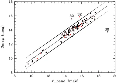
(see Fig.2). Three stars (stars 30, 32 and 82) clearly depart from
the trend by more than 2σ (Fig.2). In order to pinpoint the
possi-ble origin of this departure, we cross-matched our OB star
sam-ple with the VPHAS-DR2 catalog (Drew et al. 2014).
For stars 82 and 32, the V-band and VPHAS-DR2-g agree well, suggesting that their Gaia-G brightness may not be well determined. Indeed, star 32 has a RUWE larger than 1.4 suggest-ing binarity and also its parallax error is larger than 20%. Star 82 has no parallax measurement. Thus, we decided to remove these two stars from the rest of the analysis.
Star 30 shows agreement between VPHAS-DR2-g and Gaia-G, suggesting an erroneous value for the V-mag. It is likely
1 This name comes from the SIMBAD astronomical database:
http://simbad.u-strasbg.fr/simbad/
Fig. 2.Gaia-G versus V-band magnitude. The linear regression fit (cen-tral line) gives the relation G= 0.831(±0.026)×V +1.528(±0.382). The two lines on both sides of the linear regression fit delineate the 2σ band. Black (red) symbols indicate OB stars filling (not filling) the full selec-tion criteria (π > 0, RUWE ≤ 1.4, and σπ/π ≤ 0.2).
Fig. 3. Parallax versus longitude plot of spectroscopic OB stars. Green, blue, red, and black points are stars belonging (in the area delineated in Fig.1) to GM1-24, NGC 6334, NGC 6357, and also to none of them, respectively.
that the reason for this uncertainty is contamination by a nearby
star. Indeed, we found in the Russeil et al. (2017) catalog, a
star at less than 1.200with a brightness in better agreement with
Gaia-G. For this star, we then updated the V-band magni-tude and, hence, its spectrophotometric distance (changing from 6.94 kpc to 2.47 kpc), placing it in better agreement with the dis-tance of the region.
Since we selected stars with π > 0, RUWE ≤ 1.4, and σπ/π ≤
0.2 in the following, we have a final sample of 88 spectroscopic
OB stars expected to be barely affected by binaries. This
selec-tion criteria is applied to all following samples.
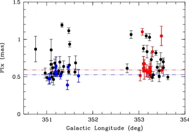
In Fig.3, the final spectroscopic OB stars sample is presented
in a parallax versus longitude plot. The mean astrometric
param-eters are given in Table1.
3.2. Sample of photometric OB stars
To complete the spectroscopic OB stars sample, we used the
Table 1. Mean(1) parameter values for the spectroscopic OB stars sample. All NGC 6357 NGC 6334 Sample N 88 24 30 π (mas) 0.576 ± 0.076 0.586 ± 0.095 0.561 ± 0.075 dbay(kpc) 1.80 ± 0.31 1.76 ± 0.30 1.88 ± 0.42 µα(mas yr−1) −0.308 ± 0.846 −0.854 ± 0.770 0.106 ± 0.561 µδ(mas yr−1) −2.171 ± 0.767 −2.508 ± 0.666 −1.863 ± 0.599 µl(mas yr−1) −2.020 ± 0.845 −2.536 ± 0.616 −1.472 ± 0.393 µb(mas yr−1) −0.981 ± 0.576 −0.562 ± 0.303 −1.240 ± 0.728 µl cor(mas yr−1) −0.654 ± 0.832 −1.157 ± 0.684 −0.167 ± 0.575 µb cor(mas yr−1) 0.024 ± 0.656 0.543 ± 0.378 −0.116 ± 0.859 Vlon (km s−1) −5.043 ± 8.571 −10.487 ± 11.738 −1.426 ± 6.551 Vlat (km s−1) −0.211 ± 5.399 3.920 ± 2.521 −2.074 ± 6.345 PA(2)(◦) 224 ± 91 284 ± 55 183 ± 97
Notes.(1) Except for PA and d
baythese are 3 σ clipping mean values.
All the uncertainties are computed as the standard deviation.(2) PA, is
the position angle counted from the Galactic north direction toward the increasing longitude axis direction.
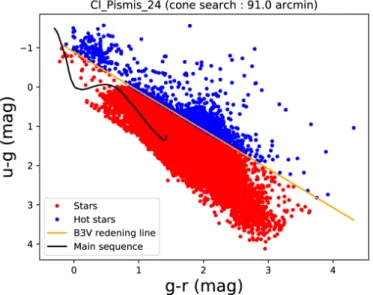
Fig. 4. u −g versus g − r plot for stars towards NGC 6357 (within 910
centered on the Pismis 24 cluster). The B3V star reddening vector and the main sequence are fromDrew et al.(2014). Hot stars are those that are earlier than B3V.
sources with u, g and r magnitudes in the area covering l= 350◦–
354◦and b= −0.5◦–+2◦. However, from Fig.1, we notice that
only a few small areas in our region of interest are not covered
by the VPHAS+ DR2 survey. The VPHAS+ DR2 basic
carac-teristics are: a median seeing bewteen 0.800 and 1.0100, a typical
depth of 20 mag in u, g and r and saturation problems, occur-ring for stars brighter than 13. In addition, due to the uncertainty
around the initial calibration, a field-dependent offset has been
noted (Drew et al. 2014;Mohr-Smith et al. 2017). This leads to
larger uncertainties for the u-band magnitudes. These typical o
ff-sets are ∼–0.35, ∼0.05, and ∼0.01 for the u, g, and r magnitudes,
respectively (Mohr-Smith et al. 2017).
Similarly toMohr-Smith et al.(2017) andChen et al.(2019),
we plot the stars in the u − g versus g − r plot and select stars above the B3V star reddening law. For this first selection step,
we adopted the curve of the B3V stars fromDrew et al.(2014).
Figure 4 illustrates this process for stars in the direction of
NGC 6357 (centered on the Pismis 24 cluster). We then
cross-Fig. 5.Parallax versus longitude plot of photometric OB star sample. Green, blue, red and black points are stars belonging (in the area delin-eated in Fig.1) to GM1-24, NGC 6334, NGC 6357 and to none of them respectively.
correlated this sample with Gaia DR2 and found 2233 OB stars that have Gaia information. Stars above this reddening law are
expected to be normal OB stars butChen et al.(2019) show that
because of the large uncertainties in the u-band magnitudes, they are strongly contaminated by B4 and later type stars, sub-dwarfs,
and white dwarfs. FollowingChen et al.(2019) we then plot stars
in the Gaia color-absolute magnitude diagram and apply a sec-ond selection step by keeping only stars above the B3V
extinc-tion vector (earlier than B3V) ofMaíz Apellániz et al.(2014).
The final reliable photometric OB stars sample contains 174
objects (following π > 0, RUWE ≤ 1.4, and σπ/π ≤ 0.2) which
are mostly located towards NGC 6357 and NGC 6334. To esti-mate the reliability of the photometric catalog, we compared it with the spectroscopic catalogue. We find that 51 spectroscopic OB stars can be paired with a photometric OB star. Among the 84 not paired spectroscopic OB stars, 38 have no u, g, or r mag-nitudes, which naturally explains why they are not found in the photometric catalog (these stars are mainly bright stars, with
V < 13 mag, and then they are in the VPHAS+ DR2
satura-tion domain), while the remaining 46 stars are all B1 to B3 stars and were missed during the first step selection because they fall below the reddening law due to the u-band photometric uncer-tainty.
In Fig.5, the photometric OB stars sample is presented in a
parallax versus longitude plot. The mean astrometric parameters
are given Table2.
4. YSOs samples
YSOs are recently formed stars that are typically found in or very near their parental molecular cloud. During the early-phase
of their formation (class 0/I), they are strongly embedded in their
accreting envelope, which makes them not easy to observe at the optical wavelengths. During their evolution, they become pre-main sequence stars with prominent circumstellar disks (class II) whose emission peak moves from the infrared to the visible
as the disks dissipate.Marton et al.(2019) found that 55% of the
YSOs detected by Spitzer are present in the Gaia DR2 catalog
and 68% of them are brigther than Gmag= 17. In the Orion A
molecular cloud,Großschedl et al.(2018) found 67% of YSOs
with a Gaia DR2 counterpart are mainly Class II sources. How-ever, these fractions are for nearby regions and at the distances
Table 2. Mean parameter values for the photometric OB stars sample. All NGC 6357 NGC 6334 Sample N 157 80 55 π (mas) 0.554 ± 0.070 0.561 ± 0.084 0.552 ± 0.054 dbay(kpc) 1.75 ± 0.24 1.74 ± 0.28 1.75 ± 0.17 µα(mas yr−1) −0.429 ± 0.675 −0.874 ± 0.398 0.092 ± 0.468 µδ(mas yr−1) −2.055 ± 0.621 −2.332 ± 0.522 −1.746 ± 0.532 µl(mas yr−1) −1.950 ± 0.752 −2.460 ± 0.495 −1.412 ± 0.438 µb(mas yr−1) −0.808 ± 0.558 −0.569 ± 0.487 −1.054 ± 0.479 µlcor(mas yr−1) −0.719 ± 0.851 −1.293 ± 0.564 −0.145 ± 0.518 µbcor(mas yr−1) 0.211 ± 0.568 0.440 ± 0.505 −0.022 ± 0.467 Vlon (km s−1) −6.362 ± 7.790 −11.071 ± 7.165 −1.657 ± 4.214 Vlat (km s−1) 1.575 ± 4.740 3.406 ± 4.260 0.065 ± 4.384 PA (◦) 235 ± 92 281 ± 51 179 ± 106
Notes. Except for PA and dbay, these are 3 σ clipping mean values
val-ues. All the uncertainties are computed as the standard deviation.
of NGC 6334 and NGC 6357, we expect them to be smaller. A direct distance and proper motion determination of YSOs thanks to Gaia DR2 is a new way to determine the distance of their native molecular cloud and to probe their kinematics. This has
been done, for instance, byGroßschedl et al.(2018), who
actu-ally delineated the 3D shape of the Orion A molecular cloud and by Fleming et al. (2019), who identified two groups of YSOs belonging to the Taurus molecular cloud and moving in
some-what different directions.
4.1. Previously published YSO catalogs
We consider the infrared-excess source catalog (covering
NGC 6334 and NGC 6357) fromPovich et al.(2013). This
cat-alogue was constructed by Kuhn et al.(2014), as part of the
MYStIX project (Feigelson et al. 2013) which surveyed 20
OB-dominated young clusters using a combination of Spitzer
IRAC (Fazio et al. 2004) infrared and Chandra (Weisskopf
2000) X-ray photometry. For NGC 6334 and NGC 6357 the
sur-veyed area is 1◦ diameter. Identification and classification of
YSOs were carried out byPovich et al.(2013) who used Spitzer
IRAC, 2MASS (Skrutskie et al. 2006), and UKIRT (Lawrence
et al. 2007) imaging photometry with spectral energy
distribu-tion fitting to flag sources as “‘0/I”, “II/III”, “non-YSO
(stel-lar)” or “Ambiguous (YSO)”. In addition, they estimated the
membership probabilities (Mm= 1 for probable members
other-wise Mm= 0) from the spatial distribution. We cross-matched
the Povich et al.(2013) catalog with Gaia DR2 and selected
only member sources (Mm= 1) flagged “0/I” and “II/III”. We
obtained a sample of 27 YSOs (10 in NGC 6334 and 17 in
NGC 6357). In NGC 6334 all the YSOs are class II/III, while
4 among 17 are class 0/I in NGC 6357. Because class 0/I YSOs
are more embedded than class II/III, and because Gaia is an
opti-cal telescope and has difficulty accurately measuring parallaxes
in areas of high optical extinction, as is the case in star-forming regions, we expect to find fewer counterparts with Gaia DR2
for class 0/I than for class II/III YSOs. This YSO sample is
presented as a parallax versus longitude plot in Fig.6 and the
mean astrometric parameters are given in Table 3. The
paral-lax and proper motion (see Sect. 5.3) of several non-member
sources (Mm= 0) imply that they should be assigned to the
regions that redefine the YSO samples (named NGC 6334-sub
and NGC 6357-sub in Table3).
We considered also the YSO catalog (2281 sources) from Willis et al.(2013) covering only NGC 6334. We find only 302
YSOs in common between Willis et al. (2013) and the 688
Fig. 6. Parallax versus longitude plot of YSOs from Povich et al.
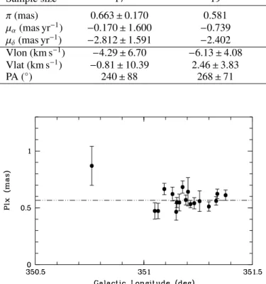
(2013). The color coding is the same as in Fig.3. The blue and red lines display the mean parallaxes for NGC 6334 and NGC 6357, respec-tively (excluding outliers). Black symbols are sources classified as non-members byPovich et al.(2013).
sources in NGC 6334 from Povich et al. (2013). Willis et al.
(2013) find more YSOs in the NGC 6334 ridge and the di
ffer-ence between these two samples certainly resides in the selec-tion process. However, among the 2281 listed YSOs, only 19 follow our full selection criteria. They are presented in the
paral-lax versus longitude plot of Fig.7. Among them, there is one star
with a very large parallax (π = 4.46 mas, not shown on Fig.7)
and 17 appear to be located along the main NGC 6334 molecu-lar ridge. The mean astrometric parameters for this sample are
given in Table 3. We wanted to consider the YSOs fromFang
et al.(2012), covering only NGC 6357, but their YSO catalog is not publicly available.
4.2. Larger scale study of YSOs
Because the catalog of Povich et al. (2013) only probes
the central regions in NGC 6334 and NGC 6357, we use the
IRAC/GLIMPSE point source catalog to do a larger scale census
of the YSOs towards NGC 6334 and NGC 6357.
The most frequently used classification scheme for YSOs is
the class 0/I-II system, which characterizes the objects in terms
of their IR excesses or SEDs (e.g.,Adams et al. 1987;André
et al. 1993,2000). Class 0 and I objects are understood to be protostars surrounded by dusty infalling envelopes while Class II objects are pre-main-sequence stars with warm optically thick dusty disks orbiting around them. To classify an IRAC source
we follow Billot et al.(2010) who show that sources with the
following color constraints are considered likely to be YSOs: [4.5]−[8.0] > 0.5
[3.6]−[5.8] > 0.35
[3.6]−[5.8] ≤ 3.5 × ([4.5]−[8.0])−1.25.
We further classify the selected objects according to their
infrared spectral index αIR = d(log(λFλ))/d log(λ) as defined
by Lada et al. (1987). We compute the spectral index as the slope of the spectral energy distribution (SED) measured from
3.6 to 8.0 µm. Objects with αIR > −0.3 are designated class I
Table 3. Mean motion parameters values for YSOs.
NGC 6357 NGC 6357-sub NGC 6334 NGC 6334-sub NGC 6334-ridge
Povich et al.(2013) Povich et al.(2013) Povich et al.(2013) Povich et al.(2013) Willis et al.(2013)
Sample size 17 19 10 19 17 π (mas) 0.663 ± 0.170 0.581 0.528 ± 0.075 0.565 ± 0.074 0.566 ± 0.066 µα(mas yr−1) −0.170 ± 1.600 −0.739 −0.313 ± 0.796 0.120 ± 0.341 0.086 ± 0.419 µδ(mas yr−1) −2.812 ± 1.591 −2.402 −1.789 ± 1.482 −1.830 ± 0.341 −1.733 ± 0.376 Vlon (km s−1) −4.29 ± 6.70 −6.13 ± 4.08 −1.37 ± 11.18 1.80 ± 2.42 2.35 ±3.85 Vlat (km s−1) −0.81 ± 10.39 2.46 ± 3.83 1.39 ± 9.15 −0.800 ± 3.09 0.05 ± 3.31 PA (◦) 240 ± 88 268 ± 71 159 ± 98 134 ± 84 125 ± 77
Fig. 7. Parallax versus longitude plot of YSOs fromWillis et al.(2013).
a cold dusty envelop infalling onto a central protostar. Objects
with −0.3 ≥ αIR > −1.6 are classified as class II YSOs.
Because it is difficult to take into account the actual
extinc-tion of each source due to local features such as the associ-ated core and disk, we compute the spectral index with a global
extinction correction of AV = 6 mag, corresponding to the
mean foreground extinction in the direction of NGC 6334 and
NGC 6357 (Russeil et al. 2016). Indeed, the extinction, which
impacts the shorter wavelengths more than the longer ones, can
induce an artificial higher αIRvalue.
The global spatial distribution of class I and II selected YSOs
(3768 sources) is shown in Fig. 8a. Compared with Povich
et al. (2013) and Fang et al. (2012) for the central region of
NGC 6357 and withPovich et al.(2013) andWillis et al.(2013)
for NGC 6334, we find that our Spizer-IRAC- selected YSOs distribution is in agreement with their results.
For NGC 6334, considering the same area, there are 2228,
644 and 900 YSOs found byWillis et al.(2013),Povich et al.
(2013), and this work, respectively. As already noted, Willis
et al.(2013) found more sources in the ridge thanPovich et al.
(2013) and than we have. We have 328 (36%) and 466 (52%)
sources in common with Povich et al.(2013) andWillis et al.
(2013), respectively, most of them located along the ridge. For
NGC 6357, we find the same YSO overdensities asPovich et al.
(2013) andFang et al.(2012). which are the clusters Pismis 24
and AH03J1525-34.4, as well as the overdensity around l, b =
353.08◦,+0.63◦. Considering the same area, 670 and 768 YSOs
are found by Povich et al. (2013) and our study, respectively,
with 347 (45%) of our candidates paired and most of them being in the overdensities.
Fang et al. (2012), Willis et al. (2013), and Povich et al.
(2013) complemented their IRAC sources classification with J,
Hand Ksobservations, which allowed them to detect lower mass
and lower luminosity YSO candidates than us and to access sources in bright nebulous regions that are saturated in the IRAC
observations. In addition. becauseWillis et al.(2013) use 24 µm
data they are able to detect more embedded sources.
How-ever, sincePovich et al.(2013) used SED fitting to classify the
sources, their evolutionary classification is expected to be bet-ter defined. In particular, they have a betbet-ter debet-termination of the extinction, while our basic extinction correction leads us to over-estimate the number of YSOs.
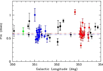
Cross-matching our YSOs sample with Gaia DR2 leaves us with 66 YSOs mainly located in NGC 6334 and NGC 6357 and
presented in Fig.9 as a parallax-longitude plot. Because of the
scarce number of confirmations, we mainly used our larger scale
YSO sample to identify possible new clusterings (see Sect.5.5).
5. Data analysis
5.1. Extinction
In this section, we present an analysis of the AG extinction2
dependency with the distance in order to make a first order deter-mination of the distance to the molecular cloud complex where our regions of interest are located. Indeed, the variation of the optical extinction with respect to the distance provides
informa-tion about the distance of the different extinction layers present
along the line of sight. This well-known method (e.g.,Magnani
et al. 1985;Schlafly et al. 2014) was recently used for Gaia DR2
data byYan et al.(2019) to determine the distance of high
lati-tude molecular clouds. However,Andrae et al.(2018) recall that
AG has large uncertainties and that extinction is then only
reli-able on average.
To produce the AG– distance plots, we extracted the Gaia
DR2 data within a 1◦ radius area centered on the four
fol-lowing positions: (1) NGC 6334, (2) NGC 6357, (3) at l,b =
352.2◦,+0◦ a position towards the Galactic plane and in
lon-gitude midway (to minimize contamination from both regions) between NGC 6334 and NGC 6357, and (4) in a reference
direc-tion (off cloud) pointing at l, b = 352.2◦, +3◦ a relatively
high latitude position (see AppendixA). We selected stars with
π > 0, σπ/π ≤ 0.2, and AG > 0. We then calculated the
error-weighted average and standard deviation of AGin 0.05 mas
par-allax bins and plotted the extinction versus distance in Fig.10.
In Fig.10a, we note that around 2 kpc AGdecreases instead of
increasing. This is caused by the combination of the magnitude limit (G ≤ 17) and the dwarf-giant bimodality in the stellar
2 We can recall that A
Fig. 8. YSO distribution and cluster identification. Figures are: (a) the YSO spatial distribution (black dots), (b) the 2D YSO clustering identi-fication (colored dots), and (c) the clustered stars from Gaia information (in red) overplotted on the 2D YSO groups (black dots). Each group is labeled as in Table4. NGC 6357 (dashed double dotted line), NGC 6334 (short dashed line), and GM1-24 (solid line) regions are delineated on every panel.
distribution. These effects are illustrated by Fig. 18 inAndrae
et al. (2018) and Fig. 8.20 in the Gaia data release
documen-tation3. In particular Andrae et al. (2018) show that the A
G
is limited to 3.5 mag for low temperature stars and falls down
to ∼1 mag for hot stars. That color effect strongly impacts the
3 See documentation release 1.2 at the link: https://gea.esac.
esa.int/archive/documentation/GDR2/
Fig. 9. Parallax versus lontgitude plot of Spitzer IRAC/GLIMPSE selected YSOs (b > 0.2◦
). The color coding is the same as Fig.3. The blue and red lines display the mean parallax value for NGC 6334 and NGC 6357, respectively.
Fig. 10. Extinction curves (a) towards NGC 6334 (blue), NGC 6357 (red), Galactic plane direction (black) and off cloud direction (black crosses) and∆AG = AG(region) – AG(off cloud) curves (b).
extinction curve, explaining the systematic curve decreasing after a certain distance around ∼1 kpc. In practice, this means that this method is not reliable for regions farther than ∼2 kpc and then, it is scarcely valid here for NGC 6334 and NGC 6357 which are located around 1.7 kpc. To remove these systematic
effects (see AppendixA), we produce the extinction curve
rel-atively to an off cloud position (Fig. 10b). In addition, due
to the position of the regions, close to the galacic plane, we can expect that the line of sight will cross several and very
inhomogeneous extinction layers, making the analysis difficult.
From Fig. 10a we notice that the extinction is higher towards
NGC 6357 than towards NGC 6334, while from Fig.10b, which
plot∆AG= AG(region) – AG(off cloud) versus distance, we note
a strong extinction feature around 1.3 kpc with possibly a sec-ond, smaller extinction bump around 1.7 kpc and around 3 kpc, an other possible extinction layer.
These results are in agreement with Russeil et al. (2016),
who also found higher extinction toward NGC 6357 (AV ∼
6.6 mag) than toward NGC 6334 (AV ∼ 5.1 mag). Our extinction
features are consistent with the OB star distribution peaks around
1 kpc, 1.8 kpc, and 2.6 kpc found byRusseil et al.(2012), where
the two first stellar peaks are assigned to the Sagittarius-Carina arm and the third one to the Scutum-Crux arm. It is not the first time that observations suggest that the Sagittarius-Carina arm
is split into two stellar layers (e.g.,Carraro 2011;Russeil et al.
2017;Mel’Nik et al. 1998), where the closer layer (which cor-responds to the outer edge of the arm with respect to the galac-tic rotation) is populated by older stars while the farther layer (corresponding to the inner part of the arm) is more populated
by young stars. In addition, Mel’Nik et al. (1998) observed a
change in the residual velocities of the associations from the inner to the outer edges of the Carina arm, accompanied by a stellar age stratification, which they find is in agreement with what is expected for spiral density waves within the corotation
radius. More recently,Lallement et al. (2019), built a 3D map
of the dust distribution within 2 kpc around the Sun, revealing a particularly compact and well-delineated foreground region of the Sagittarius-Carina arm that extends in the fourth quadrant
and at 0◦< l < 30◦in the first quadrant. Appearing as a series of
compact cloud complexes that are well-aligned in the l = 45◦–
225◦ direction, they note that the clouds of this region, at the
fourth quadrant, may be as close as 1 kpc. They put in evidence of a second and similarly compact outer region (but oriented in the direction of rotation) of Sagittarius–Carina arm located at larger distance (∼2 kpc) and predominantly 50–150 pc above the Galactic plane. They interpret this split of the Sagittarius-Carina arm as a complex wavy structure. With a typical height
of 25 pc above the Galactic plane(assuming d = 1.75 kpc and
b ∼0.8◦for both regions), NGC 6334 and NGC 6357 are located
halfway between these two structures. 5.2. Distance
The distance to NGC 6334 and NGC 6357 has been discussed in several previous works. From the spectrophotometric study of the O-B3 star sample, a distance of 1.75 kpc was adopted (Russeil et al. 2017). The studies of individual clusters (e.g., Massey et al. 2001;Kharchenko et al. 2013,2016) report dis-tances within 1.5 kpc and 2.5 kpc. The maser parallax of the
source NGC 6334I(N) gives a distance of 1.35 kpc (Chibueze
et al. 2014; Wu et al. 2014). Recently, in the direction of NGC 6357 and NGC 6334, two open clusters, Pismis 24
(l, b= 353.16◦,+0.89◦) and Bochum 13 (l, b= 351.21◦,+1.38◦),
were studied from Gaia DR2 data byCantat-Gaudin & Anders
(2020). They determined dbay= 1677.5 pc and 1679.4 pc
respec-tively while the cluster Bochum 13 was up to now placed at a
distance of 1.34 kpc (Kharchenko et al. 2013).
Figure 11 shows that the direct comparison of
spectro-photometric stellar distance with the Gaia dbay is not obvious.
Fig. 11. Gaiaversus spectro-photometric distances. Red points are giant stars. The line displays the one to one correspondance.
Grosbøl & Carraro(2018) noted a similar discrepancy between parallactic and spectroscopic distance of a sample of B and A-type stars, suggesting that multiple-star systems and giants stars can explain shorter and larger spectroscopic distance than
Gaiadistance, respectively. We roughly find also that most of the
giant stars have larger spectro-photometric distance than Gaia distance. This underlines the fact that considering individual stellar Gaia distance is not reliable and that we must always con-sider them statistically.
Because it is the best-defined sample and because OB stars are more appropriate for statistically determining the distance of the regions, to add constraints on the distance we mainly use the parallax information from the spectroscopic OB star
sam-ple (see Fig.3). For these regions, we find a 3σ clipping mean
parallax of 0.575 ± 0.076 (d= 1.74 kpc), a mean parallax of
0.572 ± 0.083 mas (d= 1.75 kpc), a mean dbayof 1.80 ± 0.32 kpc,
and an error weighted average of 0.568 ± 0.005 mas (Table 1)
corresponding to a distance of 1.76 kpc. These values all agree and confirm the usual adopted distance. We can then define a parallax range for a star to belong to NGC 6334– NGC 6357 layer as: 0.48 < π < 0.67 mas. From the OB star sam-ples, we note few stars with π ∼0.8 mas (these stars are not located at particularly high latitude). This foreground popula-tion may be associated with the Sco-OB4 associapopula-tion located
at l, b = 352.64◦,+3.23◦ (Mel’nik & Dambis 2017) for which
Kharchenko et al.(2013) andMel’nik & Dambis(2017) give a
mean distance (and mean proper motion) of 1.1 kpc (µα, µδ =
0.50 ± 0.19 mas yr−1, −2.90 ± 0.19 mas yr−1) and 0.96 kpc (µ
l,
µb= −1.34±0.42 mas yr−1, −2.70 ± 0.29 mas yr−1), respectively.
Indeed, Roslund (1966) found that the Sco-OB4 association
extends towards the south with a concentration of high luminosty
stars in the H
ii
regions of NGC 6334 (and suggest that theseexciting stars form an association). In this extension, between
Sco-OB4 and NGC 6334, there are stars (e.g., Fig. 8 ofRoslund
1966) which can now be assigned to the cluster Bochum 13. We
can then suspect that our samples might be contaminated by Sco-OB4 stars or that NGC 6334 OB stars could be part of this
asso-ciation. Indeed, studies of the Scorpius-Centauraus (Wright &
Mamajek 2018) and Vela-Puppis (Cantat-Gaudin et al. 2019a) stellar complexes have revealed that even very young stellar pop-ulations can exhibit sub-structured and non-centrally concen-trated spatial distributions (spanning hundreds of parsecs) and
that their overall distribution can reflect the primordial gas distri-bution, rather than the disruption of an initially compact cluster.
Using the YSO parallaxes (Figs.6,7,9), we can see that
most of the YSOs belong to NGC 6334–NGC 6357 and that just a few of them display also a larger parallax (π between 0.8 mas and 1.1 mas). This may suggest that a foreground population of
young stars could exist between 0.9 and 1.25 kpc. Finally, Fig.6
suggests that several YSOs considered as non member inPovich
et al. (2013) have a parallax in agreement with NGC 6334 or NGC 6357 and, thus, they may belong to these regions.
5.3. Transverse motions
Because stars in clusters and associations share common kine-matic properties, in addition to the parallax, proper motions are used to distinguish any different group’s members from the back-ground stars. This method was used, for instance, to extract and
characterize stellar clusters and associations (e.g., Franciosini
et al. 2018;Cantat-Gaudin et al. 2018,2019b;Borissova et al. 2018;Zari et al. 2018), and even young stellar populations (e.g., Fleming et al. 2019). In parallel, any kinematic substructures can be assumed to be the remnant of the primordial phase-space structure during the formation stages, as has been
sug-gested for OB associations (e.g., Wright et al. 2016; Wright
& Mamajek 2018). Also, the stars, particularly the massive stars, are expected to be born in motion with respect to their surroundings because they keep the momentum that is gained during their star-formation process, where turbulence is needed,
with velocities of 2–5 km s−1 (e.g.,Peters et al. 2010; Dale &
Bonnell 2011). More recently,Kounkel & Covey(2019), identi-fied 1900 clusters and comoving groups within 1 kpc around the
Sun (and |b|< 30◦), showing that many of these groups present
filamentary or string-like morphologies that are oriented parallel to the Galactic plane and preferentially oriented perpendicular to the stellar streams. They suggest that the strings, which are most prominent in the youngest populations, are primordial and mirror the shape of the stellar parental molecular cloud. At this step, we note that none of their cataloged groups are in front of NGC 6334 and NGC 6357. The spatially closest group (Theia
290) is below the Galactic plane (l, b = 352.597◦,−0.850◦)
with π = 1.1827 mas (which can be converted to a distance of
∼845 pc).
Figures12and13show the sample distribution of OB stars
and YSOs in the proper motion and transverse velocities planes. In such plots, stars belonging to NGC 6334 and NGC 6357 show distinct mean proper motions. The mean values are summarized
in Tables1–3and the individual star transverse motion vectors
is presented in Fig.14.
Stars belonging to NGC 6357 and NGC 6334 show distinct motion while, spatially, stars in NGC 6357 are clearly clustered
(e.g., Kuhn et al. 2019) while in NGC 6334 they are sparser.
For NGC 6357 our average values agree with the mean ones of Cantat-Gaudin et al. (2018) for Pismis 24 (µα, µδ = −0.854 ±
0.218, −2.083 ± 0.320 mas yr−1, π = 0.567 ± 0.085 mas) and
with Kuhn et al. (2019), who distinguish three sub-structures
(Pismis 24, G353.1+0.6, and G353.2+0.7) with similar proper
motions and parallaxes (µα, µδ = −0.90 ± 0.08, −2.29 ±
0.10 mas yr−1, π= 0.56 ± 0.04 mas).
For NGC 6334,Dias et al.(2014),Kharchenko et al.(2013)
andSampedro et al.(2017) give very different values (−1.32 <
µα < −0.75 mas yr−1and −3.32 < µδ< 0.09 mas yr−1), however
their values were estimated from the UCAC4 (Zacharias et al.
2013) or PPMXL (Roeser et al. 2010) catalogs.Shi et al.(2019)
identify systematic errors in the position and proper-motion
sys-tems of the PPMXL and UCAC5 compared with the Gaia DR2. It is also important to notice that the works on NGC 6334 that we reference focus on a more contained area towards the region
H
ii
351.2+0.5, while our sample is more extended on the skyplane. However, the large spatial and kinematical dispersion of OB stars in NGC 6334 are more characteristic of an OB
associ-ation (e.g.,Mel’nik & Dambis 2017).
In NGC 6357, stars have a relatively ordered overall motion while in NGC 6334 stars show random direction of their motions
(Fig. 14). Globally NGC 6357 stars seem to move along the
Galactic planein the direction of NGC 6334 with a relative
veloc-ity of ∼9 km s−1 (and in the opposite direction of the galactic
circular rotation). Assuming that the OB stars still keep the kine-matic signature from their birth places, this sets constraints on the star formation origin. The fact that OB stars in NGC 6357
and NGC 6334 show different motions and spatial distribution
suggest that they were formed independently from each other
and under different conditions, with OB stars in NGC 6334
resembling more an OB association while they form clusters in NGC 6357.
For regions farther than 1 kpc, Cantat-Gaudin & Anders
(2020) show that group proper motion dispersions (measured
from Gaia DR2 data) are dominated by measurement
uncer-tainties with a typical value around 0.2 mas yr−1, while groups
with large proper motion dispersion are either non-physical
clus-ter or substructured aggregates (see Fig. 1 in Cantat-Gaudin
& Anders 2020). Here the mean proper motion dispersion for
OB stars of 0.86 mas yr−1and 0.74 mas yr−1for NGC 6357 and
NGC 6334, respectively, suggesting some substructuring. The
substructuring is confirmed for NGC 6357 byKuhn et al.(2019)
who used Gaia DR2 to study the kinematic properties of the
young stellar groups, Pismis 24, G353.1+0.6, and G353.2+0.7
located in NGC 6357. They show a possible expansion of Pismis
24 and G353.1+0.6 and they find that the subclusters motions
are divergent, rather than convergent (expected for assembling from smaller components), with relative motions randomly
ori-ented and with velocity between 2 and 5 km s−1(relative to the
center of mass of the entire group). This shows that the sub-clusters are not in the way of assembling and they suggest that their motions are more linked to the large-scale kinematics of the parental molecular cloud.
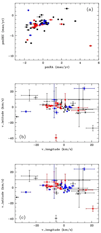
Despite the low number of sources, YSOs in NGC 6334 and NGC 6357 show, as the OB stars, respective distinct motions
(Table3). From Fig.13c, we can exclude the evident outliers
and define new sub-samples of sources (named NGC 6334-sub
and NGC 6357-sub in Table 3). In NGC 6357, YSOs are
spa-tially coincident with OB stars and follow similar motion. In NGC 6334, YSOs are mainly concentrated into the molecular
ridge (Willis et al. 2013) contrary to OB stars while their mean
motion is different from that of the OB stars.
5.4. Runaway candidates
Runaway stars are typically massive stars that move at large peculiar velocity with respect to the surrounding stars and inter-stellar medium. Observationally, if runaway stars are detected by their large proper motions or radial velocities with respect
to the surrounding stars (Tetzlaff et al. 2011), they can also be
evidenced from dusty bow shock features (observed on mid-IR images) formed ahead of their motion direction by the interaction between stellar winds and the surrounding medium where the relative velocity between the two is supersonic (e.g., Mac Low et al. 1991;Gvaramadze et al. 2011;Gvaramadze & Bomans 2008;Maíz Apellániz et al. 2018). However, bow-shock
Fig. 12.Proper-motion and transverse velocities plots of spectroscopic (panels a, b, and c) and photometric (panels d, e, and f) OB stars samples. In these plots, green, red, blue, or black symbols are stars belonging to GM1-24, NGC 6357, NGC 6334, and field stars, respectively. In panels (c) and (f), the box displays the limits from outside which a star can be considered as runaway (see Sect.5.4).
features can also be formed when a star is overrun by an ouflow
of hot gas coming from a H
ii
/star-forming region (Henney &Arthur 2019). In this case, the bow-shock is expected to face the
H
ii
region/star-forming region as it is observed in M16 (e.g.,Kobulnicky et al. 2016). They are classified as “in situ”
bow-shocks (Kobulnicky et al. 2016) and, thus, they are not related to
any runaway aspect.
Since runaway stars can be explained by different scenarios,
namely: (i) the binary supernova scenario (e.g., Blaauw 1961;
Renzo et al. 2019), which happens when the more massive pri-mary star in a close binary undergoes a core-collapse supernova;
(ii) the dynamical (and early) ejection in a cluster (e.g.,Poveda
et al. 1967;Allison et al. 2010;Banerjee et al. 2012); and (iii)
ejection during a cluster merger process (e.g.,Lucas et al. 2018),
we want to use the detected runaway stars in NGC 6357 and NGC 6334 to add some constraints on the stellar formation
con-ditions in these regions. Indeed, Lucas et al. (2018) underline
Fig. 13. Proper-motion (a) and transverse velocities (b) for YSO mem-ber stars fromPovich et al.(2013) (black symbols are sources classified as non members byPovich et al. 2013) and (c) from the new members selection. The color coding is the same as Fig.3.
to be dispersed in tidal tails, whereas for the dynamical ejection process, they should be ejected without any directional
prefer-ence. In parallel, Farias et al. (2019) show, in their modeling,
that even though the fraction of massive runaway stars appears
to be relatively constant with the star-formation efficiency, the
number of massive star ejections are larger in the fast forma-tion regime and that dynamical ejecforma-tions in slowly forming star clusters are more energetic but less numerous than in the fast
for-mation regime. During the forfor-mation of the clusters, the ejection rate remains high and is closely correlated to the number den-sities. As stars are formed, the central number densities grow, along with the ejection rates.
As was highlighted previously by several authors (e.g., Tetzlaff et al. 2011;Maíz Apellániz et al. 2018), the main imped-iment is having a robust selection criteria for finding runaway stars. The selection criteria for runaway stars in such earlier
studies were either based on spatial velocities (e.g., Blaauw
1961), tangential velocities (e.g.,Moffat et al. 1998), or radial
velocities (e.g.,Cruz-González et al. 1974) alone.Tetzlaff et al.
(2011) used a sample of 7663 young stars from the H
ipparcos
catalog to lead several approaches aimed at defining runaway stars. Plotting the distribution of the peculiar 3D space veloc-ity (absolute value of the velocveloc-ity) of the stars, they show the existence of a low-velocity group and a high-velocity group (containing the runaway stars), both fitted with a Maxwellian
function. Following Stone (1979), we assume that a star is a
probable member of the high-velocity group (thus, a runaway) if the velocity is larger than the intersection of the two curves
which is 28 km s−1. Because for lot of stars either the radial or
the tangential velocity is measured, to define the runaway
cri-teria, Tetzlaff et al. (2011) also determined the intersection of
the two curves for the 1D cases, as well as the tangential
veloc-ity. They obtained: |Vlat| > 11 km s−1, |Vlon| > 19 km s−1, and
|Vtot| > 20 km s−1respectively. In addition, since stars in clusters
and associations share a common motion,Tetzlaff et al.(2011)
add another criteria to define runaway stars as stars clearly point-ing away from the cluster mean motion. This allows them to identify low-velocity runaway stars.
Here, given that radial velocity is not available for most of the sources, we base our selection of runaway stars on the trans-verse velocity, which inevitably leads to us missing some of them. To select possible runaway stars in our OB stars sample, we combined the velocity criteria with the departure to the
com-mon motion by selecting stars with |Vlat| >11 km s−1or |Vlon| >
19 km s−1, respectively, to the mean transverse velocity values.
In the spectroscopic and photometric catalogs, we find 14 and 13 runaway candidates, respectively. Among them, there are 5 in common, adding up to a final sample of 22 runaway
can-didates (listed TableB.2), among which three were previously
identified byGvaramadze et al.(2011). For nine of them, their
runaway status is confirmed by the presence of a dust bow-shock
feature ahead their motion (Figs.B.1andB.2).
These candidates have parallaxes between 0.27 and 0.76 mas, and 15 and 7 of them, respectively, are found in the direction of NGC 6357 and NGC 6334. Keeping stars with 0.48 < π < 0.67 mas, we count 10 and 2 stars toward NGC 6357
and NGC 6334, respectively (see Fig.14). Based on these
sub-samples, we note that runaway candidates in NGC 6357
indi-cate a common motion away from a rough position around l, b=
353.3◦, 0.63◦, while the two stars identified towards NGC 6334
show no common origin. Still, we have to keep in mind that,
as underlined byBanerjee et al.(2012), for about 1% to 4% of
the OB stars ejected from a young cluster, their motion cannot be traced back to their parent clusters because of the two-step
ejection process (Pflamm-Altenburg & Kroupa 2010), in which
a massive binary is first ejected from its cluster and when the pri-mary explodes as a supernova, the secondary OB star continues on a diverted trajectory.
Since most of runaway candidates are found towards NGC 6357, we can suspect a link between stellar clustering and runaway stars while their spatial distribution, around NGC 6357
350:0 350:5 351:0 351:5 352:0 352:5 353:0 353:5 354:0 Galactic longitude (±) ¡0:2 0 0:2 0:4 0:6 0:8 1:0 1:2 1:4 1:6 G a la c ti c la ti tu d e ( ±)
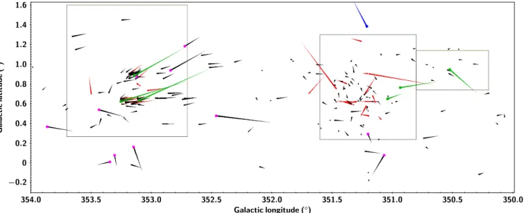
Fig. 14. Velocity vectors plots. Velocity vectors of OB stars (runaway OB star candidates are indicated by magenta dots) and YSOs are displayed as black and red arrows, respectively. Velocity vectors of YSO groups are displayed in green, while the Bochum 13 cluster (Cantat-Gaudin & Anders 2020) vector is displayed in blue. For clarity, taking the velocity vector length for Bochum 13 (4.79 km s−1) as reference, the YSO and
OB star vectors have been ploted with a relative scale of 0.33 and 0.11, respectively. Only stars and groups with 0.48 ≤ πle0.67 are shown. The squares delineate the regions: NGC 6357 (l ∼ 353.2◦
), NGC 6334 (l ∼ 351.2◦
), and GM1-24 (l ∼ 350.5◦
).
cluster. If such stars are related to the formation of clusters, the fact that many of them have not been observed towards NGC 6334 is surely because it is an OB association and this
suggests different formation conditions than for NGC 6357. As
underlined for the association Cyg OB2 byWright et al.(2014),
stellar ejection via dynamical encounters requires much higher stellar densities than are believed to have existed in Cyg OB2. 5.5. YSO larger scale study
Figure 8a shows some obvious agregates that underline
pos-sible YSOs clustering. To quantify this clustering we use the Python density-based spatial clustering (DBSCAN) algorithm
from the scikit-learn package (Ester et al. 1996;Schubert et al.
2017). This algorithm finds core samples of high density and
builds clusters from them. This algorithm was previously used byCastro-Ginard et al.(2018) to find clusters based on the Gaia
DR2 data. We divided the area of study (350◦ < l < 354◦) into
three sub-areas of∆l = 2◦which, as explained byCastro-Ginard
et al. (2018), allow the DBSCAN algorithm to define a more representative averaged density of stars required as a starting point. The definition of the DBSCAN cluster depends on two main parameters; one is the maximum distance (md) between two samples for one to be considered in the neighborhood of the other; the other parameter is the number of elements (minPts) in a neighborhood required for a position to be considered as a core
point. These parameters have been set to md between 0.05◦and
0.135◦(depending on the sub-area) and minPts= 20. Figure8b
shows the 15 resultant groups (with more than 30 stars) which
have been extracted and they are listed in Table4. Some of these
groups were already identified and classified as embedded
clus-ters or embedded groups byBica et al.(2019). Group 7 is clearly
related to GM1-24. In NGC 6357, our YSOs aggregates
corre-spond well to clusters found by Kuhn et al.(2014) andMassi
et al.(2015), as well as with the three YSOs overdense regions
identified byFang et al.(2012). In NGC 6334, we are not able
to find the clusters identified byKuhn et al.(2014) in the ridge.
This can be explained by incompletness due to the high intensity
level of the nebular emission in this part of the region, which
makes the point source detection difficult at IRAC bands. Our
sample is better at probing the YSO population near the edges of the ridge while a few additional aggregates are detected in the region between NGC 6334 and NGC 6357.
To better characterize these aggregates, we computed their
corresponding Minimum Spanning Tree (MST, e.g., Adami &
Mazure 1999). The MST algorithm builds a tree joining all the points of a given set by a segment, without a loop and with a min-imal length (each point being visited by the tree only one time). This tree is not unique, but the histogram of the segment’s length is unique. This allows us to characterize the set of points giving the mean, the dispersion (σ) and the skewness of the histogram
of the segments which are shown in the plots of Fig.15. The
MST analysis allows us to compare the YSO aggregates with typical distribution structures: core (King profile, used for
stel-lar cluster, e.g.,Bica & Bonatto 2011), cusp, filamentary
(estab-lished from extragalactic studies,Adami et al. 2010), and
ran-dom. In the s-σ plot (Fig.15), the backgrounds are close to the
filamentary distribution, suggesting that somewhat filamentary structure could be an intrinsic mode for the general YSOs distri-bution. We note that groups number 12 and 13 are well defined as core like clusters. It is not surprising as they correspond to the well-known clusters AH03J1525-34.4 and Pismis 24, respec-tively. Group 11, falling close to the random position, cannot be considered as a real structure, whereas group 1, despite its
possible association with a cataloged cluster (Table4), seems to
follow a random-type distribution. The position of aggregates in the plots with respect to the cusp and core boxes can also be due
to incompletness, sub-structure, or evolution effect. This can be
argued for group 8 which, despite its clear filamentary morphol-ogy, is far from the filamentary box.
In order to determine the distance of these clusters, we cross-matched their members with Gaia DR2. Because less than four YSOs per cluster have Gaia counterparts, this prevents distance determination. Then we used the python-DBSCAN algorithm
to all Gaia DR2 stars in each cluster area (0.2◦ square),
Table 4. YSO groups and information from Gaia.
Num. l, b Gaia l, b N π µα µδ Vlon Vlat PA Cluster name(s)
(◦,◦) (◦,◦) (mas) (mas yr−1) (mas yr−1) (km s−1) (km s−1) (◦)
1 351.549,0.608 NGC 6334–N(1), Ryu 435(5) 2 351.821,0.642 Ryu 442(5) 3 350.729,0.923 Bica 536(5) 4 350.940,0.754 350.933,0.764 21 0.644 ± 0.069 −0.507 ± 0.871 −2.585 ± 0.935 −5.36 ± 3.39 1.06 ± 1.36 281 G3CC45(3) 5 350.947,0.662 351.038,0.649 65 0.494 ± 0.151 −0.149 ± 0.557 −1.674 ± 0.478 −2.12 ± 1.68 0.99 ± 1.06 293 Bica 546 6 350.114,0.100 350.139,0.017 34 0.462 ± 0.146 −0.766 ± 0.509 −2.232 ± 0.561 −11.08 ± 7.17 2.66 ± 3.87 283 G3CC44(3) 7 350.543,0.972 350.523,0.946 48 0.480 ± 0.156 0.146 ± 0.450 −2.086 ± 0.623 −3.91 ± 3.13 −4.17 ± 3.65 223 MWCS 2556/2558(2) 8 352.119,0.727 9 352.160,0.357 10 352.486,0.784 G3CC47(3), LB32(5) 11 353.024,0.502 12 353.078,0.607 353.098,0.637 42 0.480 ± 0.153 −0.940 ± 0.470 −1.930 ± 0.362 −10.13 ± 5.91 5.52 ± 12.56 298 AH03J1525-34.4, NGC 6357-C(1), cluster A(4) 13 353.135,0.857 353.142,0.883 88 0.545 ± 0.094 −0.851 ± 0.418 −1.974 ± 0.376 −7.21 ± 3.10 4.91 ± 7.59 304 Pismis 24, NGC 6357-A(1) 14 353.253,0.626 353.248,0.624 41 0.581 ± 0.118 −0.902 ± 0.358 −2.433 ± 0.334 −9.32 ± 3.66 3.49 ± 3.47 290 NGC 6357-F(1), cluster B(4) 15 353.906,0.254 353.848,0.298 26 0.287 ± 0.183 −1.037 ± 1.002 −2.071 ± 1.411 −29.33 ± 40.76 3.78 ± 24.09 277
Notes. The fourth column gives the number, N, of stars in the Gaia group. The last column lists possible associated stellar cluster. References. (1)Kuhn et al.(2014),(2)Kharchenko et al.(2013),(3)Morales et al.(2013),(4)Massi et al.(2015),(5)Bica et al.(2019)
find clustering in this five-parameter space. Because there is no dimension preferred in the 5D parameter space, and following Castro-Ginard et al.(2018), at this step, DBSCAN runs on the
Gaiaparameters which have been rescaled to the mean so their
weights in the process are equalized. The resultant clusters are
displayed in Fig.8c. Despite a small shift for some of them, only
seven YSO clusters are also clustered in the five Gaia-parameter space. The disagreement between clusters defined from YSOs
and from normal stars can be due to the extinction effect or
because they are probing stars at different evolutionnary stage.
We estimated for these few groups the mean parallax and proper
motions (Table4). The groups 15 and 6 are not associated with
NGC 6334 and NGC 6357 because of their low Galactic latitude and their larger distances. The groups belonging to NGC 6334 and NGC 6357 have parallaxes between 0.480 and 0.644 mas
(ploted Fig.14). Unfortunately, we were not able to constrain the
distance of the groups found between NGC 6334 and NGC 6357 (groups 1, 2, 8, and 10). However, this suggests that star forma-tion is already in process along the molecular filament that is
suspected to connect both regions (Russeil et al. 2010).
6. Discussion and conclusion
NGC 6357 and NGC 6334 seem to originate from a long, ∼100 pc,
filament parallel to the Galactic plane (e.g.,Russeil et al. 2019).
This situation is not unique as in, for example, Serpens, where distinct sites of star formation are noted across a region of 100
pc in length (Herczeg et al. 2019).Fukui et al.(2018a,b) suggest
that the formation of massives stars in NGC 6357, NGC 6334, and GM1-24 have been triggered by a cloud-cloud collision. However, while NGC 6357 and GM1-24 show the typical depression feature (cavity) and velocity bridge (between the molecular emission at the two velocity components assigned to the two colliding clouds), signature expected from cloud-cloud
collision models (e.g.,Fukui et al. 2018c), this is not so clear for
NGC 6334 because the molecular emission at the velocity com-ponents assigned to the two colliding clouds show similar spatial
distributions. Fukui et al.(2018a) estimated that in NGC 6334
and NGC 6357 a cloud of VLSR ∼ −16 km s−1 collided with a
main cloud at VLSR ∼ −4 km s−1(relative collision radial
veloc-ity of 12 km s−1) while for GM1-24,Fukui et al.(2018b) estimate
that the colliding and the main clouds have VLSR ∼ −10 km s−1
and −6 km s−1 respectively (relative collision radial velocity of
4 km s−1). Considering the age difference between NGC 6334
(between 0.7 and 2.3 Myr,Getman et al. 2014) and NGC 6357
(1–1.3 Myr,Fang et al. 2012;Getman et al. 2014),Fukui et al.
(2018b) propose that the main part of NGC 6357 collided first and only then did the collision toward NGC 6334 occur and it is still developing.
In parallel, Russeil et al. (2017), showed that NGC 6357
seems to have experienced a first star-forming event ∼4.5 Myr
ago, with a SFR ∼ 1.7 × 10³M
Myr−1and a second more recent
event (∼1.5 Myr ago), which explains the young stellar
popula-tion observed by Getman et al.(2014). The first star-forming
event would be at the origin of the shock heated filamentary
structures (Russeil et al. 2017). However, YSOs are mainly
asso-ciated to clusters Pismis 24 or AH03J1725-34.4 and the YSOs in these clusters as well as the ones in the uniformly distributed stellar population have similar ages (between 1.0 and 1.5 Myr), suggesting that the recent star formation proceeded nearly simul-taneously across NGC 6357. From the high-mass protostellar
cores study, Russeil et al. (2019) suggested that the massive
star formation has then stopped for at least the last Myr and that NGC 6357 will not form massive stars anymore. The star-formation stoppping can also be seen because only 4% of the mass is in the form of filaments and 9% of the filament mass is in the form of MDCs. The previous and present feedback from O-type stars in Pismis 24 have certainty halted star formation by dispersing its molecular cloud.
For NGC 6334, because the past SFR ∼ 1.1 × 10³M
Myr−1
(Russeil et al. 2017) is similar to the recent SFR ∼ 1 × 10³M
Myr−1 estimated from YSOs by Willis et al. (2013), it may
be suggested that star formation progressively continued in NGC 6334, especially along the ridge. From the most
mas-sive star-formation studies, Tigé et al. (2017) show (from the
Herschel-HOBYS project) that the region is presently experienc-ing a star formation burst as underlined by the present SFR ∼
1.6 × 10⁴M Myr−1 (Russeil et al. 2017). Because the young
stellar clusters, identified byKuhn et al. (2015), and the