HAL Id: inserm-00654821
https://www.hal.inserm.fr/inserm-00654821
Submitted on 27 Dec 2011HAL is a multi-disciplinary open access archive for the deposit and dissemination of sci-entific research documents, whether they are pub-lished or not. The documents may come from teaching and research institutions in France or abroad, or from public or private research centers.
L’archive ouverte pluridisciplinaire HAL, est destinée au dépôt et à la diffusion de documents scientifiques de niveau recherche, publiés ou non, émanant des établissements d’enseignement et de recherche français ou étrangers, des laboratoires publics ou privés.
Integration of detailed modules in a core model of body
fluid homeostasis and blood pressure regulation.
Alfredo Hernández, Virginie Le Rolle, David Ojeda, Pierre Baconnier, Julie
Fontecave-Jallon, François Guillaud, Thibault Grosse, Robert Moss, Patrick
Hannaert, Randall Thomas
To cite this version:
Alfredo Hernández, Virginie Le Rolle, David Ojeda, Pierre Baconnier, Julie Fontecave-Jallon, et al.. Integration of detailed modules in a core model of body fluid homeostasis and blood pres-sure regulation.. Progress in Biophysics and Molecular Biology, Elsevier, 2011, 107 (1), pp.169-82. �10.1016/j.pbiomolbio.2011.06.008�. �inserm-00654821�
Integration of detailed modules in a core model of body fluid homeostasis
and blood pressure regulation
Alfredo I. Hernández1,2, Virginie Le Rolle1,2, David Ojeda1,2, Pierre Baconnier3, Julie Fontecave-Jallon3,
François Guillaud4, Thibault Grosse5,6, Robert G. Moss5,6, Patrick Hannaert4, S. Randall Thomas5,6 1INSERM, U642, Rennes, F-35000, France;
2Université de Rennes 1, LTSI, Rennes, F-35000, France;
3 UJF-Grenoble 1 / CNRS / TIMC-IMAG UMR 5525 (Equipe PRETA), Grenoble, F-38041, France 4INSERM U927. 86000 Poitiers, France;
5IR4M CNRS UMR8081, Orsay, France; 6Université Paris-Sud, Orsay, France
Abstract:
This paper presents a contribution to the definition of the interfaces required to perform heterogeneous model integration in the context of integrative physiology. A formalization of the model integration problem is proposed and a coupling method is presented. The extension of the classic Guyton model, a multi-organ, integrated systems model of blood pressure regulation, is used as an example of the application of the proposed method. To this end, the Guyton model has been restructured, extensive sensitivity analyses have been performed, and appropriate transformations have been applied to replace a subset of its constituting modules by integrating a pulsatile heart and an updated representation of the renin-angiotensin system. Simulation results of the extended integrated model are presented and the impacts of their integration within the original model are evaluated.
Keywords:
Model interactions, heterogeneous model coupling, cardiovascular physiology, cardiac function, renin-angiotensin system.
1. Introduction
The central role of modeling and simulation in the analysis of biological and physiological systems is now established, and numerous mathematical models of physiological systems can be found in the literature. This is particularly important in the domain of cardiovascular and renal (CVR) pathophysiology. A number of models focusing on structural (or vertical) integration have been proposed, for example, for the multi-scale analysis of the electrical activity of the heart (Clayton et al., 2011; Clayton and Panfilov, 2008), or for cardiac electromechanics (Kerckhoffs et al., 2006; Nordsletten et al., 2011). These structurally-integrated
models have proven useful for understanding various pathological conditions. However, they are often complex in terms of the number of state variables or structural elements represented, and they may lack an appropriate physiological description of boundary conditions. Such models are typically computationally intensive and difficult to analyze, to identify, and thus to exploit in a practical context.
Models aiming at functional (or horizontal) integration, representing the interaction between different organs or physiological subsystems, are particularly suited for the analysis of multifactorial pathologies. These models are easier to manage numerically and mathematically, since they are usually based on a lumped-parameter representation. However, their clinical applicability may be limited by the fact that their constitutive elements generally lack the level of detail required to address certain pathophysiological functions.
The work presented here is focused on the analysis of the dynamic and integrated behavior of the cardiovascular and renal systems (CVR), which are involved in major public health pathologies, such as heart failure and hypertension. These CVR pathologies are complex and multifactorial, strongly drawing their clinical features and consequences from intertwined and dynamic interactions between genotype, phenotype, and environment (McMurray, 2010). This very complexity (number of elements, multiscale interactions, adaptations, nonlinearity...) makes a complete horizontal and vertical integration impossible.
One way to overcome these limitations is to represent the various physiological components of interest by separate specific models, developed at distinct levels of structural complexity, as a function of the targeted clinical application. However, such different models are often developed under a variety of mathematical formalisms, use distinct structural resolutions, or present significant differences in their
intrinsic dynamics. Coupling these heterogeneous models into a multi-resolution approach presents a number of methodological and technical difficulties, particularly:
1. the creation of an appropriate environment based on a modular, horizontally integrated 'core model' and on specific tools for modeling and simulating a set of coupled heterogeneous models; and
2. the definition of an interfacing method for coupling these formally heterogeneous models, while preserving the stability and the essential characteristics of each integrated model.
Concerning the first point, the classic Guyton model (Guyton et al., 1972), a multi-organ, integrated systems model of blood pressure regulation, was implemented within the SAPHIR project (funded by the French ANR BioSYS program and selected as anExemplar Project of the VPH NoE1), as an example of system-level horizontal integration that can be useful for the definition of an extensible core model (Thomas et al., 2008). This implementation was based on an object-oriented multi-resolution modeling tool (M2SL) that allowed us to create the corresponding modules of the Guyton model as individual physiological and functional components. These components were coupled through specific input/output interfaces, without the
need to explicitly specify integration step-sizes for each module, despite the wide range of time-scales covered (Hernández et al., 2009).
This paper focuses on the second point. We present a modeling approach in which a system-level ‘core model’, devoted to functional integration, is selectively improved by interfacing more detailed models of specific functions, defined at different levels of structural integration. This is demonstrated with concrete application examples. Section 2 formalizes the problem and presents a general method for coupling heterogeneous models. Section 3 presents results from an extensive sensitivity analysis of the original Guyton model, as well as two examples of the application of the proposed method for the replacement of some modules of the Guyton model by updated models: a pulsatile model of cardiac activity and an updated representation of the renin-angiotensin system. Finally, section 4 places the present work within the context of integrative physiology and outlines some perspectives.
2. Methods
2.1.
Core model
Two different versions of the classic Guyton models were re-implemented during the SAPHIR project: the initial version, published in 1972 (MG72) (Guyton et al., 1972) and a more complete version that has been
used in other work by people from Guyton's group (MG92) (Montani and Van Vliet, 2009)2. No complete
formal description of either version has been published, though all the principles and explanations for most of the parameter choices can be found in the three books by Guyton and colleagues (Guyton, 1973; Guyton, 1975; Guyton, 1980). Also, perhaps the most accessible view of the equations used in MG92 can be found in
the CellML repository3. Both versions have been implemented under M2SL as coupled models (MCoup) that
consist of a set of interconnected atomic models (Ma) or other coupled sub-models. These coupled and atomic models can be noted as:
Mia F i, Ii,Oi, Ei, Pi
(
)
and (1) MCoup F, I,O, E, P, M G,i{
}
(
)
; i = 1,..., N (2)where F is the mathematical formalism in which each model is represented, I, O, E and P are vectors containing, respectively, the input, output, state variables and the parameters of each model, and
{
MG,i}
is the set of original N atomic or coupled sub-models constituting MCoup. Both the MG72 and MG92 models are
coupled models composed of N=25 atomic sub-models. These atomic submodels are represented with continuous formalisms being based either on differential or algebraic equations, as in their original description by Guyton et al.
2 Original Fortran code was obtained from Ronald J. White and indirectly from Jean-Pierre Montani, both of
whom were members of the Guyton laboratory when the model was being developed.
Although it was published over 30 years ago, the Guyton model remains a landmark achievement, and with the rise in the last 10 years of systems physiology, it has attracted renewed attention (Karaaslan et al., 2005; Kofranek et al., 2007; Malpas, 2009). This model was the first ‘whole-body’, integrated mathematical model of a physiological system. It allows for the dynamic simulation of systemic circulation, arterial pressure, and body fluid regulation, including short- and long-term regulations. Figure 1 depicts the modular structure of the Guyton model and shows the main compartments and volume flows represented in the model.
--- insert Figure 1 here ---
Guyton’s original model is constructed around a ‘central’ circulatory dynamics module in interaction with ‘peripheral’ modules corresponding to physiological functions. In previous work, we re-implemented the Guyton models (MG72 and MG92) in FORTRAN, C++ (M2SL), and Simulink and evaluated the
performance of these functioning re-implementations. For example, in (Thomas et al., 2008), we simulated for MG72 the in silico experiments described in the original Guyton paper (Guyton et al., 1972), and we
verified that our results correctly match the outputs from the original FORTRAN program in Guyton’s laboratory.
However, one of the main limitations of the Guyton models is the low-resolution description of most of its constituting modules. The objective of the present work is thus to present a framework to replace some of the original sub-modules of the Guyton models by new models presenting a higher temporal or spatial resolution. The modular implementation under M2SL was a key step preliminary to the replacement of the original modules by updated or more detailed versions.
2.2.
Sub-‐model interfacing method
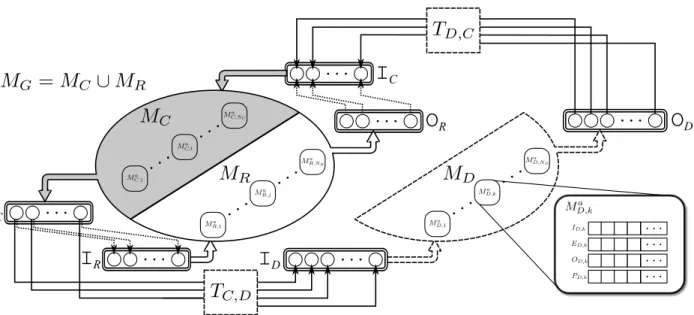
In order to formalize the sub-model interfacing method, we may define several model sets (see Figure
2). As proposed in the previous section, MG represents the set of N original atomic or coupled sub-models
constituting the ‘core-model’ (MG72 or MG92 in our case). This set, represented in Figure 2 as an ellipse, can
be partitioned into two subsets:
{
M
R, j}
⊆ M
{
G,i}
, j=1,…,NR including the sub-models that we wish toreplace (white part of the ellipse in Figure 2), and
{
M
C,l}
= M
{
G,i}
− M
{
R, j}
, l=1,…,Nc; Nc =N-NRcontaining the sub-models that will be conserved from the original model (gray part of the ellipse).
Furthermore, let
{
MD,k}
(truncated ellipse with segmented lines in Figure 2) be the set of k=1,…,ND new, more detailed models that we wish to integrate instead of MR. We may also define the following vectors:model v in MU, where U ∈ G, R, D,C
{
}
for the original (Guyton), replaced, detailed and conserved modelsets, respectively. These vectors will be useful for the definition of the interface between models in different sets. The proposed approach for replacing MR by MD and for interfacing MD with MC is the following:
1. Identification of the variables involved in the interaction of models in MC, MR and MD. Six sets can be
defined in this step, from the analysis of vectors
I
U ,vandO
U ,v. These sets contain the inputs and outputs of a given model set, which depend on outputs and inputs of models pertaining to a different set(rounded boxes with double lines in Figure 2).
I
R= I
{
R, j( )
n
: I
R, j( )
n
depends on O
C,l( )
m
}
,O
R= O
{
R, j( )
m
: I
C,l( )
n
depends on O
R, j( )
m
}
,I
D= I
{
D,k( )
n
: I
D,k( )
n
depends on O
C,l( )
m
}
,O
D= O
{
D,k( )
m
: I
C,l( )
n
depends on O
D,k( )
m
}
,I
C = I{
C ,l( )
n : IC ,l( )
n depends on an element inO
R}
, andO
C = O{
C ,l( )
m : an element inI
R depends on OC ,l( )
m}
(3)
where n and m are the indexes of each input or output vector, respectively. During the model replacement procedure, the links between
O
R andI
Cand betweenO
C andI
R (dotted arrows inFigure 2), will be removed. M2SL provides tools to automate this first step.
2. Perform a whole-model sensitivity analysis (on models MG72 or MG92) to study the response of their main
variables with respect to all the model parameters and perform module-based sensitivity analyses on each model in MR to analyze OR,j with respect to variations in IR,j. This step is crucial i) to better
understand the physiological properties and limitations of the global model and of each original sub-model, ii) to identify parameters and variables presenting the strongest and weakest interactions, since this information is useful to determine the elements in MR and MD for a particular problem, and iii) to
evaluate the impact of the integration of MD into the whole model, by comparing results of this step with
a sensitivity analysis performed after integration of MD. Section 2.2.1 will describe the methods applied
in this paper for these whole-model and module-based sensitivity analyses.
3. Design, implementation, and evaluation of the interface between models in MDand models in MC. This
step is particularly difficult, since it may require the definition of appropriate input-output
transformations (TC,D or TD,C) allowing to interface elements in
O
D with elements inI
C and betweenO
C andI
D. These transformations are illustrated as segmented boxes in Figure 2. Furthermore,specific simulation methods and parameters for models inMD should also be defined, since they may be
developed under different formalisms or present significantly different dynamics. Section 2.2.2 presents the proposed model interaction approach.
It should be noted that the method presented above may be applied to any coupled model, even if it is a sub-module of a higher-level coupled model or if models in MD and MR contain coupled models.
Insert Figure 2 here
2.2.1. Whole-‐model and module-‐based sensitivity analyses
As stated above, we carried out two kinds of sensitivity analyses: i) a whole-model analysis of the response of the main variables to changes in the model parameter values, and ii) a module-based sensitivity analysis of all the OR,j to changes in IR,j for each sub-model in MR. For both cases, a complete sensitivity
analysis would involve testing the effects of successive changes in several model parameters or input
variables, since physiological adjustments are of this sort, but this would be a daunting undertaking given the number of possible combinations. In the present study, the sensitivity analysis is focused on the effects of perturbations of one parameter or input variable at a time, based on the screening method of Morris (Morris, 1991). This method was chosen because it provides not only a measure of the effect of each parameter on each variable, but also gives information on nonlinearities and interactions among variables and parameters, by means of the analysis of the mean (µ) and standard deviation (σ) of a set of normalized measures of parameter (or input) sensitivity, defined as "elementary effects". In this analysis, µ indicates the relative sensitivity of a given output to a specific parameter (in the global model) or input variable (for isolated modules), and σ gives a measure of the dependence of the sensitivity on the values of the other inputs. Module-based sensitivity analysis was performed by directly applying the Morris method, as described in his paper. More details on the Morris screening method are presented in Appendix A.
Briefly, concerning the whole-model sensitivity analysis, a Monte Carlo approach was applied by repeating the Morris method a large number of times (i.e., 1000 here) for a number of selected parameters; since many of the more than 200 model parameters have no physiological significance (i.e., many are for internal looping control or represent technical implementation details), we selected 96 parameters for their putative physiological relevance in the model. Thus, this process produced 192,000 'virtual individuals' with randomized parameter values. For each instance, the values of all selected parameters were chosen at random within a viable range, and the simulation was run to steady state (4 weeks of simulated time) before effecting a parameter perturbation (10% of the valid range for each given parameter, see below). This provides i) a large, steady state virtual population that can be explored statistically for relationships among the model parameters and variables, and ii) a one-at-a-time parameter sensitivity analysis giving the mean (µ) and standard deviation (σ) for the normalized effect of each of the selected model parameters on each of the model output variables. Given the nonlinearity and the strong interdependence of the system, we tracked the sensitivity effects over time, focusing both on mid-term changes (5 minutes, 1 hour) and longer-term effects (1 day and 1 week). This raises the question of following up with optimization studies in search of, for example, unsuspected scenarios leading to hypertension, but these lie outside the present work. We also carried out a covariance analysis (results not given here) that gives valuable information about the
interdependencies of parameter effects on any given variable, thus providing pointers for a more physiologically applicable study of the effects of concomitant changes of several parameters.
2.2.2. Model interaction approach
As stated above, the first step to couple models in MD and MC is to define specific input-output linear or
non-linear transformations: IC,l
( )
n = T l,n D,C(O
D, P l,n TDC), IC,l( )
n ∈I
C and ID,k( )
n = Tk,nC,D(O
C, P k,n TCD), ID,k( )
n ∈I
Dwhere PT• are the parameters characterizing each transformation. For example, let
O
C ,lD ⊆O
D be the elements inO
D connected to IC,l( )
n . In the simplest case, whenO
DC ,l = 1, when the corresponding models are defined under the same formalism, and when these variables share the same physical units and temporal resolutions, the application of TD,Cl,n is trivial and the corresponding elements l are defined as the identity
function. When this is not the case (heterogeneous models), problem-specific transformations have to be designed, although some general cases can be identified. For example, if
O
DC ,l > 1, such as in the case of different spatial resolutions of the same physical variable, an up-scaling method (such as homogenization or variable aggregation) will be applied, through Tl,n
D,C, to the elements on
O
DC ,l. A simple example of such a transformation is the application of an instantaneous weighted sum of the elements on
O
DC ,l, as in (Auger and De La Parra, 2000), with the coefficients of this transformation represented in Pl,n
TCD. A similar approach can be applied when
O
DC ,l = 1, and when both variables share the same physical units, but the temporal resolution of variables in
O
DC ,lis much higher. In this case, the scaling transformation can be applied in the time domain by means of filtering and subsampling (Hernández et al., 2009). Down-scaling methods can be applied when defining Tk,n
C,D, in particular when one output in
O
C should be connected to many inputs inI
D. A variety of up-scaling or down-scaling methods have been proposed in the literature (Auger and Lett,2003; Lischke et al., 2007). The complex nature of the physiological systems, however, makes the application of analytic methods difficult, especially when coupling models defined under different mathematical formalisms.
Yet another case is when the physical units of variables in IC,l
( )
n andO
D C ,lare different. In this case, Tl,nD,C
will additionally include the unit conversion process. However, in some cases, these variables may be represented in relative or arbitrary units, requiring the estimation of specific parameters Pl,n
TCDin order to define an appropriate model interaction. Section 3 presents several examples of the definition of such transformations, when integrating heterogeneous models within the Guyton models. These transformations are implemented in M2SL through specific input-output "coupling objects".
The second step of the coupling method includes the definition of appropriate simulators and simulation parameters for each model in MD and MC. This step is particularly important when the dynamics of these
models are significantly different or when the models have been developed under different mathematical formalisms. In order to address this problem, M2SL is based on the co-simulation principle, in which each model is associated with a specific simulator, adapted to the mathematical formalism of the corresponding model. These simulators can be represented as:
O
U ,v= S
U ,v hM
U ,vh, P
U ,vS, F
U ,v(
)
, (4)where
S
U ,vh is the simulator for modelM
U ,vh , h ∈ a,Coup{
}
for atomic or coupled models, respectively, andP
U ,vS is a vector defining the simulation parameters (including specific model parameter values, initialconditions, integration step-size for continuous models, etc.). Each
S
U ,va may thus use a different simulation method, with different simulation time-steps. The coupling of all atomic models is performed within theMCoup model that contains them, through an
S
U ,vCoup. Three different strategies for coupling and synchronizing all atomic models are implemented in
S
U ,vCoup objects: i) simulation and synchronization with a unique, fixedtime-step; ii) adaptive simulation of atomic models and synchronization at the smallest time-step required by any of the atomic models; and iii) synchronization at a fixed time-step and atomic simulation with
independent, adaptive time-steps. More details on these different simulation strategies, with examples on the Guyton model, are presented in (Hernández et al., 2009).
3. Results
3.1.
Whole-‐model sensitivity analysis
Using the Morris method described above, we carried out an extensive sensitivity analysis using the 1992 version of Guyton's model, implemented by us to allow looping over the various model parameters. Here, p = 50, and the size of the perturbations, ∆, was taken to be 5/(p-1); that is, for each parameter, the range of values between its minimum and its maximum values was split into 50 slices, and the size of the perturbation ∆ corresponded to one-tenth of this range. In our MG92, we have 296 model variables of interest
and 96 input parameters of physiological interest (for which we defined workable minima and maxima based, as far as possible, on physiological criteria from the experimental and clinical literature), and r =
1000.
For a given xj, we start with a randomized input vector
ˆx
and evaluate the output variablesˆy
beforeand after increasing xj by ∆. These results give a value of eeij for each of the yi output variables at each
is repeated r times to produce a random sample of r elementary effects of xj. Then, this process is repeated
for each of the Nx input parameters. The total computational cost is 2r times Nx = 192,000 simulations; each of these represents a virtual patient. The frequency distribution of the blood pressure variable (PA) was approximately normal, and simulated PA values ranged from 80 to 189 mmHg, of which 109,266 were "hypertensive" (steady state PA > 106.6 mmHg) and 82,734 were normotensive (steady state PA ≤ 106.6 mmHg).
We also carried out a covariance analysis (results not given here) that gives valuable information about the interdependencies of parameter effects on any given variable, thus providing pointers for a more
physiologically applicable study of the effects of concomitant changes of several parameters. These results also provide a good starting point for the use of such a core-model for systematic in silico exploration of possible new drug effects, hypotheses about successive perturbations leading to disease states, or alternative treatment strategies. As stated above, an additional outcome is the production of a virtual population, where each virtual individual is characterized by a set of parameter values and the associated outputs (analagous to
phenotypes). Specific real-world patients could be associated with one or more of these virtual individuals by
doing a sort to match available clinical indicators against the values of identifiable model parameters and variables (e.g., arterial pressure, cardiac output, rate of glomerular filtration, hematocrit, blood viscosity,…)..
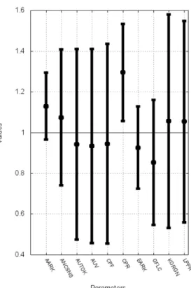
Since the results of this global analysis are voluminous and lie outside the main focus of the present paper, we give here, in Figure 3, just a sample of the results using the virtual populations, namely, an indication of the 10 parameters whose values were at least 5% different in the normotensive and hypertensive subpopulations.
Insert Figure 3 here.
Certain of these parameters come as no surprise; e.g., one expects to see that the afferent and efferent glomerular arteriolar resistances (AARK and EARK, resp.), the glomerular filtration coefficient (GFLC), and the level of salt intake in the diet (NID; see also section 3.3). The others, however, invite deeper reflection and will be analyzed in more depth in subsequent focused studies. Such studies are beyond the scope here; indeed, the results shown in Figure 3 should not be interpreted too hastily. The reader will realize that although the means of these 10 parameters were significantly increased or decreased in the virtual patients with hypertension, one cannot conclude that any particular combination of them was systematically altered in particular virtual individuals. The sorting out of interesting relationships on this score is the object of ongoing work to be published separately.
3.2.
Integration of an elastance-‐based pulsatile heart model
Heart failure (HF) is a multifactorial syndrome that may be caused by a number of genetic and environmental factors. This syndrome is mainly characterized by a reduced cardiac output, due to analteration of the cardiac mechanical properties during systole and/or diastole and, in some cases, its electrical properties (intra or inter-ventricular desynchronization of the cardiac electrical activation). Regulatory mechanisms are established in the early stages of HF to compensate for the reduced cardiac output. These mechanisms include an elevated sympathetic tone (which increases heart rate, blood flow and blood pressure) and a remodeling of the ventricular tissue. Even if these regulatory mechanisms can compensate for short-term lack of contractility, they become deleterious in the mid- to long-term and may increase the mechanical ventricular dysfunction, causing a permanent increase in pre-load and afterload, pulmonary or peripheral edema, decreased renal output and dyspnea on exertion (McMurray, 2010).
The Guyton models include simplified representations of a number of regulatory mechanisms that are central to the analysis of HF (Figure 1). However, the cardiac module in MG72 and MG92 is a non-pulsatile model
providing only mean values of the main hemodynamic variables via a static cardiac function curve. This is an important limitation when studying HF for several reasons: i) the significant modifications of this syndrome on ventricular contractility during systole, diastole, or in the presence of a biventricular
desynchronization cannot be represented, ii) some useful clinical variables, such as the maximum value of the arterial pressure derivative (dP/dtmax) or the evolution of the systolic and diastolic pressures, cannot be simulated, and iii) a more realistic representation of short-term regulatory loops (such as the baroreflex) requires these pulsatile variables.
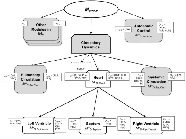
In this sense, the general method proposed in section 2.2 will be applied here to replace the original, non-pulsatile cardiac sub-model of MG72 with an elastance-based pulsatile model of the heart, including interventricular interaction through the septum (MG72-P). In this case, the set MR is the Heart sub-module, located within the Circulatory Dynamics coupled module.
O
C= {PLA (left atrial pressure), PA (arterialpressure), PRA (right atrial pressure), PPA (pulmonary arterial pressure), AUR (autonomic effect on heart rate) and AUH (autonomic effect on heart strength)} and
I
C= {QMI (mitral flow), QLO (left ventricular outflow), QTR (triscupid flow), QRO (right ventricular outflow)}. Figure 4 depicts the integration of the new models within the Circulatory Dynamics coupled module and within MG72.Insert Figure 4 here
3.2.1.
Sensitivity analysis of the Circulatory dynamics module
An input-output sensitivity analysis has been applied to the Circulatory Dynamics sub-models of the MG72
and MG92 models in order to optimize the design of the new pulsatile model and define the model integration
the Circulatory Dynamics module has 15 outputs, it has Nx = 16 inputs in MG72 and Nx = 23 in MG92. The
Morris screening method, as described in (Morris, 1991), has been applied with p = 20 and Δ = p/(2(p-1))=0.526. The total number of simulations performed for this analysis was n = 5‧Nx‧(k+1), where Nx is the total number of inputs, as defined earlier. The simulations were run 1 min to obtain a steady state before effecting an input perturbation. Results are represented by means of µ-σ planes, where µ and σ are, respectively, the absolute mean value and the standard deviation of the set of elementary effects (eeij)
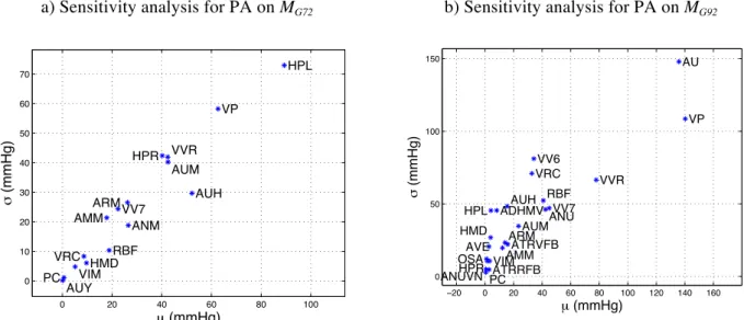
computed for each input j of each Circulatory Dynamics module. Insert Figure 5 here
Figure 5 (a) and (b) depict the sensitivity analysis results on the mean arterial pressure obtained respectively
from the MG72 and MG92 models. In both cases, the simulated arterial pressure is particularly sensitive to
modifications of: i) total blood volume, ii) the autonomic modulation of the cardiac activity and iii) vessels contractile state. The Circulatory Dynamics output plasma volume (VP, both in MG72 and MG92) is one of the
most significant factors, since the liquid component of blood directly affects the total blood volume. Furthermore, the vascular volume caused by relaxation (VVR), also has an important influence on the arterial pressure, since it directly reflects constriction of venous vessels, driven by autonomic activity. Variables representing the autonomic nervous system (ANS) modulation (AU for MG92 and AUH and AUM
on both MG72 and MG92) have a significant influence on the simulated arterial pressure, since it regulates
cardiac contractility, heart rate and peripheral vasoconstriction. Particular attention will be paid to the integration of these variables into the new pulsatile model. The main differences between the two versions of the model concern the influence of hypertrophy effects on the ventricle (HPL and HPR), which is more important in the MG72 model. These variables will not be coupled to the pulsatile cardiac model, since new
state variables will allow for the modification of different aspects of cardiac contractility in a more detailed fashion.
3.2.2.
Integration of the new cardiac sub-‐module
In this section, we first describe the proposed cardiac pulsatile model (MD) and then the coupling approach
between this model and those in MC. The set MD is constituted here of one coupled model, including atomic
models which represent the four cardiac valves, two pulsatile ventricles, and the interventricular septum (see
Figure 4). Cardiac valves are represented by modulated resistances. Atomic models representing both
ventricles are described by elastic chambers (Smith et al., 2004). One cycle of ventricular elastance is given by:
e(t) = AeB(te⋅HR 60−C )
(5) where A = 1, B = 250s-2 and C = 0.27s are parameters that define the function’s profile, and variable t
e
corresponds to the time elapsed since the last ventricular electrical activation. Ventricular pressure-volume loops are characterized by the End Systolic Pressure-Volume Relationship (ESPVR) and the End Diastolic
Pressure-Volume Relationship (EDPVR), which can be defined as Pes(V ) = Ees(V − V0) and
Ped(V ) = P0(e
λ (V −V0)− 1). The end systolic pressure (P
es) is described as a linear relationship between the
volume (V), the volume at zero pressure (V0) and the end systolic elastance (Ees), while end diastolic pressure
(Ped) is defined by a non-linear relationship defined by the elastance of ventricular walls during diastole (P0)
and the curvature of the EDPVR (λ). The ventricular pressure-volume relationship can be defined as:
P(V ) = e(t)Pes(V ) + (1 − e(t))Ped(V ).
(6) The Smith model describes the interaction between the two ventricles through the interventricular septum by defining the left and right ventricular free wall volumes, as follows (Smith et al., 2004):
Vlvf = Vlv - Vspt (7)
Vrvf = Vrv + Vspt, (8)
where Vspt represents the volume modification due to septal dynamics. Pressures for the ventricles and the septum are described by applying equation (6) with specific elastance functions (5) for each case:
Plvf = elvf(t) Pes,lvf + (1 - elvf(t)) Ped,lvf
Prvf = ervf(t) Pes,rvf + (1 - ervf(t)) Ped,rvf
Pspt = espt(t) Pes,spt + (1 - espt(t)) Ped,spt
(9) The relation between the septum, the left, and the right ventricles is defined by Pspt = Plvf – Prvf.
To summarize, the inputs of the pulsatile model are
I
D= {te, PA (arterial pressure), PLA (left atrialpressure), PRA (right atrial pressure) and PPA (pulmonary arterial pressure)} and its outputs
O
D = {QMI(flow through the mitral valve), QLO (flow through the aortic valve), QTR (flow through the tricuspid valve), QRO (flow through the pulmonary valve)}. In order to couple this model with elements in MC, these
I
D andO
D should be connected to the corresponding elements inO
C andI
C, defined previously, throughcoupling objects integrating appropriate transformations TD,C and TC,D.
The coupling of hemodynamic variables (pressures and flows) is relatively simple in this case, since they are represented with the same physical units in
I
D,O
D,O
C andI
C. However, the temporal resolution of thesevariables in
I
D andO
D is significantly different. A first approach, based on the application of a filter for thetransformation of these variables has been presented in a previous work (Hernández et al., 2009). The objective here is to preserve this higher temporal resolution within models in MC, while assuring the stability
of the whole coupled model. This point requires the appropriate transformation and coupling of the autonomic regulation variables within the cardiac model and the Systemic Circulation module. Three coupling variables are defined in MG72 for autonomic regulation of the cardiac activity: AUR, AUH and AUM, concerning respectively the regulation of: i) heart rate (chronotropic effect), ii) cardiac contractility (inotropic effect) and iii) systemic resistance. These variables are defined in arbitrary units. Transformations
TC,D were thus defined for these variables with the following general equation:
XT = SX⋅ X − 1
(
)
+ BX (10)where X stands for AUR, AUH and AUM and SX and BX are, respectively, sensitivity and baseline
AURT, AUHT and AUMT should be further processed and coupled to the pulsatile model before performing
the estimation of appropriate parameter values for SX and BX.
In order to integrate the chronotropic effect, an Integral Pulse Frequency Modulation (IPFM) model (Rompelman et al., 1977) was included within a transformation linking variable AURT (used as input to the
IPFM model) and variable te of equation (5). The IPFM model generates a pulse corresponding to the
electrical activation instant used for all elastances (elvf, ervf and esept). Concerning the integration of the
inotropic effect, variable AUHT was used to modulate the ventricular elastance as follows:
Ees = AUHT ⋅ Ees 0 (11)
where Ees0 is the basal value for the end-systolic elastance, which is an internal parameter of MD.
Furthermore, in order to assure the stability of the new global, coupled model, the original AUM variable, controlling the systemic resistance in the Systemic Circulation sub-model, was replaced by the transformed AUMT variable.
Finally, appropriate values for parameters PTCD = [SAUR, SAUH, SAUM, BAUR, BAUH, SAUM] were estimated by applying an optimization algorithm configured to minimize an error function defined between the
simulations obtained from MG72 and those obtained from MG72-P. A known benchmark simulation of the Guyton models was used during the parameter optimization process, which consists of doubling the resistance of non-renal circulation, such as the one that can be caused by the injection of vasoconstrictor drugs, at t=1min (Van Vliet and Montani, 2005). An evolutionary algorithm was used to minimize an error function ε, defined as:
ε = 1
N t=0
(
PAG 72−P(t) − PAG 72(t) + AUG 72−P(t) − AUG 72(t) + QLOG 72−P(t) − QLOG 72(t) + RsG 72−P(t) − RsG 72(t))
7 min∑
(12)where variables PAG72, AUG72, RsG72 and QLOG72 correspond to the original Guyton output variables and
PAG72-P, AUG72-P, RsG72-P and QLOG72-P stand for the output of the Guyton model including pulsatile
ventricles. PA, AU, Rs and QLO are respectively the mean arterial pressure, the autonomic activity (which is not an input of the Circulatory Dynamics module on MG72), the resistance in non-renal circulation and the cardiac output.
3.2.3.
Simulation results and discussion
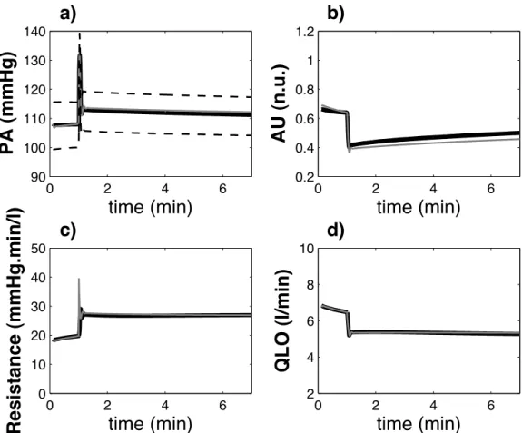
Figure 6 shows the comparison between the simulations obtained with MG72 and MG72-P for a sudden increase
of global peripheral resistance (simulation experience used during the parameter identification stage). In order to compare simulation results from both models, each pulsatile variable obtained from MG72-P was
post-processed to obtain beat-to-beat mean, systolic and diastolic values, with the following procedure: i) detection of each beat, ii) estimation of the minimum and maximum (diastolic and systolic) values for each beat and iii) estimation of the mean value by integrating each variable on the time support associated with each beat and dividing by the cardiac period. These beat-to-beat variables are superposed to the original MG72
variables in Figure 6. A close match between the results obtained from MG72 and the post-processed MG72-P
variables can be observed. In both cases, the rise of the systemic resistance provokes a transient increase of arterial pressure level that rapidly leads to a decreased activity of the renin-angiotensin and the sympathetic systems. As a consequence, arterial pressure level is stabilized at a slightly higher value, and cardiac output falls to a lower level. In addition, the evolution of the systolic and diastolic values of the arterial pressure (segmented lines on Figure 6 a) can be analyzed from MG72-P. An example of the pulsatile hemodynamic
variables generated by MG72-P is shown in Figure 7. These variables present values that are consistent with
known physiological data.
Insert Figure 6 here Insert Figure 7 here
The reproduction of the in silico experiments described in (Guyton et al., 1972), which has already been studied for our implementation of MG72 in (Thomas et al., 2008), has also been performed with MG72-P. As an example, results obtained from benchmark experiment 1 in (Thomas et al., 2008) provided a mean relative root mean squared error (rRMSE) equal to 0.0203 when comparing the set of output variables of MG72 with
MG72-P, which is an acceptable result. rRMSE for the most sensitive variables are the following: extracellular fluid volume (VEC), rRMSE = 0.011; blood volume (VB), rRMSE = 0.012; sympathetic stimulation (AU), rRMSE = 0.01; heart rate (HR), rRMSE = 0.012 and arterial pressure (PA), rRMSE = 0.01.
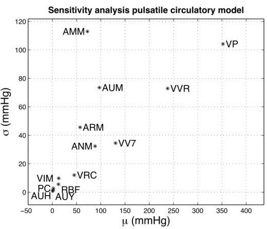
Finally, the impact of the integration of the pulsatile model within the original Circulatory Dynamics sub-model was analyzed through a new sensitivity analysis. Figure 8 shows the Morris input-output sensitivity results on arterial pressure. Compared to the sensitivity analysis performed on the Circulatory Dynamics sub-model of the original MG72 model (Figure 5a), the most sensitive variables are still the plasma volume
(VP), the autonomic regulation of vasoconstriction on arteries (AUM), and the vascular volume caused by relaxation (VVR). It is possible to observe an increased sensitivity to inputs that modulate the systemic resistance: ANM (general angiotensin multiplier effect, ratio to normal), ARM (non-muscle global
autoregulation multiplier), and AMM (overall multiplier factor for muscle autoregulation). This difference can be explained by the fact that the new cardiac model integrates a more realistic response to variations in preload and afterload.
The modifications performed in this section are an important initial step towards the adaptation of the Guyton models for a systemic analysis of heart failure. In previous work, we have proposed hybrid, tissue-level electromechanical models of cardiac function and parameter identification methods that are able to reproduce regional echocardiographic strain data from patients suffering from HF (Fleureau et al., 2009; Le Rolle et al., 2008). However, the hemodynamic boundary conditions of these models were not realistic and
none of the short or long-term regulatory mechanisms of the cardiovascular system were integrated. Current work is thus directed to couple these models with the Guyton models, by applying the method proposed in this paper in order to study new diagnostic and therapeutic approaches to heart failure. Indeed, preliminary results integrating a model of a cardiac resynchronization pacemaker with a hybrid elastance-based cardiac model, coupled with systemic and pulmonary circulations, have shown the importance of the joint analysis of these systems for the correct definition of patient-specific stimulation parameters (Tse Ve Koon et al., 2010). Section 3.3 below is devoted to the improvement of another important subsystem of the Guyton models for the analysis of this pathology (as well as hypertension), namely the renin-angiotensin system.
3.3.
Integration of a model of the endocrine renin-‐angiotensin system
In normal CVR physiology, homeostasis of body sodium and arterial pressure (PA) strongly relies on the renin-angiotensin system (RAS). In CVR disease, the paramount role of RAS is substantiated by a systematic involvement in hypertension, heart and kidney failure, atherosclerosis, diabetes and metabolic syndrome (Hsueh and Wyne, 2011). As a consequence, RAS is a primary target for pharmacological agents (ACE, angiotensin-converting enzyme, inhibitors, angiotensin receptor blockers, direct renin inhibitors)— and dietary maneuvers such as sodium restriction—directed against such pathologies (Atlas, 2007). For instance, RAS activation associates with higher risk of cardiovascular events, whereas drug action (e.g. ACE inhibition), as well as sodium restriction, reduces cardiovascular mortality and slows kidney disease progression (Brown, 2007).RAS is an endocrine cascade that starts with renin (REN) production by the renal juxtaglomerular
apparatus (JGA), in response to a decrease in PA, natremia and/or volemia. REN is an enzyme which
converts circulating angiotensinogen (AGT, a liver-derived glycoprotein) into angiotensin I (Ang I). This inactive peptide is then converted by ACE to angiotensin II (Ang II). Ang II is the major RAS effector, adjusting PA, salt (and water) via i) arterial and venous vasoconstriction, ii) renal sodium reabsorption, iii) thirst and salt appetite, and iv) secretion of aldosterone (for a review, see (Atlas, 2007); for tissue-specific aspects, see (Paul et al., 2006)).
In the original MG72 model (and MG92), the treatment of RAS is restricted to the ANM signal
(angiotensin multiplier effect on vascular resistance, ratio to normal), modulating peripheral resistance and aldosterone production (Guyton et al., 1972). Encompassing both REN and Ang II, ANM is an ‘average’ measure of RAS activation, produced by a dedicated module (Angiotensin control) under the inhibitory influence of the ‘macula densa’, MD (via GF3 signal in MG72), a key element in the feedback control of
glomerular filtration rate. As a consequence, the original Guyton models contain no specific inclusion of those RAS regulators and elements that are widely targeted by pharmacology and clinics (Atlas, 2007; Brown, 2007), i.e.: i) RAS biochemical actors (AGT, REN, Ang I, ACE, Ang II), and ii) established
physiological regulators of renin production (other than MD), namely PA, Ang II, and renal sympathetic nerve activity (RSNA). Thus, the improvement of RAS description constitutes a sine qua non step toward the rational exploitation of such models in human pathology, pharmacology or clinics.
Contrary to cardiac or autonomic CVR regulation, there are few dedicated models of endocrine systems, especially for the RAS. To our knowledge, two ‘stand-alone’ RAS models have been proposed. Focusing upon primary aldosterone-induced hypertension, Hsieh and coll. developed a RAS model to predict renin and aldosterone changes under short-term diuretic treatment (Hsieh et al., 1990). Takahashi and coll. developed a steady-state RAS model of reactions leading to Ang II formation, combined with gene expression of RAS-elements (AGT, REN, ACE) (Takahashi et al., 2003). In addition, as in the Guyton models (Guyton et al., 1972; Montani and Van Vliet, 2009), RAS descriptions have been proposed as modules integrated within CVR circulatory models (Ikeda et al., 1979; Karaaslan et al., 2005; Uttamsingh et al., 1985). However, all these models lack several of the following features of RAS: realistic system dynamics, explicit enzymes and kinetics, representation of the main renin regulators (PA, Ang II, MD, and RSNA), validation against human clinical data.
In order to fill these gaps, we recently developed a realistic model of RAS for integration into MG72
(Guillaud and Hannaert, 2010). In brief, our model integrates the following missing elements, i.e., i) biochemical elements (from AGT to Ang II) in a Plasma model, ii) physiological renin regulators, in a JGA model. After parameter optimization, the whole construct was validated against human data (Guillaud and Hannaert, 2010).
Here, we present the modular organization of the new MG72-RAS module, the sensitivity analysis of the
original and new models (in terms of RAS and kidney function), and simulation experiments demonstrating the benefits of the new RAS in terms of physiological behavior of the integrated CVR model.
3.3.1. Sensitivity analysis of kidney and RAS-‐related modules
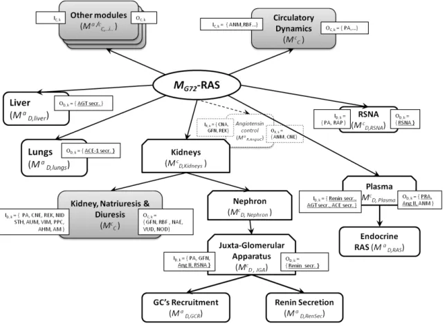
Figure 9 shows, in comparison with MG72, how the additional models were organized and integrated
into the new MG72-RAS. Referring here to results obtained at one simulated week (steady-state, NID ≈ NOD),
the Morris screening method (‘µ-σ plane’ of elementary effects) was used to explore the I/O sensitivity of the kidney model (Kidney, Natriuresis & Diuresis module, Mc
C,KDN ; Δ = 0.526 , p = 20, k = 10 (10 inputs), r =
550 simulations) and the RAS model (Angiotensin control; Δ = 0.526 , p = 20, k = 3 (3 inputs), r = 60 simulations). In MG72, for the kidney model we observed that:
• glomerular filtration (GFN) was primarily modulated by SNA-dependent arteriolar tone (AUM), PPC (plasma colloids), and PA; these 3 variables exhibited interdependent influences upon GFN (σ > 0); other inputs had negligible effects on GFN (i.e. close to [0,0] in the µ-σ plane);
• NAE and NOD were equally and interactively influenced by AM, AUM, PA, PPC, NID, and STH, while VUD depended on PA, PPC, and REK;
• much like GFN, RBF was essentially modulated by AUM and PPC, interactively. For theRAS model (Mc
R,AngioC), we observed that ANM was strongly and interactively modulated by
GFN and REK, and to a lesser extent by CNA.
Sensitivity analysis of MG72-RAS: Focusing on the ‘activation state’ of the new RAS, I/O sensitivity analysis
showed that the introduction of PA as a regulator led to its quantitative preponderance upon ANM output (the other inputs collapsed around 0,0 in the µ,σ plane). On the other hand, CNA (while conserving its expected sole influence, see above) lost some ‘quantitative’ influence upon CNE, possibly due to a ‘dilution effect’.
3.3.1.
Simulation results and discussion
As mentioned, one essential function of RAS is to contribute to PA, natremia, and body fluids homeostasis. In this process, renin catalyzes the first step in the RAS cascade, in fine leading to sodium retention and adjustment of PA and volemia. In this physiological context relating RAS to sodium intake and PA regulation, we performed simple in silico experiments in order to evaluate the putative gains brought about by the presence of new RAS in Guyton’s circulatory model.
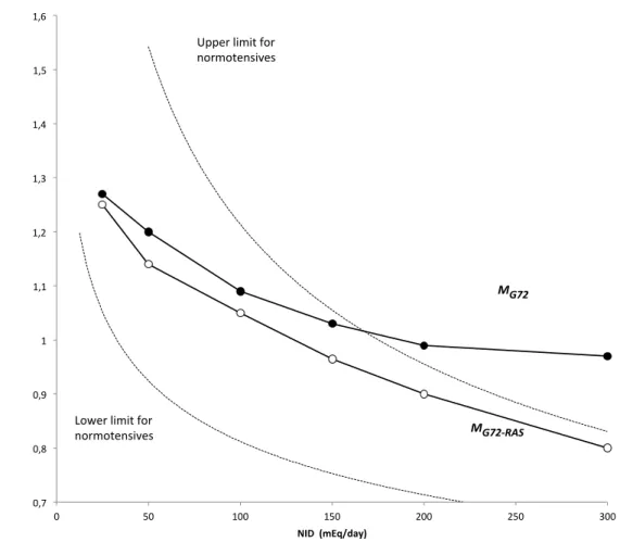
The steady-state dependence of plasma renin activity (RA), a measure of the RAS activation, on natriuresis (RA=f(NOD), i.e. the so-called ‘Laragh’s nomogram’), is a well-established observation (Laragh, 2001). Thus, we compared RAS activity of MG72 and MG72-RAS models as a function of NID (or NOD, at
steady-state): the ANM factor was used for comparison because it is the sole RAS variable common to both models. Figure 10 plots ANM factor versus NID. In the clinical setting, the referred biological variable is plasma RA: in order to position model outputs vs. ‘real’ plasma RA values, we also plotted lower and upper limits for normotensive patients, as ANM-equivalents, recalculated from (Laragh, 2001)(see legend of
Figure 10). Globally, it can be seen that both models produce the known and expected inverse, curvilinear
relationship between sodium input and RAS activation (Laragh, 2001; Laragh, 1995). However, the new model performs better than the native one, for two interdependent reasons. First, MG72-RAS outputs are well
confined within the operational definition of normal values (dotted lines on Figure 10), whereas MG72 ANM
outputs fall outside the physiological range, beyond 150 mEq/d. Second, the new construct appears about 50 % more ‘responsive’ to sodium input than the original, since ANM varies in a 0.45 range (0.80-1.25), instead of 0.30 (0.97-1.27) for MG72. In particular, whereas ANM/MG72 was practically unable to respond to
NID increases beyond 150-200 mEq/d, as opposed to observed clinical behavior (see Figure 10, upper and lower limits, as dotted lines), the new ANM signal proved able to do so: in the 150-300 mEq/d NID, the average ANM slope of the new model is 3-fold higher than the original one (0.11 vs 0.04 (100 mEq/d)-1). In
the present epidemiological context of excess sodium intake, this is of importance (Smith-Spangler et al., 2010).
The introduction of the new RAS module rendered the CVR circulatory-blood pressure homeostasis model more responsive, and over a wider range of sodium intake (10-300 mEq/d) known to be influential and patho-physiologically relevant (Laragh, 2001). In large part, this is due to the introduction (in addition to MD signal) of three key physiological REN controllers: the inhibitory PA and Ang II, on the one hand, and the stimulatory RSNA on the other hand. Indeed, an exploratory numerical analysis of the individual contributions of the four signals to NID-induced ‘renin modulation’ showed that Ang II (inhibitor) and RSNA (activator) dominate the response in the 30-300 mEq/d NID (data not shown). This further illustrates the gain brought about by the new RAS. One known system-level characteristic of the RAS is its baseline state of tonic inhibition, according to a dynamic balance between inhibitory (PA, MD, Ang II) and
stimulatory (RSNA) influences. Obviously, this could not be accomplished by MG72 since in that model only
MD (GF3 signal) controls RAS (ANM factor).
This observation points out the relevance and potential of the advocated ‘progressive systems physiology’ approach in the CVR context of and hypertensive patho-physiology since: (i) it is known that one major action of β-blockers to reduce blood pressure involves the inhibition of RSNA, thus reducing renin release (Brown, 2007), and (ii) more generally, the relative contributions of renin controllers (e.g., PA
vs MD signals, vs Ang II, etc) remain a subject of investigation, not only because these contributions are
intrinsically complex (e.g., the PA variable acts both via renal-arteriolar baroreceptor and via RSNA), but also because they depend on individuals and on their patho-physiological / clinical context.
In conclusion, the modular expansion of MG72 into MG72-RAS carried out brings in return a more
realistic model of the dynamic and coupled interactions that physiologically occur in the CVR system as it responds to sodium intake via the RAS. Because RAS and sodium are so tightly involved in hypertensive and CVR diseases, this opens the avenue toward pathophysiology, pharmacology and therapeutics, including variabilities and genetic polymorphisms (Jiang et al., 2009; Laragh, 2001; Laragh, 1995; Rudnicki and Mayer, 2009; Takahashi et al., 2003).
4. Conclusions and perspectives
With the emergence of integrative physiology and international projects such as the IUPS Physiome and the European Virtual Physiological Human (VPH), an increasing interest exists today towards the integration of different physiological models, which may cover different functions and be developed at various scales, under distinct mathematical formalisms. This paper presents a contribution to the formalization of the seldom-covered problem of the appropriate definition of the interfaces required to perform this model integration. It also proposes an approach to interface such heterogeneous models, by i) restructuring and modularizing the different models to be coupled, ii) analyzing their input-output sensitivity, and iii) defining appropriate input-output transformations and simulation methods.
The proposed approach has been applied to the extension and updating of the somewhat outdated but well-validated classic Guyton model in two ways: i) by replacement of one of its central modules with a
more detailed and up-to-date module, and ii) by insertion of a major new module whose details have been discovered over the decades since development of the classic model.
In the first instance, the original Circulatory dynamics module was replaced in order to transform the overall model so it could represent pulsatile blood pressure, whereas the original model represents only mean arterial pressure. This required installation of an adequate dynamic representation of the left ventricle, wholly missing from the original model. In the second instance, a recent and original detailed model of the RAS system was inserted into the global model. The effect of these modifications on local and overall model behavior is assessed using an extensive sensitivity analysis.
Both of these extensions bring significant new functionality to the model, enabling in silico exploration of physiological processes inaccessible to the original model. Both extensions also required a number of non-trivial adjustments to the other parts of the global model. The process of extension was made possible thanks to the powerful multi-resolution reformulation of the original Fortran model into C++ for solution using the M2SL package.
However, beyond the added functionality of the extended model, which still has to be validated, the central focus here is on the open, re-usability of the core-model approach, in the physiome spirit. Ours is not the first reformulation of the Guyton models—it has also been re-implemented in Matlab/Simulink
(Kofranek and Rusz, 2010; Kofranek et al., 2007) and more recently in Modelica (Kofranek, personal communication). It is also not the most advanced extension of the Guyton models—see for example the elaborate QCP/QHP/HumMod environment developed over the years by Guyton's collaborators (Hester et al., 2011). Nonetheless, given the unwieldy underlying description of the HumMod model (over 5000 variables, described in several thousand XML files) and the slow execution time and proprietary context of the Matlab/Simulink implementations, the project presented here is better geared to the goal of providing an open, collaborative context for continued extension and building up of integrated models of human
physiology. To this end, the computer code for the models described here will be made available through the Virtual Physiological Human Network of Excellence ToolKit. Moreover, the proposed multi-resolution approach differs from a purely Top-Down, Bottom-Up or Middle-out approach, as discussed in (Hester et al., 2011), since it allows to selectively up-scale or down-scale different components of the core-model as a function of the targeted application.
Some future extensions along the same lines have already been cited in the paper. Other possible extensions, which could be carried out by ourselves or others, could be: merger into the core-model of models to treat acid-base regulation in significantly more detail; replacement of the Kidney module to provide more explicit representation of known targets (i.e., ion channels, membrane transporters, hormone receptors, etc.) of drug therapy for hypertension and other kidney-related diseases; or better representation of the role of renal sympathetic nerve activity (Karaaslan et al., 2005), to name only three.
As the VPH/Physiome projects develop, an overarching goal is to work towards not only horizontal integration across organ systems, but also vertical integration across different levels of organization, from whole body down to cellular processes, metabolism, and relevant gene-regulatory processes to get at the
genotype-to-phenotype relationships (Houle et al., 2010; Hunter et al., 2010; Martens et al., 2009). The work described here is intended as a step in this direction.
Appendix A: The Morris sensitivity method
Given a deterministic system of variables y that depends on Nx inputs or parameters x1…xNx, i.e., ˆy = f ˆx
( )
; ˆy ≡ y(
1,..., yNy)
; ˆx ≡ x(
1,..., xNx)
; (13)we wish to estimate both the sensitivity of each yi to each xj,
∂ij
( )
ˆx =∂yi
∂xj (14)
and the degree to which the effect of xj depends on the values of xk, k ≠ j. To this end, we adopted the method
of Morris (Morris, 1991), which estimates not only the mean effect of each input or parameter on each model variable, but also the dependence of each parameter effect on variations of the other model parameters. A normalized measure of parameter sensitivity, the elementary effects, or eeij, is thus defined as the fractional
change of variable yi after a small perturbation of parameter xj, scaled by the corresponding parameter
changes. These elementary effects are thus defined as:
eeij=
yi( x1,...,xj+Δ,...,xNx)−yi( ˆx )
Δ (15)
where ∆ is the applied perturbation. Attention was restricted to a region of the parameter (or input variable) space ω, a regular Nx-dimensional p-level grid, where each xj takes values from {0, 1/(p-1), 2/(p-1), …,
(1-∆)}. Values for p and ∆, are defined for every analysis. We designate as Fij the distribution of eeij in a
number r of computational experiments, done with r randomized vectorsˆx(with each xj drawn at random
within the predefined grid). The resulting estimates of the absolute value of the mean µi,j and the standard
variation σi,j of the eeij, are indicators of which input parameters are important: a large value of µi,j indicates
that the parameter xj has a significant overall effect on the output, while a large value of σi,j is associated with
non-linear effects or with strong interactions with other parameters. Results from this sensitivity analysis can be represented graphically on the µ-σ plane.
Acknowledgments
We gratefully acknowledge the financial support of the French National Research Agency (ANR grants ANR-06-BYOS-0007-01 (SAPHIR), and ANR-08-SYSC-002 (BIMBO)), and the European Community’s Seventh Framework Program (FP7/2007-2013, grant agreement no. 223920, VPH-NoE). This work was also aided by discussions within the GdR STIC-Santé CNRS 2647 – INSERM.
Editor’s note
References:
Aslanidi, O.V., Colman, M. A., Stott, J., Dobrzynski, H., 2011. 3D virtual human atria: A computational platform for studying clinical atrial fibrillation. Prog. Biophys. Mol. Biol. pp-pp.
Atlas, S.A., 2007. The renin-angiotensin aldosterone system: pathophysiological role and pharmacologic inhibition, J Manag Care Pharm. 13, 9-20.
Auger, P. and De La Parra, B., 2000. Methods of aggregation of variables in population dynamics, Comptes rendus de l'Académie des sciences, Sciences de la vie. 323, 665-674.
Auger, P. and Lett, C., 2003. Integrative biology: linking levels of organization, Comptes Rendus Biologies. 326, 517-522.
Brown, M.J., 2007. Renin: friend or foe?, Heart. 93, 1026-33.
Clayton, R.H., Bernus, O., Cherry, E.M., Dierckx, H., Fenton, F.H., Mirabella, L., Panfilov, A.V., Sachse, F.B., Seemann, G. and Zhang, H., 2011. Models of cardiac tissue electrophysiology: Progress, challenges and open questions, Progress in Biophysics and Molecular Biology. 104, 22-48. Clayton, R.H. and Panfilov, A.V., 2008. A guide to modelling cardiac electrical activity in anatomically
detailed ventricles, Progress in Biophysics and Molecular Biology. 96, 19-43.
Fleureau, J., Garreau, M., Donal, E., Leclercq, C. and Hernández, A.I., 2009. A Hybrid Tissue-Level Model of the Left Ventricle: Application to the Analysis of the Regional Cardiac Function in Heart Failure, in: Berlin/Heidelberg, S. (Ed.), Functional Imaging and Modeling of the Heart. Springer-Verlag, pp. 258–267.
Guillaud, F. and Hannaert, P., 2010. A computational model of the circulating renin-angiotensin system and blood pressure regulation, Acta Biotheor. 58, 143-70.
Guyton, A.C., 1973. Circulatory Physiology I. Cardiac Output and Its Regulation, W.B. Saunders, Philadelphia.
Guyton, A.C., 1975. Circulatory Physiology II. Dynamics and Control of Body Fluid, W.B. Saunders, Philadelphia.
Guyton, A.C., 1980. Circulatory Physiology III. Arterial Pressure and Hypertension, W.B. Saunders, Philadelphia.
Guyton, A.C., Coleman, T.G. and Granger, H.J., 1972. Circulation: overall regulation, Annu Rev Physiol. 34, 13-46.
Hernández, A., Le Rolle, V., Defontaine, A. and Carrault, G., 2009. A multiformalism and multiresolution modelling environment: application to the cardiovascular system and its regulation, Philosophical Transactions Mathematical Physical & Engineering Sciences. 367, 4923-4940.
Hester, R.L., Iliescu, R., Summers, R. and Coleman, T.G., 2011. Systems biology and integrative physiological modelling, The Journal of Physiology. 589, 1053-1060.
Houle, D., Govindaraju, D.R. and Omholt, S., 2010. Phenomics: the next challenge, Nature Reviews Genetics. 11, 855-866.
Hsieh, B.S., Chen, Y.M., Wu, K.D., Kuo, Y.M., Hsieh, C.H. and Lee, P.W., 1990. A simulation study on renin and aldosterone secretions in primary aldosteronism, J Formos Med Assoc. 89, 346-9. Hsueh, W.A. and Wyne, K., 2011. Renin-Angiotensin-aldosterone system in diabetes and hypertension, J
Clin Hypertens (Greenwich). 13, 224-37.
Hunter, P., Coveney, P.V., de Bono, B., Diaz, V., Fenner, J., Frangi, A.F., Harris, P., Hose, R., Kohl, P. and Lawford, P., 2010. A vision and strategy for the virtual physiological human in 2010 and beyond, Philosophical Transactions of the Royal Society A: Mathematical, Physical and Engineering Sciences. 368, 2595.
Ikeda, N., Marumo, F., Shirataka, M. and Sato, T., 1979. A model of overall regulation of body fluids, Annals of Biomedical Engineering. 7, 135-166.
Jiang, X., Sheng, H., Li, J., Xun, P., Cheng, Y., Huang, J., Xiao, H. and Zhan, Y., 2009. Association between renin-angiotensin system gene polymorphism and essential hypertension: a community-based study, J Hum Hypertens. 23, 176-81.
Joshi, H., Singharoy, A. B., Sereda, Y. V., Cheluvaraja, S., Ortoleva, P. J., 2011. Multiscale Simulation of Microbe Structure and Dynamics. Prog. Biophys. Mol. Biol.pp-pp.
Karaaslan, F., Denizhan, Y., Kayserilioglu, A. and Gulcur, H.O., 2005. Long-term mathematical model involving renal sympathetic nerve activity, arterial pressure, and sodium excretion, Ann Biomed Eng. 33, 1607-30.