Characterization of the exhaust gas condensate pH values of gasoline engines

Characterization of the Exhaust Gas Condensate

pH Values of Gasoline Engines

by

Lakshya Jain

Bachelor of Technology in Mechanical Engineering

Indian Institute of Technology Kharagpur, 2014

Submitted to the Department of Mechanical Engineering

in partial fulfillment of the requirements for the degree of

MASTER OF SCIENCE IN MECHANICAL ENGINEERING

at the

MASSACHUSETTS INTITUTE OF TECHNOLOGY

MASSACHUSETTS INSTITUTE OF TECHNOLOGY

SEP 13 2016

LIBRARIES

ARCHIVES

September 2016

C 2016 Massachusetts Institute of Technology. All rights reserved.

Signature redacted

Department of Mechanical Engineering

August 8, 2016

Certified by_

Signature redacted

Wai K. Cheng Professor of Mechanical Engineering; Director, Sloan Automotive Laboratory Thesis Supervisor

Accepted

Signature redacted

Rohan Abeyaratne

Quentin Berg Professor of Mechanics

Chairman, Committee on Graduate Students

Author

Characterization of the Exhaust Gas Condensate

pH Values of Gasoline Engines

by

Lakshya Jain

Submitted to the Department of Mechanical Engineering

on August 8, 2016, in partial fulfillment of the requirements for the degree of

Master of Science in Mechanical Engineering

Abstract

Exhaust Gas Recirculation has been used in gasoline engines to reduce NOx formation and

part-load throttle loss for many years. More recently, there is a trend towards down-sizing

and turbocharging engines as the strategy helps to improve fuel economy. Cooled low

pressure EGR complements down-sizing-turbocharging in direct injection gasoline engines

and has the potential to further improve efficiency. When exhaust gas gets cooled down

below its dew point in an EGR cooler, the contained water vapor condenses on the cooler

walls and dissolves some of the exhaust gases, which may make the condensate corrosive.

For this reason, the extraction point for EGR is usually located downstream of the catalyst,

where the gas that condenses with water has substantial amount of ammonia, making the

condensate slightly basic but not corrosive.

Following a recent study which showed potential fuel economy benefits of locating the EGR

extraction point upstream of the catalyst, an understanding of the chemistry of pre-catalyst

condensate is required. The feed gas to the catalyst contains NO, and other gases, which

dissolve in the condensate to form acids. This study attempts to quantify the contribution of

NOx, SOx and CO

in the exhaust towards acid formation, in order to identify the cause of the

acidity under different engine operating conditions. Theoretical calculations were done to

predict the condensate pH for different air-fuel ratios and combustion phasing, for each gas

separately and then together, assuming equilibrium between exhaust gas and condensate.

Condensate pH was also measured experimentally for these running conditions to attempt to

verify the calculations.

Calculations show that the pH varies in the range 2 to 4. Contribution from SO, is the

determining factor during rich operation; that from NO, is more important at stoichiometric

and lean conditions. Actual pH values are generally less acidic than the calculated values and

vary between 3 and 6. This discrepancy indicates that the dissolving of these gases into the

condensate does not reach equilibrium. However, the calculated values may serve as useful

bounds on the condensate pH.

Thesis Supervisor: Wai K. Cheng

Acknowledgements

I would like to thank my advisor, Professor Wai Cheng. This work would not have been

possible without all his guidance, support, patience and his readiness to fix things when

apparatus stopped working in the lab.

This study was supported by the Engine and Fuels Research Consortium. I am grateful to all

the members who provided me with feedback and suggestions during the consortium

meetings: Professor John Heywood from MIT; Thomas Leone and Chih-Kuang Kuan from

Ford; David Roth from BorgWarner; Kevin Freeman from Fiat Chrysler Automobiles; and

Richard Davis and Justin Ketterer from General Motors.

I would also like to thank the staff of Sloan Automotive Laboratory: Thane DeWitt,

Raymond Phan and Janet Maslow. They made it possible for me to set up the apparatus as

well as to maintain and make changes to it when required. My colleagues at the lab

-

Jan

Baron, Jake McKenzie, Morgen Sullivan, Felipe Rodriguez, Changhoon Oh and Young Suk

Jo

-

also have my gratitude for their help and advice in and outside the lab. Kenneth Kar, a

former member of Sloan Lab, provided me with guidance while trying to use a Mass

Spectrometer to measure gas concentrations, for which I would like to express my

gratefulness.

My biggest thanks go to my family, for the endless love and encouragement that they give

me. My parents' and sister's immense faith in me gives me the inspiration to keep moving

forward during challenging times.

Table of Contents

Abstract ...

Acknowledgements ...

Table of Contents ...

1.2 Background and Literature Review ... 1.3 Research Objectives ...

2 Experimental Setup ... 2 .1 E ngine ... 2.2 Fuel U sed ...

2.3 Condensate Collection Apparatus ... 2 .4 Sensors ... 3 Experimental Procedure ... 3.1 Preparation ... 3.2 Data Collection ... 4 Theoretical Calculations ... 4.1 Contribution of CO 2... . . . . 4.2 Contribution of SOx... 4.3 Contribution of NOx .... . ...

4.4 Combined Equilibrium pH from All Gases ...

5 Experimental pH Results ...

5.1 Lam bda Sw eeps... 5.2 Spark Sw eeps ... 6 Summary and Conclusions ...

6.1 Applicability to Real Conditions ...

B ibliography ...

Appendix A: Calculation of Volume of Condensate ... Appendix B: Fuel Test Reports ...

. . . . . . . . . . . . . . . . . . . . ... . . . . . . . . . . . .

List of Figures

1.1 Schematic of Exhaust Gas Recirculation system in an engine, showing EGR cooler and pre- and post- catalyst EGR sources ... 14 1.2 Comparison of reported sample pH with pH calculated from reported anion

concentrations using charge neutrality. Data source: Hunter[] . . . . . 16 2.1 Schematic of Experimental Setup showing sampling point in exhaust system, NO2

measurement apparatus and condensate collection apparatus with vacuum pumps. . 19 2.2 Schematic of adapter and flask used to collect condensate ... 21 4.1 The equilibria relating various species in the exhaust gas and condensate. Blue

arrow indicates phase equilibrium, red arrows indicate chemical equilibrium ... 26 4.2 CO2 concentration as a function of air-fuel equivalence ratio ... 27 4.3 Calculated contribution of CO2 to condensate pH ... 29 4.4 Distribution of fuel sulfur as SOx in the exhaust. Adapted from Kramlich et al.104 31

4.5 SO2 and SO3 concentrations as functions of equivalence ratio ... 32

4.6 Calculated contribution of SO2 and SO3 to condensate pH ... 34 4.7 Measured NO and NO2 concentrations as functions of equivalence ratio and load at

1500 rpm. The 10 bar GIMEP values are for 130 aTDC CA50, the 5 bar GIMEP

values are for 80 aTDC CA50... 35 4.8 NO2/NOx for different loads at 1500 rpm. The 10 bar GIMEP values are for 130

aTDC CA50, the 5 bar GIMEP values are for 8 aTDC CA50 ... 36

4.9 Measured NO and NO2 concentrations as functions of combustion phasing at 1500

rpm,3barGIM EPandA=1... 37

4.10 Calculated contribution of NO and NO2 to condensate pH as a function of

equivalence ratio and load... 39 4.11 Calculated contribution of NO and NO2 to condensate pH as a function of

combustion phasing at A = 1, 3 bar GIMEP... 40 4.12 Calculated condensate pH at equilibrium due to all gases at 5 bar GIMEP, 8 0

aTDC CA50 as a function of equivalence ratio ... 41 4.13 a. Contribution of dissolving gases to form hydrogen ions in condensate, and b.

Anion composition of the condensate, as functions of equivalence ratio. Areas higher up on the graph are more significant since the vertical axis is on log scale. . . 42

4.14 Calculated condensate pH at equilibrium due to all gases at 3 bar GIMEP, A

=

1 as

a function of combustion phasing ...

43

4.15 a. Contribution of dissolving gases to form hydrogen ions in condensate, and b.

Anion composition of the condensate, as functions of combustion phasing. Areas

higher up on the graph are more significant since the vertical axis is on log scale... 44

5.1

Measured and calculated condensate pH as a function of equivalence ratio. pH and

NO, measurements for corresponding calculations were taken at 1500 rpm, 5 bar

GIM EP,

aTDC CA50...

47

5.2

Measured condensate pH as a function of equivalence ratio and load at 1500 rpm.

The 10 bar GIMEP values are for 130 aTDC CA50, the 3 bar and 5 bar GIMEP

values are for 8

aTDC CA50 ...

...

48

5.3

Measured condensate pH at 1500 rpm and 5 bar GIMEP. Comparison of cases with

only exhaust and with extra NO

mixed with exhaust ...

49

5.4

Measured and calculated condensate pH as a function of combustion phasing. pH

and NOx measurements for corresponding calculations were taken at 1500 rpm, 3

bar GIMEP, A

=

1 ...

50

Nomenclature

Abbreviations

AFR air-fuel ratio aq in aqueous solution

BSFC Brake Specific Fuel Consumption CA50 the crank angle of 50% heat release EGR Exhaust Gas Recirculation

GIMEP Gross Indicated Mean Effective Pressure

hp horsepower

KLSA Knock Limited Spark Advance

LP EGR Low Pressure Exhaust Gas Recirculation MBT Maximum Brake Torque

ppm parts per million

RON Research Octane Number rpm revolutions per minute

Symbols Used

[ ] concentration of substance in aqueous solution in molarity

A lambda, air-fuel equivalence ratio M.W. molar weight of substance in g/mol

n number of moles of substance

p total pressure; partial pressure of substance if there is a subscript x mole fraction of substance in exhaust gas

Chapter 1: Introduction

1.1 Motivation

The quest to lower pollutant emissions and to improve the fuel economy of vehicles has

given rise to the adoption of various technologies. For the gasoline spark ignition engines that

dominate the light duty vehicle market, one such technology is Exhaust Gas Recirculation

(EGR) where a portion of the burnt gases from the exhaust system is re-introduced into the

combustion chamber. This lowers the peak temperatures reached during combustion, which

reduces the formation of nitrogen oxides (NO,). EGR also enables efficiency gains by

reducing the energy lost to pumping work as the throttle has to be opened further to maintain

the same power output. Furthermore, the lower peak temperatures improve the resistance to

knocking. Down-sizing and turbocharging engines is an effective way to improve efficiency

by reducing losses due to pumping work and frictional work, at the cost of increased

tendency of knocking at higher loads. Here, the knock resistance benefits of EGR can be used

to enable this turbocharging-down-sizing strategy to work.

When the exhaust gases are drawn from downstream of the turbocharger and mixed with the

intake stream, it is called external low pressure (LP) EGR. The recirculated gases are often

cooled in a heat exchanger before mixing with the intake stream, so that the intake charge

temperature

-

and as a result the peak combustion temperature

-

remain low. This heat

exchanger, called the EGR cooler, has engine coolant flowing through it which absorbs heat

from the gases. As the exhaust gas cools down in it, some of the contained water vapor

generated from hydrocarbon combustion condenses on its walls. This condensate dissolves

some of the exhaust gases flowing through the EGR cooler. The gas composition upstream

and downstream of the catalytic converter is significantly different and the EGR flow can be

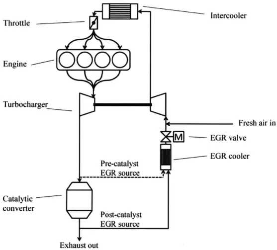
drawn from either of these two locations as shown in figure 1.1.

Pre-catalyst exhaust has gases like C0

, SO, and NO, which have the potential to dissolve in

the condensate, making it acidic and corrosive. The NOx gets reduced to nitrogen gas and

some ammonia in the three-way catalytic converter. So, when post-catalyst exhaust gases

condense, the condensate formed is near-neutral to slightly basic, which is significantly less

corrosive. This has meant that the EGR flow in engines with cooled LP EGR has usually

been taken post-catalyst.

Intercooler

[000

0]

Figure 1.1: Schematic of Exhaust Gas Recirculation system in an engine, showing EGR cooler and pre- and post- catalyst EGR sources

However, Roth et al.J2 1 showed that using pre-catalyst gases for EGR might give fuel economy benefits. Firstly, lesser exhaust flows through the catalyst, which means there is a smaller pressure drop across it. The resultant larger pressure drop across the turbine is beneficial. The LP EGR can also be driven more easily since the extraction point pre-catalyst is at a higher pressure than a post-catalyst point. Further, some of the products of incomplete combustion (hydrocarbons, H2 and CO) are not oxidized in the catalyst and are instead

channeled back to the combustion chamber. Here, they may release their energy by getting completely oxidized, as well as improve combustion characteristics. These factors together gave a reported BSFC improvement of 1.5 - 3.5 % by using pre-catalyst EGR over post-catalyst.

I

Since the formation of corrosive, acidic condensate in the EGR cooler is considered as the

limiting consideration while choosing between pre- and post-catalyst EGR, this motivates a

study of this condensate. This project is an attempt to address the question of what gases

contribute to the acidity of the condensate, as well as to get experimental data about the

condensate under different engine running conditions.

1.2 Background and Literature Review

There has been a historic interest in the formation of acids in the exhaust system of engines

[3,4,.

_{In the past, when the level of sulfur in the fuel was high, up to 0.03% by weight, studies}

showed that the SO

formed during combustion would get converted to SO

in the oxidation

catalyst. As the exhaust cooled, the hygroscopic SO

would combine with water to form

sulfuric acid. This would be present in the exhaust as particulate matter in the form of small

droplets. It led to corrosion, but more importantly widespread air pollution, acid rain and

posed a health hazard.

The advent of three-way catalytic converters has necessitated the reduction of gasoline sulfur

to increasingly lower levels as SO

is an inhibitor of its performance. EPA's Tier 2 Gasoline

Sulfur program has required the average level of sulfur to be lower than 30ppm by weight

since 2004, which was a 90% reduction from previous levels

Beginning in 2017, EPA's

Tier 3 Gasoline Sulfur standards will come into effect, which will further limit the sulfur

content to an annual average of 1 Oppm

Whereas sulfuric acid dominated the composition of the exhaust condensate formed

previously, it is expected that the lower sulfur levels would decrease or eliminate the sulfuric

acid in the condensate.

A detailed study by Hunter'

_{into the exhaust condensate composition for various catalyst}

types of the time was reported in 1983. Here, the condensate composition and pH were tested

for various engines, oxidation and/or three-way catalysts, fuels and air-fuel ratios. Ion

chromatography was used to measure the anion concentrations in condensates, whereas pH

was measured by an Orion pH meter. Acidic condensates were formed in the case where

there was no catalyst (which can be interpreted as pre-catalyst condensate) or there was an

oxidation catalyst. These mainly had the anions sulfate, nitrate, chloride (where the origin of

chloride ions was from chlorine in the fuel) and some nitrite. Almost no

carbonate/bicarbonate was present in the highly acidic samples, but was present in the near

neutral ones. In systems which had only a three-way catalyst, it formed near neutral to basic condensate on account of the ammonia in the gas. There was no systematic difference reported between using gasoline or gasohol/E10 fuel (gasoline mixed with 10% ethanol by volume).

Data of the acidic condensates from this report was used to gauge the predictability of pH from the anion concentrations. By charge neutrality between the condensate's anions and cations, and the definition of pH,

[H-]=2.[S04 ]+[Cl-]+[NO-]+[NO(] (1.1)

pH = loglo[H ] (1.2)

These equations are used to give the predicted (calculated) pH of a sample based on the anion concentrations. This was done for the acidic samples, using the anion data presented in the report, and plotted against the reported (measured) pH values.

6

Figure 1.2: Comparison of reported sample pH with pH calculated from reported anion concentrations using charge neutrality. Only acidic samples were selected because they are

The majority of the points lie close to the line where calculated pH equals the measured

value. The two points on the far right of the figure are for exhaust condensate formed

downstream of a three-way catalyst converter. There is some ammonia dissolved in the

condensate which reduces the hydrogen ion concentration predicted by equation 1.1, raising

its actual pH above the predicted value.

This exercise gives the following results:

* If the anion concentrations of a condensate sample are known, by measurement or by

theoretical calculations, its pH can be predicted.

* For condensates formed from early 1980s engine and catalyst technology using

high-sulfur fuel, the main anions that determined the pH were sulfates, nitrates and nitrites

(in the case of highly acidic samples).

* Carbonates/bicarbonates may be present in near neutral samples.

* Chloride anions can be neglected in laboratory conditions if the fuel contains no

chlorine. This is because other sources of chloride, i.e. sea salt near coastlines and

rock salt on the road used to melt snow in winters are also absent in the laboratory.

Thus, the exhaust gases selected for pH prediction in the current report are

C02

, SOx and

NOx.

1.3 Research Objectives

The main objective of this study is to identify the cause(s) of the acidity of pre-catalyst

exhaust condensate, in relevance to current engine and fuel technology.

This is done in two steps:

0 Relate the exhaust gas composition to the fuel and engine operating condition. Then

relate the pre-catalyst exhaust condensate's composition and pH to the composition of

the exhaust gas from which it is formed. Combine these, to characterize the

condensate properties based on operating conditions. This was done theoretically,

with the assumption that gas and condensate are in equilibrium. The calculations are

presented in Chapter 4.

a Experimentally observe the dependence of pre-catalyst condensate's pH on the engine

operating condition to validate the proposed theory. For this, the engine's load,

air-fuel ratios and spark timing were varied to get different exhaust gas compositions.

The results of these experiments and comparisons with the predicted pH are presented

in Chapter

5.

Thus, an understanding of the pre-catalyst condensate's properties will help to judge the

feasibility of pre-catalyst cooled LP EGR.

Chapter 2: Experimental Setup

0000

-0

Figure 2.1: Schematic of Experimental Setup showing sampling point in exhaust system, NO2 measurement apparatus and condensate collection apparatus with vacuum pumps

Figure 2.1 shows the layout of the system used to measure exhaust gas NOx and NO2 concentrations and to collect the condensate. The primary path of the exhaust gas originating in the engine is through the turbine and catalytic converter to the test cell's exhaust trench, which takes the gases away safely. Downstream of the turbocharger, there is a NOx-cum-lambda sensor. The sampling port for NO2 measurement and condensate collection is at the same location. All tubing and fittings starting from this sampling port are made of Type 316 Stainless Steel or chemically resistant plastic PVDF to prevent corrosion. This also prevents contamination of the sampled exhaust with any metal ions that may have dissolved in the condensate formed on tube walls during warm up, had the tubes been made of less resistant materials. (Initial experiments done when copper tubes were used led to non-repeatable

results.) The tubing is also insulated so that once the exhaust gas warms it up, it remains

warm even when exhaust gas flow is stopped.

From the sampling port, the exhaust gas goes to a three-way valve. One path takes it to the

NO

sensor through a can of desiccant. The NO

sensor requires that the gas sample be below

50*C and non-condensing. The warm, insulated tubing before the desiccant ensures that there

is no condensation, thus no loss of NO

through dissolution. After the desiccant, the

non-insulated tubing allows the gas to cool and enter the sensor. Here, the gas is drawn safely into

the wide-mouth of a funnel and through a vacuum pump to the exhaust trench. The other path

takes the exhaust gas to the condensate collection system, which is described in detail below.

In this path, there is a port for the injection of bottled NO

gas into the sampled exhaust, so

that the effect of additional NO

on the condensate can be studied.

2.1 Engine

A General Motors Ecotec 2.0 LNF engine was used in the experiments. Introduced in 2007, it

was part of Generation II of the Ecotec family. It is an inline 4-cylinder, turbocharged, direct

injection engine with compression ratio 9.2:1 and displacement 1998 cubic centimeters,

giving a maximum power of 260 hp (190 kW) at 5300 rpm.

An eddy-current type dynamometer was used to absorb the engine power and a dynamometer

controller maintained constant speed.

2.2 Fuel Used

All the engine tests were carried out with Haltermann HF0437 fuel, which is an EPA Tier II

Emission Certification gasoline. Several batches of fuel were used over the tests, with

stoichiometric air/fuel ratio varying from 14.5 to 14.6, and RON from 96 to 97. The sulfur

concentration varied between 27 ppm and 33 ppm by weight. The test reports of these batches

are attached in the appendix B.

2.3 Condensate Collection Apparatus

Exhaust gas was drawn from the sampling port by a vacuum pump through a heat exchanger

(condenser) and flask to form and collect condensate samples. The rotary vane vacuum pump

was rated for a maximum flow rate of 10 cfm (4.72 L/s) at open flow. The high flow rate

through the condensate collection system was a sizeable fraction of the total exhaust flow coming from the engine: and it enabled relatively rapid collection of condensate.

A Volkswagen EGR cooler (Part number 03G-131-512-AD, from the 2006 Jetta TDI) was used as the heat exchanger for condensing the exhaust gas. This shell-and-tube heat exchanger has two pathways for gas flow within its body: the first one has thin channels for gas to flow surrounded by the coolant and provides maximum cooling; the second one has one large channel as a bypass and provides little cooling. The in-built valve was kept open to the first pathway only. The liquid coolant to the heat exchanger was municipal water. Its temperature varied according to the season, between 50C and 200C. While a real engine EGR cooler uses engine coolant at a temperature of 80 - 1000C. the municipal water provided higher cooling for faster condensate formation.

As the exhaust would pass through the condenser at a high flow rate. the condensed water would get entrained in the flow in the form of droplets. To ensure that these droplets would collect in the flask rather than get drawn into the vacuum pump, an appropriate inlet adapter was used. The gas entered the adapter through the side and hit the inside wall. where the condensate would form larger drops that could flow into the large flask. The inlet to the vacuum take-off (where the gas exited) was situated in the middle of the flask. well below the point of entry. so that the entrained droplets would not flow directly with the gas into the take-off and had a chance to coalesce.

Exhaust drawn to vacuum pump

Inlet adapter

(shown with grey

outline) Cold exhaust

from condenser

-carrying droplets

Tapered ground glass

oint with thin layer of

Drops coalesce on oil to make it air-tight

sides of adapter and flask and

collect in the flask

~-large

NOT To SCALE

2.4 Sensors

The NOx level was measured using a Horiba MEXA-720 NOx analyzer. This has a non-sampling type zirconia solid-state sensor that simultaneously measures NOx and oxygen in the exhaust stream. The analyzer converts the oxygen concentration to give an output for the air-fuel equivalence ratio (lambda).

NO2 concentration was measured using a GasAlert NO2 detector (from BW Technologies by Honeywell). This is also a solid-state sensor, over which gas below 500C must flow in a non-condensing state. Its least count is 0.1 ppm, which has an important implication since the exhaust NO2 concentration was found to be below 0.1 ppm in some cases (discussed in

section 4.3). The measuring range is 0 - 100 ppm, and it was calibrated using 50.4 ppm NO2 gas in balance nitrogen.

The collected condensate samples were poured from the flask to small beakers. Here, their pH was measured by a VWR sympHony B lOP pH meter, which requires samples of at least

Chapter 3: Experimental Procedure

3.1 Preparation

The setup was prepared for running and collection of data with the following steps:

* Refuel the engine's fuel tank.

" Remove the pH sensor from its storage fluid, clean it with deionized water and

calibrate with buffers of pH 7, 4 and 10 (in that order). Clean the condensate

collection flask and beakers with deionized water too.

* Check if desiccant (in the NO

measurement line) is fresh. Change if it is exhausted.

* Calibrate NO

sensor in fresh air for zero measurement and with 50 ppm NO

gas for

span measurement.

" Check water pressure from the municipal supply after filtration (that supplies water

for cooling of dynamometer, engine's intercooler and condensate collection system).

If the pressure is too low, change the water filter to a new one so that the pressure

drop in it decreases.

The pH sensor was calibrated each day measurements were taken. The NO

sensor was

initially calibrated once in 20 days. This was fine for higher NO

levels as the span

calibration did not change in that period. But later it was noticed that once exposed to high

NO

concentrations, the sensor would not go back to zero even in fresh air. After this, the

zero reading was checked in fresh air after every run, and recalibrated if needed.

3.2 Data Collection

The following steps were performed for measuring exhaust gas and condensate properties for

each operating point:

* Switch on the engine with nominal running parameters: 1200 rpm, stoichiometric

air-fuel ratio, nominal spark timing and low load (throttle 18% open). Let it run with

these parameters till engine coolant warms up to 80*C.

" Set engine operating point. If it is the first run of the day, this is at 1500 rpm with

other parameters same as the above. Otherwise, air-fuel equivalence ratio, spark

timing and load are varied in accordance with the lambda sweep / spark sweep

experiment. These parameters are kept constant until the CA50 and GIMEP reach a

steady value. (CA50 is the crank angle for

50%

heat release for a combustion cycle).

* Switch on vacuum pump to draw exhaust through the three-way valve and tubes of

the sampling system for NO

measurement at a high flow rate to warm them up.

These insulated tubes then remain warm so that there is no condensation within them

later when NO

is measured with very low exhaust flow rates.

* Note the NOx concentration. Connect the flow cap on the NO

sensor and note its

reading.

* Switch three-way valve to pass exhaust to the condensate collection system. Turn on

vacuum pump to start condensate collection.

* Discard first few milliliters of collected condensate from the flask. It takes around

5

minutes of running for this, as condensate starts flowing down from the walls of the

condenser only after some of it is built up.

* Collect about 15 mL of condensate in the flask, which takes 10

-

20 minutes

depending on the operating point; then turn off the three-way valve. Switch off

engine; then measure the condensate pH along with its temperature.

* Disconnect tubing for condenser. Pass deionized water through it to wash off the

condensate film on its walls. Then blow hot air through it to evaporate all the water.

The engine operation across all runs is with nominal valve timing according to the production

calibration and closed loop lambda control by the ECU. This lambda control has oscillations

at around 1 Hz about the set value, so that at stoichiometric setting, the air-fuel ratio is

alternating between rich and lean.

The first 'standard' run, which is the same every time experiments are done, is used to

measure the NO, NO

and pH values to see if they match with the corresponding readings on

previous days. Usually, these were relatively consistent. If not, the cause of change was found

and fixed. For example, this could be an air leak into the condensate collection system, at the

ground glass interface between flask and adapter.

The measures to maintain steady state are so that the pH readings are more repeatable. This is

why measurement is taken after the engine operating point becomes steady. It is also the

reason why the initially formed condensate is discarded: after this the condenser reaches its

own steady state.

The condenser is cleaned and dried after every run so that condensate from the previous

operating point does not remain sticking to its walls and affect the pH of the current run.

This, too, is to improve repeatability of pH data.

The condensate temperature was between

25

C

and 33

C, depending on ambient conditions.

Thus, 30'C was used as the condensate and gas temperatures for theoretical calculations.

Chapter 4: Theoretical Calculations

In this chapter, the contributions of individual exhaust gas components to the pH - or hydrogen ion concentration - of the condensate is determined as a function of the engine operating conditions. The assumptions for the calculations are shown below:

Gases Exhaust

Condensate

Dissolved gases ;Acid < H+ + Anion

Figure 4.1: The equilibria relating various species in the exhaust gas and condensate. Blue arrow indicates phase equilibrium, red arrows indicate chemical equilibrium.

The gases considered are CO2, SO, and NO,. These flow continuously over the condensate which collects. Physical equilibrium between the gases and condensate means that they are at the same temperature and their concentrations in the two media are related by Henry's Law. Then, the equilibrium constants of the chemical reactions leading to formation and dissociation of the acids relate the various concentrations within the condensate.

It is important to emphasize that the exhaust gas components themselves are not in chemical equilibrium at the low temperatures of condensation. The products of combustion are in equilibrium at high temperature when they are formed. But as the gases cool down during expansion in the cylinder, their composition gets 'frozen' due to slow chemical kinetics compared to their residence time in the exhaust system. It is this frozen composition that dissolves in the condensate and participates in acid formation.

4.1 Contribution of CO2

CO2 is produced by burning of gasoline, a hydrocarbon fuel, according to the following idealized reactions. For rich combustion (A < I):

C'H8 7 + /4+1

)(O

)

I

c ~3*d

0.8 - 1) is (4.1) which means the CO concentration is approximately thrice that of hydrogen. Using this fourth equation, the four unknown values a. b, c and d. are calculated.

( CO,

a

a+ b c d+2 ( + I 17X3.773)

(4.2)

gives the mole fraction of CO2 in the gas. Similarly. for lean combustion (A> 1).

CH 87 +2(1 + 87XO

+3.773N)->

)(3.773N2)

0

1 + + '+(- !)( 7)

+)J(1+

X3.773)

(4.3)

Thus, the CO2 mole fraction is known as a ftinction of lambda:

0.16 -- _ - -- -0.14 0.12 0.08 0.06 0.04 0.02 0 0.8 0.85 0.9 0.95 1 1.05 1.1 1.15 1.2 Lambda

Figure 4.2: CO2 concentration as a function of air-fuel equivalence ratio

27 4-0 X a 0 E 0 U xco :::

Once this is known, Henry's Law gives the concentration of dissolved CO

in the condensate

as follows:

Pco2 = XCQ * P (4.4)

gives the partial pressure of CO

, where p is the total pressure. In the exhaust system, it is

very nearly 1 atm.

XCO2 = Pco2 *VC02 /

HcO2

gives the mole fraction of CO

in water, where <bcO2 is its fugacity coefficient (unity at the

low pressures here) and Hco

is the Henry's Law constant. The value of Hco

at 30

C is

calculated to be 183.8 MPa from a correlation by Carrol et al.

The mole fraction of dissolved CO

is converted into molarity (moles/L) as:

[C02 (aq)]

= nC0_ n

PS-

nC2

V m

n

+n

Here, nco2 moles of dissolved CO

in a solution of volume V are considered. The density and

average molar weight of the solution is considered approximately the same as the density and

molar weight of water.

Dissolved CO

reacts with water to form carbonic acid, which then dissociates. The overall

reaction is:

C0

KaCO2(a>

[H2](H

-

/kg

K

The first dissociation constant value shown is at 30

C, using data by Read,

. HCO3 is a very

weak acid and does not further dissociate a second time to C032-. By charge neutrality,

[H+ ] = [HCO3 ] (4.8)

Thus, [H4+] is calculated from equations 4.7 and 4.8. In this case the hydrogen ion

concentration is expressible explicitly as:

This is plotted as a function of lambda. It can be seen that the predicted pH is nearly constant at a level near 4.5. 0 0 U 0 CL 7 6 5 4 3 2 1 1E-7 1E-6 0 1E-5 .9 C 1E-4 0 0 1E-3 r 0 1E-2 1E-1 0.8 0.85 0.9 0.95 1 1.05 1.1 1.15 1.2 Lambda *

Figure 4.3: Calculated contribution of CO2 to condensate pH

I

combustion phasing is changed from early to late in the cycle (by retarding the spark timing). the exhaust gas temperature increases. This means there is higher post-oxidation of unburnt hydrocarbons and CO in the exhaust stream leading to a corresponding increase in CO2 level.

But this change is small compared to the change in CO2 by varying air-fuel ratio, and has a

negligible effect on pH.

4.2 Contribution of SO,

The gasoline available in the market, and that used in the experiments here, has about 30 ppm of sulfur by weight. Another source of sulfur is the lubrication oil that gets into the combustion chamber. All this sulfur gets oxidized to mainly SO2 in the engine, and other minor species such as SO3, H-2S, COS and CS2 .

29

Firstly, the relative contribution of sulfur from the fuel and lubrication oil is compared.

For the engine in the experimental setup, fuel economy is taken to be 22 mpg, i.e. fuel is consumed at the rate of 1 gallon per 22 miles. The experiment gasoline density is 0.742 kg/L. Thus, the sulfur content in the exhaust is calculated per mile as follows:

1 gal

L

kg 30 kg

Exhaust S from fuel= x 3.78 x 0.742 - = 3.82 mg /mile

22 mile gal L 106 kg

(4.10)

Oil consumption in the engine is taken to be a typical value: 1 quart (0.25 gallons) per 10000 miles. The oil density and sulfur concentration for a sample of the oil used in the test setup engine were tested to be 0.855 kg/L and 1953 ppm by weight. Thus,

Exhaust S from oil = 0.25 gal x 3.78 xO.855 x 1953 kg =0.16 mg /mile

10000 mile gal

L

(4.11)

Hence, the lubrication oil is found to be a minor contributor of sulfur in the exhaust gas due to its low consumption, despite its higher sulfur content. But it adds about 5% more sulfur in the exhaust stream. For further calculations, fuel sulfur is taken to be 32 ppm by weight to include this.

Given the low level of sulfur in the fuel compared to previous studies, the next step is to find out if sulfur oxides S02 and S03 still contribute significantly to the hydrogen ion contribution of the condensate formed. For this the concentrations of these gases in the exhaust gas are found from the total sulfur concentration.

A study by Kramlich et al.1101 on the chemistry of sulfur oxidation in hydrocarbon combustion measured the distribution of the sulfur among the various sulfurous product species. According to it, S02 was the dominant product in both rich and lean flames. The following data is taken from the study:

" At a slightly rich point (X = 0.8), approximately 4-6% of the sulfur appeared as H2S

(depending on the hydrocarbon fuel), and less than 0.5% as CS2 and COS each. The rest, i.e. 94% on an average, was SO2.

" _{At stoichiometric combustion, the only significant sulfurous species were SO2 and}

SO3, with SO3 making up only 0.6% of the total sulfur.

I

M S02 - SO3 '4-100 98 96 94 92 90 0.8 1 1.2 Lambda

Figure 4.4: Distribution of fuel sulfur as SO, in the exhaust. Adapted from Kramlich et al. 1

These results were reported to be independent of the sulfur dopant in the used were H2S. SO2 and C4H4S (thiophene).

fuel. The dopants

This distribution of sulfur in exhaust SO2 and S03 is used to calculate their concentrations. knowing that fuel sulfur is 32 _{ppmn. For a given mass of the fuel burnt.}

"'nyhaus,=nI 'fl

(A

The mass of the exhaust as well as its sulfur content is known. The mass fractions of the SO2 and SO3 thus obtained from the data above are converted to mole fractions _{Xs02 and xs03.} shown in figure 4.5.

As in the case of CO2. the partial pressure of SO₂ can be calculated and used with Henry's Law constant, HS0 2 = 1.038 M/atm, to get the dissolved SO2 concentration:

Ps = xso, * P (4.13)

[,O2(aq)]= p,,, * H ,,() (4.1 4)

-- S2 3 2.5 ...

2

0

6

Figure 4.5: SO, and SO3 concentrations as functions of equivalence ratio

The dissolved SO- forms sulfurous acid, which dissociates twice according to the following reactions: SO,(aq)+H,0<-> H +HSO 3 KH]HQ- _{0.0 123 mole / kg} [S(-, (aq)] HSO ++H +SO (4.15) [H+][SO 2 ] [HSO, 6.5* I0-'nmole / kg

The values of the Henry's Law constant and dissociation constants are calculated at 300_C from the method by Goldberg and Parker.

S03 _{is present in the exhaust gas only in the order of 0.01 ppm. But unlike SO2, it is very} soluble and practically goes completely into the condensate. That is, its Henry's Law constant

0.5

0

Ku?' (aq) (4.16)

is infinite1

_{. Here, it reacts with water to form sulfuric acid. This too dissociates twice as}

shown:

(4.17)

The first dissociation is complete and the second dissociation's equilibrium constant is taken from Marshall and Jones '31. Thus, the SO3 that goes into solution exists as the bisulfate and sulfate species. Their total concentration can be calculated by using the total condensate and SO3 formed per unit mole of fuel burnt.

[HSOJ ]+[SO42- ]- n, _ ms * fraction aSO M.W-s (4.18)

H4

VM condensed _{H 2O,conden el}

Here, ms is the mass of sulfur per mole of fuel, i.e. 32*106 * 13.87 g, fraction as SO3 is taken

from figure 4.4, and the method of calculating the volume of condensate is explained in appendix A.

By charge neutrality,

[H] =[HSO]

+2.[SO

]+

Equations 4.14 - 4.19 are solved for the 6 unknown quantities. Knowing the hydrogen ion concentration gives the pH, which is plotted in figure 4.6. The pH is seen to be nearly constant at 3.8. Also, the determined concentrations of the anions show that SO2 concentration is the deciding factor for the pH. Bisulfite (HSO3-) is the dominant species at rich operation, but sulfate (S042-) becomes equally important at the lean case. This shows that pH is very sensitive to SO3; it is only the extremely low concentration that keeps it from

dominating the acid formation.

When the combustion phasing is varied instead, the cylinder peak temperature and exhaust gas temperature change. The SOx concentration data from Kramlich et al.110' was collected at temperatures of 1500K to 1800K. They report a temperature dependence for the rate of oxidation of fuel sulfur, but the final concentrations of the sulfur product gases did not

change. Thus, there is no effect of combustion phasing change on the SO, contribution to the condensate pH. 7 1E-7 0 6

1E-6

MS

Figure 4.6: Calculated contribution of SO, and SO3 to condensate pi

4.3 Contribution of NO,

At the high temperatures at which the burnt gases in a cylinder are present. some of the nitrogen and oxygen molecules break down into their atomic form. These react to form mainly NO, and some NO2, which are together called NOx. As the temperature decreases during the expansion stroke and in the exhaust system, the reactions get 'frozen' and the NO, gases' concentration stay well above their equilibrium values for exhaust temperatures. Hilliard and Wheeler1 4 1 studied the formation and concentration of NO2 in gasoline and diesel engines. They found that it increased with load, up to about 60 ppm at full load. Because these levels were much higher than the equilibrium between NO, 02 and NO, would suggest, they suggest that NO reacts with 0, OH or O2 H during the expansion stroke to form NO, and the reaction then gets frozen.

On the other hand, Lenner et al.11 16] suggest that NO reacts with 02 to form NO, in the exhaust system where the temperature is between 200 - 300"C. They found that during

engine idling, the NO2/NO, ratio may go up to 30%, much higher than the expected 2%. This was for a car with air injection into the exhaust stream.

In the current study. NO and NO2 concentrations were directly measured in the test setup at different engine loads for the calculation of pH contribution of NO, gases. These were done prior to condensation. For NO2, which was measured after passing the gas through a desiccant, the concentration was converted from dry to wet before plotting.

+ NO, 10 bar -. 0- NO, 5 bar ,='- N02, 10 bar - N02, 5 bar

3000 - - 30 E E 0. 0. . 2500 25 3 2 2000 - 20 2

.E

.S

E

Figure 4.7: Measured NO and NO2 concentrations as functions of equivalence ratio and load at 1500 rpm. The 10 bar GIMEP values are for 13" aTDC CA50. the 5 bar GIMEP values are

for 8 " aTDC CA50.

For both the load cases shown in figure 4.7. as combustion goes from rich to stoichiometric, the NO formation rises steeply. whereas the NO2 concentration remains near zero. Moving further to lean combustion, the NO curve flattens out and the NO2 starts to increase steeply. The measured NO2/NO, ratio is approximately I % for the leanest cases and less than that for all others. This ratio is almost identical as a function of lambda for the two cases, as shown in figure 4.8.

- 10 bar ... 5 bar 1.2 1- -0 z0. 6 -0.4 0.2 0 0.8 0.85 0.9 0.95 1 1.05 1.1 1.15 1.2 Lambda

Figure 4.8: NOJ/NOX for different loads at 1500 rpm. The 10 bar GIMEP values are for I3" aTDC CA50, the 5 bar GIMEP values are for 8 aTDC CA50.

In figure 4.7, the NO2 concentration measured for the 5 bar plot was 0.0 ppm for the rich cases, which means the value was below the instrument sensitivity of 0.1 ppm. The NO, measurements for the 10 bar rich running cases are in fact erroneous: it was seen that after exposing the NO2 sensor to high levels of the gas, it does not show a zero reading even for fresh air. So, these values should be zero just like the 5 bar case.

The same measurements were made as a function of combustion phasing. The spark timing sweep was started at Knock Limited Spark Advance (KLSA) and then retarded by 5 crank angle degrees for every data point. The results were plotted as a function of the CA50 in figure 4.9. With retarded combustion, the peak gas temperature is low resulting in lower NO, formation. It is seen that NO2 falls off faster than NO on retarding combustion, i.e. NO2/NO, goes from close to 1% at advanced spark to <0.5% at retarded values.

NO N02 1200 --- 12 E E CL CL

o

0

_z

Figure 4.9: Measured NO and NO2 concentrations as functions of combustion phasing at 1500 rpm. 3 bar GIMEP and A = I

Now that the NO and NO2 concentrations for various operating conditions are known. the pH can be predicted for these. These gases react in the gas phase to form nitrous and nitric acids, which then dissolve and dissociate in the condensate. Simultaneously. the gases dissolve in the condensate where they react in the liquid phase too. There is also some dimerization of the NO2, which is considered negligible here. These reactions and the complex mixed-phase equilibria were studied by Schwartz and White[1 7 1 to give a set of consistent reaction properties. The following two overall reactions for the formation of nitrate and nitrite are chosen (labeled as in their study):

NO(g)+ N),(g)+ H O " > 2H+ + 2NOi [M2]

[H+] -'( 101M

Km = ] 2.27*10 M4

/atmr (4.20)

3N0(g)I+ H2O< >2H+ + 2NO- + NO(g) [M3]

[ g)+H][N[M]1

These equilibrium constants were adjusted for 30C using the van 't Hoff equation:

=~~e H > In =H -I1 L (4.22)

dT RT 2

Ke (To) RTO T

where To = 298.15 K and R is the universal gas constant. The standard enthalpy change

values, AH0, and Keq(To) values were taken from Schwartz and White's data.

NO2 is much more soluble and reactive than CO2 and SO2. Unlike them, enough of NO2 dissolves into the condensate that its equilibrium concentration is significantly lower than its initial value. Thus, the approach of using Henry's Law with the initial gas concentration does not work with NO₂.

On the other hand, it is not as soluble as SO3, which goes completely into the condensate.

Thus, the approach of the reaction reaching completion cannot be used either.

Instead, the more basic method of conserving the moles of reactants consumed and products formed is used. The initial mole fractions of NO and NO2 are the measured values prior to

condensation. For every mole of fuel burnt, the amount of exhaust gas is known (Appendix equations A.2 and A.5). Thus,

No. of moles of NO initially = xNO * nexhaus; formed

No. of moles of NO2 initially = xNO2 * nexhausformed (4.23)

Suppose reaction M2 moves in the forward direction by y moles and M3 by z moles. Then,

No.of moles of NO finally = xNO nexhausformed - Y + Z

No.of moles of NO2 finally = xNO2 nexhausformed - y - 3z (4.24)

Thus, the equilibrium partial pressures of the two gases are given by:

PNO XNO * nexhaus formed Y + Z p (4.25) nexhaus4 remaining

SXNO2 nexhaus;Iormed - y - 3z

nexhausremaining (4.26)

where the nexhaust,remaining is from equation A.10.

Thus, the anion concentrations are [NO, ]= v VII .i() nd c [N0] 2z VH ).conidensed (4.27) (4.28)

where the VfIo 0condensed is from equation A.9.

Finally, by charge neutrality.

[H] [NO] +[NOj] (4.29)

The equations 4.20 - 4.21 and 4.25 - 4.29 are used to solve for the seven variables (equilibrium partial pressures of two gases. condensate concentrations of three species. x and y). This gives the pH contribution of NO, gases. The values corresponding to the measurements in figure 4.7 are shown here:

-- 10 bar -- 0- 5 bar 7 6 5 . . . . _ _ _ _- _ -. _ -- -__ 4 2 . . . . 1 1E-7 1E-6 0 1E-5 . 1E-4 0 (U C 1E-3 -0 0 1E-2 _E 1E-1 . 0.8 0.85 0.9 0.95 1 1.05 1.1 1.15 1.2 Lambda

Figure 4.10: Calculated contribution of NO and NO2 to condensate pH as a function of equivalence ratio and load

For the two load cases. the pH is very acidic in the lean region where the NO, concentration is high. At rich operation points. the pH is nearly neutral.

39

I

ox

z

For the rich running region, there is uncertainty in predicting the pH because the NO2 concentration is not known exactly. It is between 0 and 0.1 ppm, but the pH is very sensitive to NO2 such that it can lie anywhere in the shaded region. The lower bound was determined by taking the NO2 concentration to be 0.0 1 ppm for A = 0.8 and 0.05 ppm for A = 0.9. The values for the 10 bar plot are shown in this region as more acidic (pH ~ 3.5), as the measured but incorrect NO2 level used for them was 0.5 - 2 ppm. It can be seen how varying NO2 concentration from 0 ppm to 2 ppm changes the pH from neutral to ~-3, which is quite acidic. The predicted pH plot with combustion phasing, corresponding to the data in figure 4.9 is:

7 - -- - - - 1E-7 o 6 1E-6 Z 0' 0 z --.0 5 1E-5 4 1 E-4 0 3 1E-3 0 2 - 1E-2 a.. ---- -- 1E-1 -10 0 10 20 30 40 CA50 (* aTDC)

Figure 4.1 1: Calculated contribution of NO and NO, to condensate pH as a function of comnbustion phasing at X = 1, 3 bar GIMEP

Again, the pH is more acidic at advanced combustion due to the higher levels of NO, formed. In these calculations, it was seen that nitrate was the predominant anion with much less nitrite. Also, the pH was mainly determined by the NO, concentration and nearly independent of the NO level. This is because both reactions M2 and M-3 are driven forward to produce more acid if NO, levels rise, but an increase in NO concentration drives one reaction forward and the other backward.

4.4 Combined Equilibrium pH from All Gases

The hydrogen ion contributions of each of the gases can be combined by including all the anions in the charge neutrality equation.

[H] [HCO; ] +[HS, ] + 2.[S0 + [ HS4 ] + 2.[SO> ] + [NO] + [N( ]I (4.30)

These concentrations are calculated by the simultaneous solution of all three sets of equations from the three previous sections, while replacing the individual charge balance equations in them by equation 4.30. This gives the combined total pH trend.

E 1.. -a 0 0-7 6 5 1E-7 1E-6 0 'Z: 1E-5 1E-3 1E-2 >. M 1 1E-1 0.8 0.85 0.9 0.95 1 1.05 1.1 1.15 1.2 Lambda

Figure 4.12: Calculated condensate pH at equilibrium due to all gases at

5 bar GIMEP, 8 " aTDC CA50 as a function of equivalence ratio.

The individual contributions of the gases towards the formation of hydrogen ions are shown in figure 4.13 a. (The vertical scale in this graph is reversed compared to figure 4.12). It is evident that at rich operating points, the pH is determined by SO,. Here, the SO3/SO, fraction is low anyway. so SO2 concentration determines pH. From stoichiometric to lean operating points, NO, is the maJor contributor to pH. NO and NO2 react together to form acidic condensate. but the pH is much more sensitive to NO2 concentrations.

3

1E-2 M NOx 0 1E-4 C O 0 1E-7 1E-6 C0 o 1E-5 0.8 0.9 1 1.1 1.2 Lambda

1E-2

Figure 4.13: a. Contribution of dissolving gases to form hydrogen ions in condensate, and b. Anion composition of the condensate, as functions of equivalence ratio

Figure 4.13 b shows the individual anion concentrations which add tip to equal the hydrogen ions' charge (as in equation 4.30) in decreasing order from top to bottom. Nitrate ions are the highest. except at rich conditions. Sulfur appears as bisulfite at rich conditions and sulfate and bisulfate at lean conditions.

The effect of combustion phasing at stoichimetric operation on the calculated shown below. 7 6 5 4 3 2 1 combined pH is --- -- 1E-7 1E-6 0 1E-5 ., 1E-4 ₀ 2 1E-3 0 1E-2 -1E-1 -10 0 10 --20 30 40 CA5O (0 aTDC)

Figure 4.14: Calculated condensate pH at equilibrium due to all gases at 3 bar GIMEP. A = I as a function of combustion phasing.

Since the deciding factor for pH at stoichimetric operation is NO,, this curve follows the predicted pH due to NO, only (from figure 4.11) very closely. It is very slightly more acidic than the values there, taking into account the smaller contributions from SO, and CO2. At advanced CA50 points, where the NO, is at the highest. there is no difference between the two curves. The NO, levels have a relatively lower influence at retarded combustion cases, but the difference between the two plots is still just 0.1 pH point here. This decreasing influence is shown in the condensate composition graphs of figure 4.15.

E

-o

0* 0