Control and reliability of optical networks in multiprocessors

(1)

Control and Reliability of Optical Networks in

Multiprocessors

by

James Jonathan Olsen

S.B., Massachusetts Institute of Technology (1981) S.M., Massachusetts Institute of Technology (1985)

Submitted to the Department of Electrical Engineering and Computer Science in partial fulfillment of the requirements for the degree of

Doctor of Philosophy at the

MASSACHUSETTS INSTITUTE OF TECHNOLOGY May 1993

@

Author ... ...

Department o Electri c\Engineering and Computer Science April 30, 1993

Certified by ... Agarwal

Anant Agarwal

Associate Professor of Computer Science heCkeis Supervisor

A ccepted by ... ... ./.. ... .. .... ... dommttee Campbell L. Searle

-Chair ,epartmental Committee on Graduate Students

[JUL 15 1994

(2)

Control and Reliability of Optical Networks in Multiprocessors by

James Jonathan Olsen

Submitted to the Department of Electrical Engineering and Computer Science on April 30, 1993, in partial fulfillment of the

requirements for the degree of Doctor of Philosophy

Abstract

Optical communication links have great potential to improve the performance of interconnec-tion networks within large parallel multiprocessors, but the problems of semiconductor laser drive control and reliability inhibit their wide use. These problems have been solved in the telecommunications context, but the telecommunications solutions, based on a small number of links, are often too bulky, complex, power-hungry, and expensive to be feasible for use in a multiprocessor network with thousands of optical links.

The main problems with the telecommunications approaches are that they are, by definition, designed for long-distance communication and therefore deal with communications links in isolation, instead of in an overall systems context. By taking a system-level approach to solving the laser reliability problem in a multiprocessor, and by exploiting the short-distance nature of the links, one can achieve small, simple, low-power, and inexpensive solutions, practical for implementation in the thousands of optical links that might be used in a multiprocessor.

Through modeling and experimentation, I demonstrate that such system-level solutions exist, and are feasible for use in a multiprocessor network. I divide semiconductor laser reliability problems into two classes: transient errors and hard failures, and develop solutions to each type of problem in the context of a large multiprocessor.

I find that for transient errors, the computer system would require a very low bit-error-rate (BER), such as 10-23, if no provision were made for error control. Optical links cannot achieve

such rates directly, but I find that a much more reasonable link-level BER (such as 10- 7) would

be acceptable with simple error detection coding. I then propose a feedback system that will enable lasers to achieve these error levels even when laser threshold current varies. Instead of telecommunications techniques, which require laser output power monitors, I describe a software-based feedback system using BER levels for laser drive control. I demonstrate, via a BER-based laser drive control experiment, that this method is feasible. It maintains a BER of

10-9: much better than my error control coding system would need. The feedback system can

also compensate for optical medium degradation, and can help control hard failures by tracking laser wearout trends.

For hard failures, a common telecommunications solution is to provide redundant spare optical links to replace failed ones. Unfortunately, this involves the inclusion of many extra, otherwise unneeded optical links, most of which will remain unused throughout the system lifetime. I present a new approach, which I call 'bandwidth fallback', which allows continued use of partially-failed channels while still accepting full-width data inputs. This provides, at a very small performance penalty, a high reliability level while needing no spare links at all.

I conclude that the drive control and reliability problems of semiconductor lasers do not bar their use in large scale multiprocessors, since inexpensive system-level solutions to them are possible.

Thesis Supervisor: Anant Agarwal

(3)

Acknowledgements

I would also like to thank Anant, my thesis supervisor, for his assistance and guidance in shaping my research program. I am grateful to my readers, Bob Kennedy and Tom Goblick, for their valuable advice. My thanks also go to the many other people at Lincoln Lab and LCS who provided me advice and assistance. I would like to thank my wife Batya for her support and encouragement in this work.

This work was sponsored by the Department of the Air Force under contract F19628-90-C-0002.

(4)

(5)

3.1 Data Communication vs. Telecommunication 3.2 Data Communication Hardware ... 3.3 Optical Sources ... 3.3.1 Optical Modulators ... 3.4 Optical receivers ... 3.5 Transmission Media ... 3.5.1 Free Space ... 3.5.2 Holographic Networks ... 3.5.3 Planar Waveguides ... 13 .. .. .. ... .. .. ... ... . . ... . .. . 14 .. .. .. ... .. .. ... ... . . ... . .. . 15 20 20 20 21 22 22

(6)

3.5.4 Fiber Optics ... . ... 30

3.5.5 Assumptions of the analysis ... ... 31

3.6 Optical Switching and Computing ... . . . . . ... . 31

3.6.1 Optical Switching ... 31

3.6.2 Optical Computing ... 32

3.7 Multiprocessor Networks ... ... 32

3.7.1 Mesh Networks ... 33

3.7.2 Hierarchical Networks ... 33

3.7.3 Butterfly-type networks ... ... .34

4 Optical data link reliability problems 35 4.1 Transient errors ... ... 35

4.1.1 Assumptions of the Analysis ... .. 38

4.2 Hard Failure ... ... .. . . 38

4.2.1 Gradual wearout ... 39

4.2.2 Random failure ... 42

4.3 Hard Failure Probability ... ... 43

4.3.1 Gradual wearout probability . ... ... .. 43

4.3.2 Random Failure Probability ... ... 44

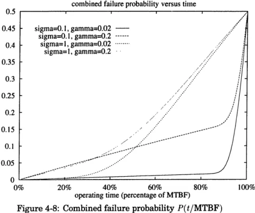
4.3.3 Combined failure probability ... .. 45

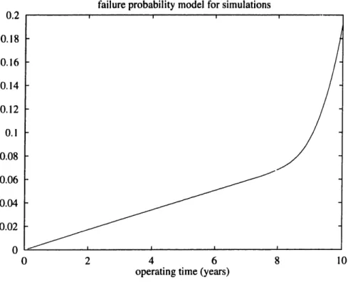
4.3.4 Probability model for analysis ... .. 46

4.3.5 Assumptions of the Analysis ... .. . .. 48

4.4 Sum m ary ... ... 48

5 Prototype network 49 5.1 Optical channels ... .. ... 49

5.2 Network Nodes ... 52

5.3 Prototype network operation ... ... 53

6 Error Control Coding 57 6.1 Acceptable error levels ... 57

(7)

6.2 Coding Theory ...

6.2.1 Error detection vs. Error correction . . . . 6.2.2 Error-detection coding ...

6.2.3 Error-Detection Coding system implementation 6.3 Error Diagnosis ...

6.3.1 Transient Error Diagnosis ... . .

6.3.2 Hard Failure Diagnosis . . . . 6.4 Summ ary ...

7 Intelligent Laser Drive Control

7.1 The Laser Drive Problem . . . . 7.2 Conventional Solutions ...

7.2.1 Fixed laser drive . . . . 7.2.2 Analog-feedback laser drive control . . . . 7.2.3 Very-low-threshold lasers ...

7.3 Intelligent laser drive control ... 7.4 Laser drive control experiments ...

7.4.1 Experimental Setup . . . . 7.4.2 Feedback Program ...

7.4.3 Temperature experiments ... 7.4.4 Optical loss experiments ... 7.4.5 Feedback Reduction Order ... 7.4.6 Bias-Only Drive Control ...

7.4.7 Digital-to-Analog Converter Implementation . . 7.4.8 Feedback Stability . . . . 7.4.9 Achievable error-rates . . . . 7.5 Benefits of Intelligent Laser Drive ...

7.5.1 Unbalanced data transmission . . . . 7.5.2 Laser Lifetime Monitoring ...

7.6 System Implementation ... 7.7 Summary ... 58 58 61 63 64 64 65 65 66 66 68 69 70 71 72 72 74 77 79 81 84 84 88 89 90 90 92 93 : : : : : : : :

(8)

8 Redundant Sparing 95

8.1 Acceptable failure levels ... .... ... 95

8.2 Redundant Sparing ... 96

8.3 Redundant channel switch ... ... 96

8.3.1 Single-stage substitution switch theory ... 99

8.3.2 Multi-stage substitution switch theory. ... 103

8.3.3 Substitution switch implementation ... 105

8.4 Redundant sparing lifetime ... . . ... ... . . . 106

8.5 Sum m ary ... 108

9 Bandwidth Fallback 109 9.1 Detour Routing ... 109

9.2 Bandwidth Fallback Concepts ... . . .. .. ... .. . 111

9.2.1 Basic Operation ... ... 111

9.2.2 Interaction with substitution switches ... 114

9.3 Bandwidth Fallback Simulations ... .... 116

9.4 Conclusions ... 117

10 Conclusions 119 10.1 Results of the research ... 119

10.2 Topics for further study ... 120

10.3 Feasibility of Optical Multiprocessor Networks ... 122

A Laser Drive Control Experimental Setup 123 A.1 H ardw are ... 123

A.1.1 Laser/Driver Board ... 123

A.1.2 Photodiode/receiver board ... .... 125

A.1.3 Computer Interface ... ... 129

A.1.4 Data Link Analysis Board ... 129

A .2 Softw are ... .. ... ... ... ... .. ... ... ... ... . 133

(9)

List of Figures

2-1 Communication energy vs. Distance (based on [1, 21)

3-1 Free-Space Communication with Compound Optics 3-2 Free-Space Communication with Holograms . . . . . 3-3 Communication via Planar Waveguide ...

3-4 Subnetwork interconnection via optical fiber ...

3-5 Dual Electronic/Photonic Interconnection Network .

4-1 Optical communication error model . . . .

4-2 Error rate vs. Signal-to-noise ratio... 4-3 Component failure rate vs. time . . . .

4-4 Log-normal probability distributions . .

4-5 Laser wearout vs. time...

4-6 Laser wearout probability P,(t/T,) . .

4-7 Random failure probability Pr(t/Tr) . .

4-8 Combined failure probability P(t/MTBF)

4-9 Simulation failure probability model . .

5-1 Prototype multiprocessor network . . . . . 5-2 Prototype optical link ...

5-3 Mesh routing example ... 5-4 Mesh routing deadlock ...

6-1 Linear block code generation and checking

7-1 Semiconductor laser output power vs. drive current

7-2 Semiconductor laser driver circuit . . . .

23 28 29 29 30 34 . . . . . 36 . . . . . 37 . . . . . 39 . . . . . 40 .. ... . .. .. .. .. . 41 . . . . . 44 . . . . . 45 . . . . . 46 . . . . . 47 . . . . . 50 ... .. .. . .. .. .. . 50 ... ... . . ... . ... 54 .. . ... . . ... .. .. 55 . . . . . 61 67 . . . . . 6 8

(10)

7-3 Fixed laser drive ...

7-4 Analog-feedback laser drive control . . . . 7-5 Intelligent laser drive control . . . . 7-6 Intelligent laser drive experimental setup . . . . 7-7 Photograph of Laser Drive Control Experimental Setup 7-8 Laser Drive Control software state diagram . . . . 7-9 Laser Drive Control over temperature ... . .

7-10 Laser Drive Control with optical loss ...

7-11 Feedback Reduction Order (temperature experiment) . . 7-12 Feedback Reduction Order (optical loss experiment) . . .

7-13 Bias-only Feedback (temperature experiment) ... 7-14 Bias-only Feedback (optical loss experiment) . . . . 7-15 Laser control effectiveness vs. DAC precision . . . .

Substitution switch example ...

Substitution for one failed link . . . . Two-stage substitution switch ...

Substitution for three failed links ...

Four-stage substitution switch . . . . Substitution for 15 failed links . . . . Substitution switch algorithm examples ... Failure pair mapping ...

Second-level substitution algorithm examples Laser failure timescale transformation . . . . Spares/channel m vs. median system lifetime tm .

. . . . . 97 . . . . . 98 . . . . . 98 . . . . . 99 . . . . . 100 . . . . 101 . . . . . 102 ... 103 . . . . . 104 . . . . 107 . . . . . 108 Virtual Channels ... Detour Routing Example ... Bandwidth fallback switch ... Switch configuration for various fractions of bandwidth . Substitution switch with bandwidth fallback ... Performance vs. time with 5 spares/channel ... Performance vs. time with 10 spares/channel ... S. 110 S. 110 . . 112 . . 113 S. 115 S. 116 . . 117 69 70 71 73 75 76 78 80 82 83 85 86 88 8-1 8-2 8-3 8-4 8-5 8-6 8-7 8-8 8-9 8-10 8-11 9-1 9-2 9-3 9-4 9-5 9-6 9-7

(11)

9-8 Bandwidth Fallback performance with no spares ... 118

A-1 Photograph of Laser/Driver Board, front view ... 124

A-2 Photograph of Laser/Driver Board, rear view ... 126

A-3 Simplified Laser/Driver board Schematic ... 127

A-4 Photograph of Photodiode/receiver Board ... 128

A-5 Photograph of Computer Interface ... ... 130

A-6 Computer Interface Schematic (analog section) ... 131

(12)

List of Tables

6.1 Error-detection code characteristics ... . . . . .. . . 63 7.1 4b5b line code ... 91 9.1 Data transmission through a 75%-bandwidth channel ... .. . 114

(13)

Chapter 1 Overview

For many years, the promise of massively parallel computing (combining large num-bers of inexpensive processors into powerful systems) has beckoned computer archi-tects. This promise is now being fulfilled, and it is apparent that the interconnection network between processors is one of the primary factors determining the overall performance of a multiprocessor system. The important parameters governing inter-connection network cost and performance include inter-connection density, bandwidth, and reliability.

Recent advances in optical technology suggest that optical interconnect networks will soon be viable for use in multiprocessors. Optical networks offer the potential of vastly increased bandwidth and connection density, compared with electrical networks. Currently, the most widely used paradigm for optical data communication relies on semiconductor lasers as optical sources. Such lasers present a number of reliability problems. In the telecommunications context, where such optical communications find increasingly wide use, these problems have already been solved.

However, telecom solutions, based on a relatively small number of long-distance links, are often ill-suited to a multiprocessor network containing thousands of short-distance links. In this thesis, I investigate reliability solutions which are more appro-priate to the multiprocessor context.

(14)

1.1 The Reliability Problems

The use of optical communication networks in multiprocessors poses two main relia-bility questions.

1. Multiprocessor systems are exceedingly intolerant of data transmission error.

How can the optical links achieve a sufficiently low data error rate?

2. Semiconductor laser failure data, when extrapolated to systems with large num-bers of lasers, suggest that overall reliability of such a system might be unac-ceptably low; does this mean that semiconductor lasers are impractical for use in large-scale multiprocessors?

Telecommunications links intended for telephone use are often designed to achieve Bit-Error-Rates (BER) on the order of 10- 9 or 10-12, with the best systems achieving values around 10-15 [3]. However, data communications within multiprocessors will require much better BER levels to assure reliable operation, such as 10-23 for example.

(A 10-23 rate would be needed in a 4096-channel system with 64-bit 1-Gword/sec

channels, if one allowed 0.1 error/year.) Optical device research continues to seek lower BER levels, but the extremely low levels required on multiprocessor applications will almost certainly remain elusive on raw channels without error coding.

Another aspect of semiconductor laser operation is relevant to both transient-error and hard-failure performance: laser threshold current variation. As a laser ages, it wears out and eventually fails. This wearout manifests itself as an increase in laser threshold current[4], and the laser drive must provide sufficient current to compensate for the increased threshold. Threshold current also increases with laser temperature. Increased threshold, with fixed drive, will result in lower laser output and higher error rates. Also, high-speed lasers must be driven with a bias current approximately equal to the threshold, and an old (or hot) laser therefore 'fails' if the drive circuit does not supply sufficient bias current to compensate for the increased threshold.

Semiconductor laser reliability is constantly improving, but it is still potentially a limiting item for system reliability. For example, a high-reliability laser might have an MTBF (Mean or Median Time Between Failure) specification of 100,000 hours. A 1024-node multiprocessor might employ 300,000 lasers; linear extrapolation of the

(15)

failure rate would lead one to conclude that such a system would have an MTBF around 20 minutes: a completely unacceptable level of reliability. (Some researchers have gone so far as to conclude that this renders semiconductor lasers unsuitable for use in large-scale multiprocessor networks, and have instead pursued other optical sources, such as light modulators pumped by a central, high-power gas laser [5].)

Laser failures can be divided into two broad categories: wearout failures and random failures. While random failure times follow an exponential distribution, that is, they can be modeled as arrivals of a Poisson process, wearout failure times follow a log-normal distribution [4]. Therefore the simple linear extrapolation used above:

Component MTBF Number of Components

is valid only with respect to random failures, but not with respect to wearout failures, since a set of n identical Poisson processes of rate A is equivalent to one Poisson process of rate nA, but such a relation does not apply to a process with log-normally distributed arrival times.

Nevertheless, the true system MTBF will still likely be inadequate without special provision for recovery from laser failure. For example, even if we have a random-failure laser MTBF of 10,000,000 hours, the system MTBF due to random random-failure in a 300,000 laser system will be about 30 hours, which is still unsatisfactory. As the system ages, wearout failures will also come into play, further increasing the failure rate.

1.2 Reliability Solutions

My solution to the laser reliability problem has three major parts:

* Control transient errors by Error Detection Coding, and retransmission on error, * Control laser drive current with an intelligent software-based feedback loop based

on the observed Bit Error Rate (BER), and

* Control of hard failures with 'Bandwidth Fallback', which provides the reliabil-ity benefits of large-scale redundant sparing, without the expense of providing spares.

(16)

1.2.1 Error Detection Coding

It is apparent that some form of error control coding scheme will be required to solve the bit-error-rate problem. Error control coding strategies can be placed in two broad categories: Forward Error Correction (also called error-correction coding), in which enough redundant data are included in each transmission to re-derive the original data in spite of one or more transmission errors, and Automatic Retransmission Request, in which only enough redundant information is sent to enable the detection of errors, and the sender is asked to retransmit any data received in error.

Data storage systems, such as magnetic disks, are generally constrained to use Forward Error Correction, since it is impossible to ask for a retransmission of data if it has been corrupted on the storage medium. Similarly, high-speed telecommunication systems will use Forward Error Correction because retransmission, while theoretically possible, would be impractical due to very long transmission delays (relative to bit transmission times).

By contrast, the sender and receiver in a multiprocessor system are relatively close, and Automatic Retransmission Request is quite feasible. [An exception to this would be multiprocessors which are constrained to operate in pre-set instruction se-quence, such as Single-Instruction, Multiple-Data (SIMD) systems, since the times when retransmission is required can, of course, not be determined ahead of time.] A retransmission strategy, combined with a very simple error-detection coding scheme, allows the use of data links with dramatically relaxed error rate requirements.

1.2.2 Intelligent Laser Drive Control

High-speed operation of most semiconductor lasers usually requires the adjustment of the laser drive current level as the laser threshold current varies with age and temperature. Design for long-term reliable operation of an optical network requires that the problem of laser drive level control be addressed.

The standard solution to this problem in a telecommunications context is to im-plement a laser light output power monitor, and to use this to form a feedback loop controlling the laser drive level (I illustrate this in Figure 7-4). This is an excellent approach for telecom applications, where the size, optical complexity, and expense of

(17)

such a feedback loop is easily absorbed in an already large and expensive support system for each laser.

The multiprocessor context is different. When one considers the use of dozens of lasers on each channel, and many thousands of lasers in each system, the complexity and size of each laser link becomes much more important. Implementation of a laser light monitor system in a multiprocessor network would entail an oppressive hardware overhead, and would be much more difficult to justify than in the telecommunications context.

Fortunately, we can exploit the coding approach described in the previous section, and the error-rate flexibility it allows, to suggest an alternative approach: intelligent (i.e., software-based) laser drive feedback control using the data-link error rate as the feedback control variable. The error rate is, in fact, the data-link parameter that we ultimately wish to control. Light-monitor-based approaches control the laser light output level for feedback only as an easily-accessible and controllable (at link level) surrogate for the error rate.

Given the Automatic Retransmission Request error-control system outlined above, one may implement an intelligent laser drive control system with the addition of one or two very simple Digital-to-Analog converters per laser (or set of lasers), easily implemented en masse in an integrated circuit. The Digital-to-Analog converters are controlled by the sending processor, which adjusts the drive level based on how frequently its neighbors request retransmission of data.

1.2.3 Bandwidth Fallback

From even the cursory analysis I have given above in Section 1.1, it is clear that some provision must be made for continued system operation after laser failure occurs. Even if the intelligent drive control system could completely eliminate the wearout problem (not a very likely prospect), we would still have to handle random failures. In telecommunications, a common approach to failure problems is to provide redundant spares, to be used in place of failed links. I examine how the provision of redundant spare optical links could be implemented in a multiprocessor network, and show that this would be an adequate approach to the hard-failure problem if one could afford the cost of providing enough spare links.

(18)

I then examine two approaches to eliminate this cost: use of time-shared alternative paths to replace failed channels, and providing for variable-width data transmission to exploit whatever remaining data width is available (which I call 'bandwidth fall-back'). Bandwidth fallback is an idea for efficient use of the remaining bandwidth in a partially-failed channel. With the addition of one multiplexer and one register per bit, the channel can be made usable at certain fractions of its full bandwidth, of the form 1/2, 3/4, 7/8, 15/16, etc. It can provide almost the same performance as large-scale redundant sparing, without needing any spares. (Bandwidth Fallback is also applicable to electrical networks, given off-board connections are generally much less reliable than on-board or on-chip connections.)

1.3 Summary of Results

As long as one avoids the type of inflexible system design that precludes the use of Automatic Retransmission Request error controll, an optical multiprocessor network need only implement coding for error detection, as opposed to both detection and cor-rection. With this approach, we demonstrate that a very simple linear error-detection code can to achieve the needed level of error control with minimal overhead: relaxing the optical-link BER requirement from 10-23 to 10- 7_.

Given such a coding scheme, laser drive control can be accomplished without the need for light output power monitoring and the associated analog feedback loops, by using the link's bit-error-rate to control the laser drive level. I have designed and implemented a software-based laser drive control system for an experimental free-space optical data link. I have conducted experiments on the drive control system over varying temperatures, showing excellent control of error-rate. (Incidentally, it controls the laser output level quite well without the use of a light level monitor!) I show that a 5-bit Digital-to-Analog converter would be adequate for level control in this experimental setup, and that the experimental feedback system is stable, with a gain margin of at least 10 dB. Additional experiments demonstrate recovery from optical medium degradation: a capability not possessed by traditional monitor-based control schemes. i also explain how an intelligent laser drive control system can help

(19)

deal with laser wearout failures by facilitating long-term monitoring of laser wearout trends.

I find that providing redundant spare lasers (if one could afford enough of them) would result in acceptable system reliability. I show that, with only a small per-formance penalty, the implementation of alternative routing and bandwidth fallback can provide the same reliability benefits, without the spares. Alternatively, they can provide the same performance as redundant sparing, with a great reduction in the number of spares needed.

In the final section, I offer suggestions for further research on this topic, and conclude that the laser reliability problem can, in fact, be solved by proper use of system-level reliability solutions.

(20)

Chapter 2 Why Optics?

Why would one want to use optical interconnect in a multiprocessor? Studies of mul-tiprocessor optical interconnect have cited many advantages of optical over electronic interconnect [6, 5, 7, 8]. The major advantages are outlined below.

2.1 Connection Density

From a network theory perspective, the most interesting advantage of optical inter-connect is its potential for increased inter-connection density. This is due to the contrasting natures of the electron and the photon.

Electrons are fermions and carry a charge; they therefore interact strongly with each other, both due to electromagnetic effects and due to the Pauli exclusion principle. Photons are bosons and electrically neutral; they interact weakly, if at all. Because of this, multiple light beams can cross the same point in space without interfering, while multiple wires cannot. This property of optical interconnect may render some previous analyses of multiprocessor networks, which implicitly assumed connection density limits, inapplicable.

2.2 Bandwidth

One of the most immediate benefits of optical interconnect is increased bandwidth. While electrical network interconnects have been pushed to 1 Gbit/second [9], it be-comes increasingly cumbersome as frequency components progress higher into the

(21)

microwave spectrum. Optical links now in use for telecommunications achieve 3.4 Gbit/second data rates over distances of 50 km [1]. Laser modulation rates of 15 GHz have been reported [10].

Fundamentally, an optical link is a modem (modulator-demodulator), with an opti-cal carrier signal. Phenomenal bandwidth potential is not surprising, since the carrier being modulated typically has a frequency of 200 THzi or more. The bandwidth avail-able on an optical link is not limited by the link itself, rather by the electronic circuits on either end. Progress in Opto-Electronic Integrated Circuits (OEIC's) suggests that the highest-speed electronic signals associated with the link will need to extend no further than a single chip (or chip module). This implies that serialization (multiplex-ing) of the electrical signals will be needed in order to exploit the full bandwidth of the optical link.

Data rates in conventional electronic signaling (that is, baseband signaling) are limited by dispersion effects, due to the very broad bandwidth relative to the center frequency. Optical telecommunications links also suffer from dispersion, but over the relatively short distances encountered within multiprocessor interconnection networks

(< 1 km), dispersion is very small.

2.3 Fanout

Electronic logic signals have traditionally supported high fanout (that is, multidrop) connections. Conventional bus architectures (for example, VMEbus or NuBus) rely on electronic fanout to broadcast signals among all the boards on the bus.

Unfortunately, the multidrop model breaks down at high switching speed, due to transmission line reflections. As Knight points out [11], while it is theoretically possible to adjust and tune the transmission line to produce a matched multidrop line, in practice it is so cumbersome as to be impractical. Practical high-speed (> 1 Gbit/sec) electrical interconnect will generally be point-to-point.

Optical interconnect poses no such restriction. Multidrop connections are perfectly feasible, limited only by the total transmitted power available. A fundamental ques-tion, to be answered by further research, is how best to exploit this capability, or

(22)

whether it is worth exploiting.

2.4 EMI Immunity

Unlike electrical signals, optical signals are virtually immune to electromagnetic in-terference (EMI) and similar effects, such as ground-loop noise. This is an important practical advantage, as anyone who has constructed large-scale high-speed computing systems can attest. Although quite valuable, this electromagnetic interference immu-nity does not appear to have a direct impact on the choice of a particular computer architecture. Instead, makes implementation of any large-scale system more practical.

2.5 Communication Energy

Power dissipation is an important factor in all high-speed computing systems, and a large part of the power is dissipated in communication, not in calculation [12]. Miller

[2] argues that, fundamentally, optical communication requires less energy than does electrical communication, over all but the shortest distances.

Miller's argument is based on the characteristic impedance of free space, Zo = 377. All practical transmission lines will have a characteristic impadance much less than

Zo, since the impedance depends only logarithmically on the line's dimensions. (At one

conference [13], Miller put it: "All transmission lines are 50 Ohms." A bit of hyperbole, but not far from the truth.) We can see this illustrated by the impedance formula for a vacuum-filled coaxial line: Z = Zo ln(r2/r1). Even to get the impedance up to Z0,

the outer conductor would have to be 500 times larger than the inner conductor, and any dielectric material would make it even more difficult.

Small electronic devices can pass only small currents, and are therefore high-impedance devices, poorly matched to driving transmission lines. Traditionally, large buffer amplifiers (pad drivers) are placed between the logic elements on a chip and the transmission lines off-chip. Since the transmission line must be properly terminated (somewhere), the low-impedance drivers use up considerable power in charging and discharging the line. Low-impedance drive is also the source of current-switching transient (dl/dt) noise: a major design constraint.

(23)

1-'1 , " 1"

200

20 Iling

Phi

R

Line Length (microns)

Figure 2-1: Communication energy vs. Distance (based on [1, 2])

Optical signaling avoids the free-space impedance problem, since it operates on quantum mechanical (photons-electrons) rather than classical physical principals. Photodiodes are already well matched to logic inputs, and multiple-quantum-well techniques may produce low-threshold lasers and/or optical modulators which can be driven directly by microelectronic gates.

It now seems that optical signaling is the best approach for long-distance com-munications, and electronic signaling is the best approach for communication over microscopic distances. Ross [1] (probably relying on Miller's work [2]), offers a graph like the one in Figure 2-1 to argue that optical communication is preferable to electri-cal communication over distances longer than some critielectri-cal length. The exact value of this critical length depends on the specific parameters of the links being compared, but Ross puts it at 200m. (This is based on fundamental energy considerations. If, instead, one used present-day economic considerations, one might find the the critical length to be closer to 200cm, or even 200m.)

If energy is the ultimate limitation, it seems that optics may eventually supplant electronics for all interconnect above the intra-chip level. It does so now for commu-nications over long enough distances, and the criterion for 'long enough' will certainly grow shorter and shorter as optical technolh-gy progresses.

(24)

Chapter 3 Multiprocessor optical networks

Optical interconnect is an active research field, and the state of the art is advancing rapidly. Here I describe the state of the art as it applies to optical networks for multiprocessors.

3.1 Data Communication vs. Telecommunication

Driven by the telecommunications market, optical communication hardware is now

highly developed and continues to improve. Telecom hardware now achieves

phe-nomenal performance, such as fibers with 0.1 dB/km attenuation, and 3.4 Gbit/sec links with 50-km distances between repeaters [1]. Current research topics, such as

soliton-based signaling [14], promise even more impressive results.

Unfortunately, this superb telecommunications hardware is not directly applicable to multiprocessor networks, since it is designed to satisfy different constraints. In tele-com, long-distance performance is the key, since this governs the number of repeaters required on a link, and repeaters form a major part of the cost of a link. Also, telecom size and power constraints (per link) are often less stringent than the corresponding constraints for con. :uter hardware.

Because of this, telecom optical links tend to make the cost-performance tradeoff in favor of high performance and high cost per link: too high a cost for use in parallel processor networks, which need many, many links. (We need many links in order to increase bandwidth without increasing electrical switching speed, and to reduce the latency inherent in serializing the data for transmission. Such latency is no problem

(25)

in telecom systems, since it is overwhelmed by the speed-of-light transmission delay.) Optical datacom (that is, short-distance communication) hardware is well behind the leading edge of performance. For example, the Fiber Distributed Data Interface (FDDI) local-area network [15] is only now coming into wide use, and it uses a signaling rate of 125 Mbit/sec: over 25 times slower than the fastest telecom links.

Given the differing cost constraints, it seems likely that datacom hardware perfor-mance will remain well behind the state of the art in telecom. However, this state of the art is advancing so rapidly that we can reasonably expect optical datacom hardware to achieve current telecom performance within a few years.

3.2 Data Communication Hardware

While there are many possible implementations of a fixed optical communication link, they share some common features. A link consists of an optical source, an optical receiver, and a transmission medium.

3.3 Optical Sources

The two major optical sources for communication links are light-emitting diodes (LED's) and semiconductor lasers. Another option is the use of optical modulators acting on an externally generated laser beam.

Light-Emitting Diodes

Light-emitting diodes are very simple devices, and have a number of advantages for use in an interconnect network: they are cheap, easy to fabricate, and reliable. In some moderate-performance applications, light-emitting diodes are the perfect choice. For example, FDDI [16] uses them as optical sources.

Unfortunately, the light-emitting diode has limited bandwidth. Light-emitting diodes are quite capable of signaling rates around 100 Mbit/sec (as in FDDI), and with some effort can be made to switch at 1 GHz, but at higher switching rates they become increasingly impractical. For >1 Gbit/sec rates, lasers or optical modulators appear to be the most reasonable sources.

(26)

Semiconductor Lasers

The most straightforward laser light source is the semiconductor laser, with its drive current modulated by the desired data stream. Modulation of semiconductor lasers at 15 GHz has been demonstrated, and it seems safe to say that the laser switching rate will likely be limited by the drive electronics before it is limited by the laser itself

Microfabrication of surface-emitting semiconductor laser arrays is showing impressive results, such as densities of 200,000,000 lasers/cm2 _{[1], and threshold currents around}

1 mA (potentially much lower [171).

Semiconductor lasers have a number of problems, but probably the most diffi-cult one for this application is laser reliability. Laser reliability figures are hard to come by, and depend on several factors, but the current state of the art is on the or-der of 105 or 106 hours MTBF. For a massively parallel processor with thousands of lasers, laser failure will be a fairly common event, and must be handled P -acefully. A semiconductor-laser-based system will likely have to cope with the laser reliability problem by providing considerable fault-tolerance in the higher-level design.

3.3.1 Optical Modulators

To avoid the semiconductor laser reliability problem, an alternative approach using optical modulators has been proposed [5]. In this scheme, large, high-power external lasers are used to provide an optical 'power supply' which is routed to the inputs of op-tical modulators. The external laser can be made quite reliable and wavelength-stable. The modulator outputs produce a modulated light beam similar to that otherwise pro-duced by the semiconductor laser. The modulators and lasers have broadly similar characteristics; in fact, multiple-quantum-well modulator arrays (see Section 3.6.1) are almost identical to multiple-quantum-well laser arrays, omitting the laser mirror on one side.

Modulator-based schemes have their own problems, chief among them the need for optical power distribution. However, a number of groups (notably Honeywell) are convinced of their superiority, especially in systems subject to wide temperature variations, such as military systems.

(27)

appar-ent. A significant factor in deciding the issue will be the extent to which it is practical to handle the laser reliability problem with inexpensive, system-level solutions.

3.4 Optical receivers

Optical receivers are relatively straightforward. The optical signal illuminates a diode, causing a photoelectric current. This is then amplified to the desired logic levels (or used directly [181).

Either PIN (p-intrinsic-n) or avalanche diodes may be used. The avalanche diode produces a stronger signal, but is more difficult to fabricate. Either diode may be fabricated in silicon, but at the high data rates of interest here, III-V materials such as GaAs are also of interest.

This thesis assumes the use of suitable photodiodes, with high-speed amplifiers on the same chip or module, if needed.

3.5 Transmission Media

Optical transmission media are another important concern in optical network research, since the medium partly determines the topological and other constraints on the optical network.

3.5.1 Free Space

The simplest medium is free space. The pure free-space link (a light source shining directly on a receiver) is finding applications now, over short distances such as those in inter-board communication. While pure free-space links are interesting, some other free-space approaches are potentially more useful in computer networks. A number of these alternatives involve free-space links with some reflective or refractive device between source and receiver.

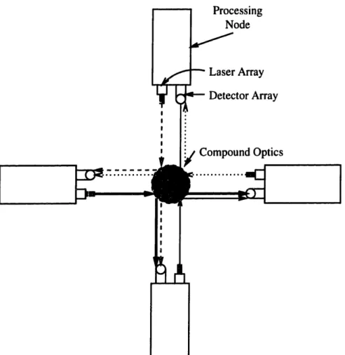
Free-space communication schemes (and holographic schemes, to some extent) offer the opportunity to exploit the ability, mentioned in Section 2.1, of optical signals to cross in the same point in space. This is a significant advantage, but it is not without cost. All free-space approaches require extremely accurate mechanical alignment,

(28)

Laser Array Detector Array

Figure 3-1: Free-Space Communication with Compound Optics

posing problems for manufacturing and, more particularly, for repair. (Re-alignment of a replacement component in the field may be quite difficult.) Some form of adaptive alignment would be a significant advantage.

Considerable research has dealt with the use of compound optics as a means of distributing light from source to receiver (see Figure 3-1). This generally imposes a constraint of 'space-invariance' on the transmission pattern: the output pattern (relative to the input beam) must be the same from all ports.

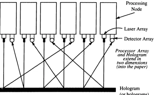
3.5.2 Holographic Networks

Holographic interconnect is another form of free-space link, with the optical distribu-tion device being a hologram [191 (see Figure 3-2). Holograms do not impose a space-invariance constraint. The pattern reflected by the hologram is basically arbitrary, within certain angular constraints. These angular constraints can be significantly

(29)

I

(or holograms) Figure 3-2: Free-Space Communication with Holograms

,% essing ode Array tor Array

i~l~l

aliliil n V avegUle

(extends in two dimensions)

Figure 3-3: Communication via Planar Waveguide

relaxed by employing multi-layer holograms (that is, several holograms sandwiched

together).

3.5.3 Planar Waveguides

Oversimplifying, one might say that a planar waveguide [20] is a 'printed-circuit board' for optical signals (see Figure 3-3). It offers connections between arbitrary points in a plane, with crossovers, combiners, and splitters available. Being self-contained, it obviates most of the alignment problems of free-space approaches such as holograms. Unfortunately, their transmission efficiency is still quite low, currently around 0.3 dB/cm. (Compare this to 0.1 dB/km for high-quality fiber!)

:ssing ode Array tor Array Array gram Sin nsions gaper) m I

(30)

Figure 3-4: Subnetwork interconnection via optical fiber

Planar waveguides offer moderate connectivity with moderate implementation dif-ficulty. They appear to be a possible compromise between point-to-point fiber connec-tions (easily implemented, but low connectivity) and holograms (difficult implementa-tion problems, but very dense connectivity). Lin [21] suggests an interesting combined hologram/waveguide approach.

3.5.4 Fiber Optics

Optical fiber is by far the most highly developed optical medium today. Optical fiber is now produced which imposes only a few dB of loss over a distance of hundreds of kilometers. Unfortunately, such long-distance performance is of little relevance to multiprocessor networks, where distances will be less than ten meters.

The basic disadvantage of fiber is that it is implemented on an individual link basis, one fiber at a time. Progress is being made on the use of fiber bundles: parallel groups of fibers terminated together [22], but it is still premature at this time to consider a large-scale multiprocessor with interconnections solely based on fiber bundles.

However, fiber does have one important advantage: flexible geometry. All of the previously-mentioned optical media require the communicating nodes to be aligned in a pre-determined geometry, and fixed in that alignment. Optical fibers, on the other hand, offer flexibility in two senses: mechanical flexibility, allowing communica-tion between points which are not in rigid alignment, and design flexibility, allowing arbitrary placement of the two endpoints of the fiber.

Fiber bundles might therefore be of considerable usefulness in connecting optical subnetworks which were implemented by other, less flexible means. The subnetworks could be made as large as practical, and then used to create a still larger network via fiber connections. The Figure 3-4 illustrates this idea.

(31)

3.5.5 Assumptions of the analysis

Since the laser reliability questions are substantially the same for all the optical media presented here, my analysis need not assume the use of any particular medium. However, the analysis of transient errors in Section 4.1 is particularly important for the less power-efficient media, such as planar waveguides, since the importance of the power vs. error-rate tradeoff is magnified in those cases.

3.6 Optical Switching and Computing

A potentially strong motivation for the use of optical networks is optical switching and computing. There is no intrinsic distinction between optical switching and optical computing: any reasonably efficient switching system can be made to do computation. However, while 'optical switching' means what it says, the term 'optical computing' has had the special connotation of purely optical computing. [To confuse matters further, the meaning of 'optical computing', at least in some quarters, seems to be evolving toward 'optical communication between electronic logic devices': just the sort of thing I examine in this thesis. I shall use the older meaning.]

3.6.1 Optical Switching

Optical switching has been studied for some time, and optical switches for telecom have been well developed. However, switches for massively parallel systems must be extremely fast and compact. Presently-available switches are generally interferometer designs (such as Mach-Zehnder) which tend to be large, or liquid-crystal designs which tend to be slow. Current research into newer designs, such as Bell Lab's work on multiple-quantum-well (MQW) devices [171, is quite interesting for this application.

Multiple-quantum-well switches might serve as the modulators for the external-laser design mentioned in Section 3.3.1. The external-external-laser design tends to blur the dichotomy between Optical Communication and Optical Switching set forth above.

(32)

3.6.2 Optical Computing

One might consider optical computing to be the Holy Grail of this field. All of the electro-optical approaches are highly mismatched in speed, with the electrical portion as the speed-limiting factor. If true optical computing could be achieved, it might improve computer performance by orders of magnitude.

True optical gates have been demonstrated [23], but they involve high power lev-els, and are not fully restoring. Pure optical gates are far from practical computing implementation for the time being, and seemingly for the near future as well.

Reflecting this discouraging prospect, the term 'optical computing' is apparently evolving toward a different meaning: electronic computing with purely optical inter-connection. (In a sense, this is what the purely optical gates do as well, since their optical non-linearity is fundamentally based on electronic interactions.) Bell Labs re-searchers vigorously assert that their self-electrooptic devices (SEED's) [24] implement 'optical computing'.

Self-electrooptic devices, and other 'optical computing' devices in the new sense of the term, while remarkable devices, are fundamentally electronic logic gates with optical input and output, and therefore limited by electronic switching speeds.

While high-speed optical communication hardware is practical now and is in wide use, high-speed (that is, high reconfiguration speed) optical switching hardware is less advanced, and optical computing hardware (in the original sense) will not be practical for some time, if ever. Therefore, the analysis in this thesis treats the reliability of optical communication only. Analysis of optical switching and computing is an area for further research.

3.7 Multiprocessor Networks

Multiprocessor networks have been a fertile subject of research for over two decades, and continue to be so. A vast literature is available on various interconnection schemes. However, no consensus has been reached as to which approaches are optimal, even in the extensively-studied electronic regime, much less in the optical regime.

(33)

Nevertheless, some interesting mathematical results on performance limits of var-ious networks have been achieved (for example, Dally's work on mesh networks 1251). Many of these analyses assume that network bisection bandwidth is the limiting fac-tor. The assumption may be true for electronic interconnect (although even this is disputed), but is unlikely to be valid for optical networks. On the other hand, the analysis of Agarwal [261 would seem to be applicable to optical networks, in the case where he assumes a limit on node size instead of network bandwidth.

3.7.1 Mesh Networks

Mesh networks, also called grid or nearest-neighbor networks, possess an elegant simplicity. The basic idea is to place nodes in a plane (or a volume) in a regular pattern, and form a communication network by linking each node with its nearest neighbors. Their short communication lengths and point-to-point links make mesh networks especially well-suited to electronic implementation, negating a number of the advantages mentioned in Section 2.

An optical mesh network may still be worthwhile. As noted in Section 3.5.1, point-to-point free-space interconnect is well advanced, and is now close to practical imple-mentation. This could be used to implement an optical mesh network. The existing research into electronic mesh networks should be directly applicable, with the optical links looking like very-high-speed wires.

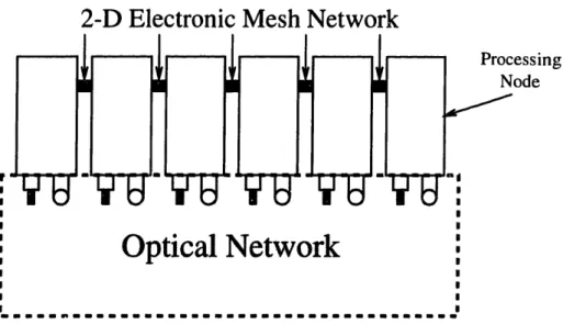
If the optical mesh network is not used, a very interesting possibility is a dual network combining a non-mesh optical network with an electronic mesh. The mesh network is so well suited to electronic implementation that the addition of an electronic mesh network might provide a significant performance gain for small extra cost. This idea is illustrated in Figure 3-5.

3.7.2 Hierarchical Networks

In the current literature on multiprocessor networks, there is considerable work in hierarchical networks. These are large, complex networks consisting of a hierarchy of smaller, simple networks.

Hierarchies both of busses [27] and of crossbars [28] have been studied. They offer opportunities to exploit the ability of optics to support high-fanout connections,

(34)

2-D Electronic Mesh Network

essing ode

Optical Network

Figure 3-5: Dual Electronic/Photonic Interconnection Network discussed in Section 2.3.

3.7.3 Butterfly-type networks

Butterfly networks (omega networks) are in wide use for multiprocessor interconnect, notably in the Bolt, Beranek, and Newman (BBN) Butterfly multiprocessor [29]. The multibutterfly, a variation on the butterfly network, is another possibility for an optical network. When the connections of a multibutterfly are randomized under certain constraints, it can achieve impressive fault-tolerant performance, as discussed by Leighton [30]. The randomized connection stage might be particularly well suited to holographic implementation.

While the various network topologies offer fascinating opportunities for development of new multiprocessor architectures, the optical reliability questions are fundamentally similar across all of them. For my reliability analyses in Chapters 6, 8, and 9, I therefore assume the use of the simplest topology: the two-dimensional mesh.

(35)

Chapter 4 Optical data link reliability

problems

Since, as was mentioned in Section 3.6.3, we are dealing with optical technology for communication only, we can define optical data link problems simply as events which cause the data received from the link to differ from the data originally transmitted. We can divide such events into two classes:

* errors, of short duration ('transient errors'),

* failures, of much longer duration ('hard failures').

The dividing line between these two classes is the amount of time required for the system to recognize, locate, and verify the problem. The exact division is not critical, since most such events are either very short (on the order of one bit transmission time) or permanent.

The goal of this chapter is to characterize the behavior of both transient errors and hard failures, and to develop mathematical models describing them. In Chapters 6-9, I use these models in developing and evaluating solutions to the reliability problems.

4.1 Transient errors

No method of data transmission is perfect; there is always a chance that a given transmission has been corrupted by transient errors.

(36)

Transmit Data

Receive

Data

Figure 4-1: Optical communication error model

The simplest model of such errors is that of two-level modulation (such as 'on' and 'off') and a Gaussian additive noise source, which will occasionally cause the receiver to report an incorrect value [311. Figure 4-1 shows an example of such a system.

A laser, modulated by an incoming data stream, produces a transmitted optical signal pt at one or two intensity levels: 0 (off) or L (on). All the sources of error are lumped into one error signal pe, a zero-mean Gaussian signal with standard deviation

a. To simplify the analysis, we set a = a2 = 1. This implies that the Signal-to-Noise

ratio (SNR)= L. The receiver compares the received signal Pr = Pt + pe with the

threshold L/2, and reports 'on' ifp, < L/2 and 'off' ifPr > L/2.

When pt = 0, the probability that a bit will be received in error is the probability

that p, > L/2, which is

1

00

1

L

P(error) = BER = e- 2 _{dp = -erfc} _(4.1)

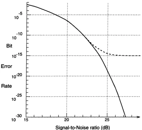
By symmetry, the same analysis applies when pt = L. Figure 4-2 shows a plot of BER values given by Equation 4.1.

Note, however, that this idealized analysis will eventually break down at some point. When the power level is sufficiently high, the model developed above breaks down and other error sources become apparent, causing an 'error floor' in the BER vs. signal-to-noise ratio curve. The dashed line in Figure 4-2 is an illustration of such a floor.

In an optical link (especially with a power-inefficient transmission medium), the tradeoff between optical power and BER (lower power - higher BER) can be quite important. The optical sources require extremely fast electrical drivers, and the higher

(37)

-5 10 -10 10 Bit 10-15 Error 10-20 Rate -25 10 -30 10 15 20 25 Signal-to-Noise ratio (dB)

Figure 4-2: Error rate vs. Signal-to-noise ratio

the power required of the drivers, the more difficult their design becomes. Also, there is a power vs. reliability tradeoff in semiconductor lasers (lower power - higher reliability).

[The power-.BER tradeoff will also become important in Section 7, when I discuss intelligent control of laser drive power. In that case, I rely on the monotonic nature of this tradeoff to implement a power-control feedback loop with data link BER as the feedback variable.]

Generally, one needs extremely low error rates in a multiprocessor network, since an undetected error can be catastrophic. In Section 8.1, we derive a maximum tolerable BER of 10-23 for a prototype network. The best achievable BER values now are around 10- 15 _{[3], and even these levels are only possible with painstaking care in designing}

every part of the optical channel.

How then can one tolerate an optical network in a multiprocessor? As we shall see in Section 6, a simple error-control coding scheme can solve this dilemma quite neatly, provided that a usable (<10- 7, for example) bit-error-rate can be maintained.

(Chapter 6 gives a strategies for maintaining such error rates as the system ages.) In

... ... ...

... ... ... ...

.-

.

(38)

addition to making optical links usable in multiprocessors, error-control coding can also make their design and implementation much simpler and more cost-effective, by relaxing the otherwise stringent error-rate requirements.

4.1.1 Assumptions of the Analysis

The most fundamental assumption I shall make in my analysis of reliability solutions is that errors in different bit positions are independent. Since I am suggesting a system with wide optical channels, having separate optical channels for each bit, the assumption is quite plausible to a first order approximation.

However, I will be pushing this independence assumption very hard in my error-control analysis. Any significant error correlation between channels (for example, electromagnetic interference between channels at the receiver module) might compro-mise my error-control results. (On the other hand, such correlation might simplify the drive-control tasks addressed in Chapter 6, since one might only have to control the drive level on a per-module basis, instead of a per-laser basis).

Since such error problems are likely to be implementation-specific, I shall merely note the possibility of such problems, and conduct my subsequent analyses under the independent-error assumption.

4.2 Hard Failure

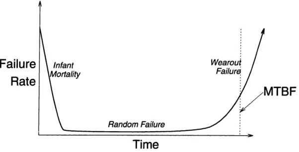
All electronic components degrade with age. Figure 4-3 shows the typical relationship (called the 'bathtub curve') between age and failure rate for any electronic component. Note that the entire curve is customarily characterized by one number: 'MTBF', an ambiguous acronym which can mean either mean or median time between failures. In this thesis, I shall generally consider MTBF to refer to the median time, and I will make it clear when the other sense is meant and the distinction is important. (In this case, MTTF, mean/median time to fail, is more appropriate, but we will use the more common term.)

Initially, there is a high failure rate due to flawed components ('infant mortality'). There follows a long period of few, randomly-distributed failures ('random failure'). Finally there is an increasing rate again ('wearout failure'), as the component aging

(39)

Failure

Rate

MTBF

Time

Figure 4-3: Component failure rate vs. time processes begin to take their toll.

Infant mortality can be controlled by proper screening and burn-in procedures [32] before the system begins operation. Random and wearout failures, however, must be handled in the field, either by fault-tolerant redundancy schemes, or by repair.

Unfortunately, semiconductor lasers tend to degrade faster than most other compo-nents in an optical communication network, so their failures will tend to dominate the failure characteristics of the system. I will therefore examine the nature of semicon-ductor laser failure, considering wearout failures in this section, and random failures in Section 4.2.2.

4.2.1 Gradual wearout

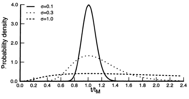
There are numerous aging processes which lead to wearout failure in semiconductor lasers [4], but they can collectively be modeled by a log-normal lifetime distribution, where log(lifetime) is a Gaussian random variable. If we let te denote the wearout lifetime of an individual laser, then the probability distribution of te will be given by

1

-In2(t/tM)

pt(t) = 7 e 2a2 (4.2)

where tM is the median lifetime, and a is the standard deviation. Figure 4-4 shows the shape of the log-normal distribution, for various values of a.

(40)

4.0 "F 3.0 C 2.0 2 .0 C_ 0. nn a=0.1 a=0.3 0.0 0.2 0.4 0.6 0.8 1.0 1.2 1.4 1.6 1.8 2.0 2.2 2.4 t/tM

Figure 4-4: Log-normal probability distributions

acronyms such as MTBF can be misleading. We can see that for larger values of a, the distribution is skewed toward larger values of te, and the mean lifetime will be considerably larger than the median. For example, with a = 0.4, the mean lifetime is 144% of the median.]

An important aspect of Figure 4-4 is that all of the curves are skewed away from time t = 0. This is why, for multiple lasers, the simplistic relation in Equation 1.1 does not apply. What relation does apply to wearout failures in multiple lasers? We shall answer this in Chapter 8, when we consider system-level solutions to the failure problem.

Laser wearout vs. time

Taken as a whole, the lifetimes of lasers in a system are random, and follow the probability density given in Equation 4.2. Taken individually, each laser has its own deterministic wearout lifetime. When this time comes, how does the wearout manifest itself?

Wearout failures are not instantaneous; they occur quite gradually. As a laser wears out, its light output gradually decreases for the same drive current. (Or,

(41)

Laser Output

Aging Time

Figure 4-5: Laser wearout vs. time

versely, the drive current required to maintain the same light output slowly increases). Laser MTBF figures are obtained by setting an arbitrary wearout criterion, such as a 50% output power decrease or a 100% drive current increase, and declaring a laser 'failed' when this criterion is reached. However, the gradual degradation continues considerably beyond this point, until finally the laser stops lasing. Figure 4-5 illus-trates this concept in the case of constant laser drive current.

The light output of a semiconductor laser is a linear function of the drive current

(ID) in excess of the threshold current (Ith) for that laser, that is

Laser light output cX ID - Ith (4.3)

The wearout processes generally manifest themselves as a gradual increase in threshold current. Using Ith(t) to denote threshold current as a function of time, we can model this gradual increase as

Ith(t) - Ith(O)

Ith(O)

where n is a constant characteristic of the particular laser type used (n ? 0.5 [33]). Letting a denote the drive current increase used for calculating the laser lifetime

te (for example, a 50% increase means a = 0.5), and letting Io denote the initial drive current used, we have

Control and reliability of optical networks in multiprocessors