HAL Id: hal-01330414
https://hal.inria.fr/hal-01330414
Submitted on 10 Jun 2016
HAL is a multi-disciplinary open access
archive for the deposit and dissemination of
sci-entific research documents, whether they are
pub-lished or not. The documents may come from
teaching and research institutions in France or
abroad, or from public or private research centers.
L’archive ouverte pluridisciplinaire HAL, est
destinée au dépôt et à la diffusion de documents
scientifiques de niveau recherche, publiés ou non,
émanant des établissements d’enseignement et de
recherche français ou étrangers, des laboratoires
publics ou privés.
Axioms for Information Leakage
Mário S. Alvim, Konstantinos Chatzikokolakis, Annabelle Mciver, Carroll
Morgan, Catuscia Palamidessi, Geoffrey Smith
To cite this version:
Mário S. Alvim, Konstantinos Chatzikokolakis, Annabelle Mciver, Carroll Morgan, Catuscia
Palamidessi, et al.. Axioms for Information Leakage. 29th Computer Security Foundations
Sym-posium (CSF 2016), IEEE, Jun 2016, Lisbon, Portugal. pp.16. �hal-01330414�
Axioms for Information Leakage
M´ario S. Alvim
∗Konstantinos Chatzikokolakis
†Annabelle McIver
‡Carroll Morgan
§Catuscia Palamidessi
†Geoffrey Smith
¶∗ Computer Science Department
Universidade Federal de Minas Gerais
† CNRS, Inria, and
´
Ecole Polytechnique
‡Department of Computing
Macquarie University
§ School of Computer Science & Engineering
University of New South Wales, and Data61
¶School of Computing & Information Sciences
Florida International University
Abstract—Quantitative information flow aims to assess and control the leakage of sensitive information by computer systems. A key insight in this area is that no single leakage measure is appropriate in all operational scenarios; as a result, many leakage measures have been proposed, with many different properties. To clarify this complex situation, this paper studies information leakage axiomatically, showing important dependencies among different axioms. It also establishes a completeness result about the𝑔-leakage family, showing that any leakage measure satisfying certain intuitively-reasonable properties can be expressed as a 𝑔-leakage.
Index Terms—information flow, 𝑔-vulnerability, information theory, confidentiality.
I. INTRODUCTION
The theory of quantitative information flow has seen rapid development over the past decade, motivated by the need for rigorous techniques to assess and control the leakage of sensitive information by computer systems. The starting point of this theory is the modeling of a secret as something whose value is known to the adversary only as a prior probability
distribution 𝜋. This immediately suggests that the “amount”
of secrecy might be quantified based on 𝜋, where intuitively a uniform 𝜋 would mean “more” secrecy and a biased 𝜋 would mean “less” secrecy. But how, precisely, should the quantification be done?
Early work in this area (e.g., [1]) adopted classic information-theoretic measures like Shannon-entropy [2] and
guessing-entropy [3]. But these can be quite misleading in a
security context, because they can be arbitrarily high even if
𝜋 assigns a large probability to one of the secret’s possible
values, giving the adversary a large chance of guessing that secret correctly in just one try. This led to the introduction of Bayes vulnerability [4], which is simply the maximum probability that𝜋 assigns to any of the possible values of the secret. Bayes vulnerability indeed measures a basic security threat, but it implicitly assumes an operational scenario where the adversary must guess the secret exactly, in one try. There are of course many other possible scenarios, including those where the adversary benefits by guessing a part or a property of the secret or by guessing the secret within three tries, or where the adversary is penalized for making an incorrect guess. This led to the introduction of 𝑔-vulnerability [5], which uses gain functions𝑔 to model the operational scenario,
enabling specific𝑔-vulnerabilities to be tailored to each of the above scenarios, and many others as well.1
This situation may however strike us as a bit of a zoo. We have a multitude of exotic vulnerability measures, but perhaps no clear sense of what a vulnerability measure ought to be. Are all the𝑔-vulnerabilities “reasonable”? Are there “reasonable” vulnerability measures that we are missing?
The situation becomes more complex when we turn our at-tention to systems. We model systems as information-theoretic
channels, and the crucial insight, reviewed in Section II-B
below, is that each possible output of a channel allows the adversary to update the prior distribution 𝜋 to a posterior
distribution, where the posterior distribution itself has a
prob-ability that depends on the probprob-ability of the output. Hence a channel is a mapping from prior distributions to distributions
on posterior distributions, called hyper-distributions [6].
In assessing posterior vulnerabilities, by which we mean the vulnerability after the adversary sees the channel output, we have a number of choices. It is natural to consider the vulnerability of each of the posterior distributions, and take the
average, weighted by the probabilities of the posterior
distribu-tions. Or (if we are pessimistic) we might take the maximum. Next we can define the leakage caused by the channel by comparing the posterior vulnerability and prior vulnerability, either multiplicatively or additively. These choices, together with the multitude of vulnerability measures, lead us to many different leakage measures, with many different properties. Is there a systematic way to understand them? Can we bring order to the zoo?
Such questions motivate the axiomatic study that we un-dertake in this paper. We consider a set of axioms that characterize intuitively-reasonable properties that vulnerability measures might satisfy, separately considering axioms for prior vulnerability (Section IV) and axioms for posterior vulner-ability and for the relationship between prior and posterior vulnerability (Section V). Addressing this relationship is an important novelty of our axiomatization, as compared with
1Note that entropies measure secrecy from the point of view of the user (i.e., more entropy means more secrecy), while vulnerabilities measure secrecy from the point of view of the adversary (i.e., more vulnerability means less secrecy). The two perspectives are complementary, but to avoid confusion this paper focuses almost always on the vulnerability perspective.
previous axiomatizations of entropy (such as [2], [7], [8]), which considered only prior entropy, or the axiomatization of
utility by Kifer and Lin [9], which considers posterior utility
without investigating its relation to prior utility. As a result, our axiomatization is able to consider properties of leakage, usually defined in terms of comparison between the posterior and prior vulnerabilities.2
The main contributions of this paper are of two kinds. One kind involves showing interesting dependencies among the var-ious axioms. For instance, under axiom averaging for posterior vulnerability, we prove in Section V that three other axioms are equivalent: convexity, monotonicity (i.e., non-negativity of leakage), and the data-processing inequality. Convexity is the property that prior vulnerability is a convex function from distributions to reals; what is striking here is that it a property that might not be intuitively considered “fundamental”, yet our equivalence (assuming averaging) shows that it is. We also show an equivalence under the alternative axiom maximum for posterior vulnerability, which then involves quasi-convexity.
A second kind of contribution justifies the significance of 𝑔-vulnerability. Focusing on the axioms of convexity and
continuity for prior vulnerability, we consider the class of all
functions from distributions to reals that satisfy them, proving in Section IV that this class exactly coincides with the class of 𝑔-vulnerabilities. This soundness and completeness result shows that if we accept averaging, continuity, and convexity (or monotonicity or the data-processing inequality) then prior vulnerabilities are exactly 𝑔-vulnerabilities.
The rest of the paper is structured as follows: Section II reviews the basic concepts of quantitative information flow, Section III sets up the framework of our axiomatization, and Sections IV and V discuss axioms for prior and posterior vulnerabilites, respectively. Section VI provides some discus-sion, Section VII gives an abstract categorical perspective, Section VIII discusses related work, and Section IX concludes.
II. PRELIMINARIES
We now review some basic notions from quantitative infor-mation flow. A secret is something whose value is known to the adversary only as a prior probability distribution 𝜋: there are various ways for measuring what we will call its
vulnera-bility. A channel models systems with observable behavior that
changes the adversary’s probabilistic knowledge, making the secret more vulnerable and hence causing information leakage.
A. Secrets and vulnerability
The starting point of computer security is information that we wish to keep secret, such as a user’s password, social security number or current location. An adversary typically does not know the value of the secret, but still possesses some
2We should however clarify that we do not view axiomatics as a matter of identifying “self-evident” truths. A variety of axioms may appear intuitively reasonable, so while it is sensible to consider intuitive justifications for them, such justifications should not be considered absolute. Rather we see the value of axiomatics as consisting more in understanding the logical dependencies among different properties, so that we might (for instance) identify a minimal set of axioms that is sufficient to imply all the properties that we care about.
probabilistic information about it, captured by a probability
distribution called the prior. We denote by 𝒳 the finite set of possible secret values and by 𝔻𝒳 the set of probability distributions over 𝒳 . A prior 𝜋∈𝔻𝒳 could either reflect a probabilistic procedure for choosing the secret—e.g., the prob-ability of choosing a certain password—, or it could capture any knowledge the adversary possesses on the population the user comes from—e.g., a young person is likely to be located at a popular bar on Saturday night.
The prior𝜋 plays a central role at measuring how vulnerable a secret is. For instance, choosing short passwords is not vulnerable because of their length (prefixing passwords with a thousand zeroes does not necessarily render them more secure), but because each password has a high probability of being chosen. To obtain a concrete vulnerability measure one needs to consider an operational scenario describing the adversary’s capabilities and goals; vulnerability then measures the adversary’s expected success in this scenario.
Bayes-vulnerability [4] considers an adversary trying to
guess the secret in one try and measures the threat as the probability of the guess being correct. Knowing a prior𝜋, a
rational adversary will guess a secret to which it assigns the highest probability: hence Bayes-vulnerability is given by
𝑉𝑏(𝜋) = max𝑥∈𝒳 𝜋𝑥 ,
where we write 𝜋𝑥 for the probability 𝜋 assigns to 𝑥. Note that Bayes-vulnerability is called simply “vulnerability” in [4], and is the basic notion behind min-entropy, defined as
𝐻∞(𝜋) = − lg 𝑉𝑏(𝜋). It is also the converse of the adversary’s
probability of error, also called Bayes-risk in the area of hypothesis testing [10].
Guessing-entropy [3] considers an adversary trying to guess
the secret in an unlimited number of tries, and measures the adversary’s uncertainty as the number of guesses needed on average. The best strategy is to try secrets in non-increasing order of probability: if𝑥𝑖is an indexing of𝒳 in such an order, then guessing-entropy is given by
𝐺(𝜋) = ∑𝑖𝑖 𝜋𝑥𝑖 .
Shannon-entropy [2] considers an adversary who tries to
infer the secret using Boolean questions (i.e., of the form “does
𝑥 belong to a certain subset 𝒳′ of 𝒳 ?”) and measures the
adversary’s uncertainty as the number of questions needed on average. It can be shown that the best strategy is at each step to split the secret space in sets of equal probability (as far as possible). Under this strategy, a secret 𝑥 will be guessed in − lg 𝜋𝑥 steps, hence on average the number of questions needed is
𝐻(𝜋) = −∑𝑥∈𝒳 𝜋𝑥lg 𝜋𝑥 .
Note that Bayes-vulnerability measures the threat to the secret (the higher the better for the adversary). On the other hand, guessing- and Shannon-entropy measure the adversary’s
uncertainty about the secret (the lower the better for the
Although the operational scenarios described above capture realistic threats for the secret, one could envision a variety of alternative threats we might also be worried about. For instance, an adversary might be interested in guessing only
part of the secret, an approximate value of the secret, a property of the secret or guessing the secret in a fixed
number of tries. It is for this reason that the more general
𝑔-vulnerability framework [5] was proposed: it allows one to
adapt to many different adversarial models.
Its operational scenario is parametrized by a set 𝒲 of
guesses (possibly infinite) that the adversary can make about
the secret, and a gain function𝑔: 𝒲×𝒳 →ℝ. The gain 𝑔(𝑤, 𝑥) expresses the adversary’s benefit for having made the guess
𝑤 when the actual secret is 𝑥. The 𝑔-vulnerability function
measures the threat as the adversary’s expected gain for an optimal choice of guess 𝑤:
𝑉𝑔(𝜋) = sup
𝑤∈𝒲
∑
𝑥∈𝒳 𝜋𝑥𝑔(𝑤, 𝑥) . (1)
Regarding the set 𝒲 of allowable guesses, one might assume that this should just be𝒳 , the set of possible values of the secret. This is in fact too restrictive: the adversary’s goal might be to guess a piece of the secret, or a value close to the secret, or some property of the secret. As a consequence we allow an arbitrary set of guesses, possibly infinite, and make (almost) no restrictions on the values of𝑔. In particular, a negative value of 𝑔(𝑤, 𝑥) expresses situations when the adversary is penalized for making a particular guess under a particular secret; such values are essential for obtaining the results of Section IV-B. We do however impose one restriction on 𝑔, that for each prior 𝜋 there is at least one guess that gives non-negative gain. This essentially forces𝑉𝑔to be non-negative, although individual guesses (i.e particular 𝑤’s) can still give negative gain.
Note that, as its name suggests,𝑉𝑔 is a measure of vulner-ability, i.e., of the threat to the secret. An equally expressive alternative is to define an “uncertainty” measure similarly, but using a loss function𝑙 instead of a gain function and assuming that the adversary wants to minimize loss. The uncertainty measure, parametrized by 𝑙, can be then defined dually as
𝑈𝑙(𝜋) = inf𝑤∈𝒲∑𝑥∈𝒳 𝜋𝑥𝑙(𝑤, 𝑥), and is often called
Bayes-risk in the area of decision theory.
Due to the flexibility of gain functions,𝑔-vulnerability is a very expressive framework, one that can capture a great variety of operational scenarios. This raises the natural question of which other vulnerability measures are expressible in this framework. Bayes-vulnerability is a straightforward example, captured by guessing the exact secret, i.e., taking𝒲=𝒳 , and using the identity gain function defined as 𝑔𝑖𝑑(𝑤, 𝑥) = 1 iff
𝑤=𝑥 and 0 otherwise.
Guessing-entropy can be also captured in this framework [11], [12], this time using a loss function since it’s an un-certainty measure. The adversary in this case tries to guess a
permutation of𝒳 , i.e., the order in which secrets are chosen in
the operational scenario of guessing-entropy. We can naturally define the loss𝑙(𝑤, 𝑥) as the index of 𝑥 in 𝑤, i.e. the number
of guesses to find 𝑥, and using this loss function we get
𝑈𝑙(𝜋) = 𝐺(𝜋).
Similarly, in the case of Shannon-entropy, the adversary tries to guess a strategy for constructing his questions. Strategies can be described as probability distributions: at each step ques-tions split the search space into subsets of as even probability as possible. Hence, guesses are𝒲=𝔻𝒳 , and the loss can be defined as 𝑙(𝑤, 𝑥) = − lg 𝑤𝑥 (the number of steps needed to find𝑥 under the strategy 𝑤). Since the best strategy is to take
𝑤=𝜋 itself, it can be shown [11] that under this loss function 𝑈𝑙(𝜋) = 𝐻(𝜋).
In Section IV-B we show that 𝑔-vulnerability exactly co-incides with the generic class of continuous and convex vulnerability functions.
B. Channels, hypers and leakage
So far we have considered secrets for which a probabilistic prior is known, and have discussed different ways for measur-ing their vulnerability. We now turn our attention to systems, which are programs or protocols processing secret information and producing some observable behavior. Examples of such systems are password-checkers, implementations of cryptosys-tems, and anonymity protocols.
A system can be modeled as an (information theoretic)
channel, a triple(𝒳 , 𝒴, 𝐶), where 𝒳 , 𝒴 are finite sets of
(se-cret) input values and (observable) output values respectively and𝐶 is a ∣𝒳 ∣×∣𝒴∣ channel matrix in which each entry 𝐶𝑥,𝑦 corresponds to the probability of the channel producing output
𝑦 when the input is 𝑥. Hence each row of 𝐶 is a probability
distribution over 𝒴 (entries are non-negative and sum to 1). A channel is deterministic iff each row contains a single 1 identifying the only possible output for that input.
It is typically assumed that the adversary knows how the system works, i.e. knows the channel matrix𝐶. Knowing also the prior distribution 𝜋, the adversary can compute the joint distribution𝑝(𝑥, 𝑦)=𝜋𝑥𝐶𝑥,𝑦on𝒳 ×𝒴, producing joint random variables𝑋, 𝑌 with marginal probabilities 𝑝(𝑥) =∑𝑦𝑝(𝑥, 𝑦) and𝑝(𝑦) =∑𝑥𝑝(𝑥, 𝑦), and conditional probabilities 𝑝(𝑦∣𝑥) =
𝑝(𝑥,𝑦)/𝑝(𝑥) (if 𝑝(𝑥) is non-zero) and 𝑝(𝑥∣𝑦) = 𝑝(𝑥,𝑦)/𝑝(𝑦)
(if 𝑝(𝑦) is non-zero). Note that 𝑝𝑋𝑌 is the unique joint distribution that recovers 𝜋 and 𝐶, in that 𝑝(𝑥) = 𝜋𝑥 and
𝑝(𝑦 ∣ 𝑥) = 𝐶𝑥,𝑦 (if 𝑝(𝑥) is non-zero).3
For a given𝑦 (s.t. 𝑝(𝑦) is non-zero), the conditional proba-bilities𝑝(𝑥∣𝑦) for each 𝑥 ∈ 𝒳 form the posterior distribution
𝑝𝑋∣𝑦, which represents the posterior knowledge the adversary
has about input 𝑋 after observing output 𝑦.
Example 1. Given 𝒳 = {𝑥1, 𝑥2, 𝑥3}, 𝒴 = {𝑦1, 𝑦2, 𝑦3, 𝑦4},
and the channel matrix 𝐶 below, (the uniform) prior 𝜋 =
(1/3,1/3,1/3) combined with 𝐶 leads to joint matrix 𝐽:
𝐶 𝑦1 𝑦2 𝑦3 𝑦4 𝑥1 1 0 0 0 𝑥2 0 1/2 1/4 1/4 𝑥3 1/2 1/3 1/6 0 𝜋 −→ 𝐽 𝑦1 𝑦2 𝑦3 𝑦4 𝑥1 1/3 0 0 0 𝑥2 0 1/6 1/12 1/12 𝑥3 1/6 1/9 1/18 0
3When necessary to avoid ambiguity, we write distributions with subscripts, e.g.𝑝𝑋𝑌 or𝑝𝑌.
Summing columns of 𝐽 gives the marginal distributions 𝑝𝑌=(1/2,5/18,5/36,1/12), and normalizing gives the pos-terior distributions 𝑝𝑋∣𝑦1=(2/3, 0,1/3), 𝑝𝑋∣𝑦2=(0,3/5,2/5),
𝑝𝑋∣𝑦3=(0,3/5,2/5), and 𝑝𝑋∣𝑦4=(0, 1, 0).
The effect of a channel 𝐶 is to update the adversary’s knowledge from a prior 𝜋 to a collection of posteriors 𝑝𝑋∣𝑦, each occurring with probability 𝑝(𝑦). Hence, following [6], [13], we view a channel as producing a probability distribution over posteriors, called a hyper-distribution.4
A hyper (for short) on the input space 𝒳 is of type 𝔻2𝒳 , which stands for 𝔻(𝔻𝒳 ), a distribution on distributions on
𝒳 . The support of a hyper is the set of possible posteriors
that the action of channel 𝐶 on prior 𝜋 can produce: we call those posteriors inners. The probability assigned by the hyper to a particular inner is the marginal probability of the𝑦 that produced that inner. We call those probabilities the outer probabilities. We useΔ to denote a hyper, ⌈Δ⌉ for its support (the set of posteriors with non-zero probability),[𝜋] to denote the point-hyper assigning probability 1 to 𝜋, and [𝜋, 𝐶] to denote the hyper obtained by the action of 𝐶 on 𝜋. We say that[𝜋, 𝐶] is the result of pushing prior 𝜋 through channel 𝐶. In Example 1, the hyper [𝜋, 𝐶] assigns (outer) proba-bilities (1/2,15/36,1/12) to the (inner) posteriors (2/3, 0,1/3),
(0,3/5,2/5), and (0, 1, 0), respectively.5
Since the outcome of a channel is a hyper, it is natural to extend vulnerability measures from priors to hypers, obtain-ing a posterior vulnerability. For all measures described in Section II-A this has been done in a natural way by taking the vulnerability of each posterior and averaging them using the outer. Let Exp𝜋𝐹 :=∑𝑥𝜋𝑥𝐹 (𝑥) denote the expected
value of some random variable𝐹 : 𝒳 →𝑅 (where 𝑅 is usually
the reals ℝ but more generally can be a vector space) over a distribution 𝜋: 𝔻𝒳 . We can then define posterior
Bayes-vulnerability ˆ𝑉𝑏: 𝔻2𝒳 → ℝ+ as ˆ
𝑉𝑏Δ = ExpΔ𝑉𝑏 ,
and similarly for Shannon-entropy, guessing-entropy and 𝑔-vulnerability. For hypers [𝜋, 𝐶] produced by channels, from the above formula we can get an expression of each posterior vulnerability as a function of𝜋 and 𝐶, for instance,
ˆ
𝑉𝑏[𝜋, 𝐶] = ∑𝑦 max𝑥𝜋𝑥𝐶𝑥,𝑦 , and
ˆ
𝑉𝑔[𝜋, 𝐶] = ∑𝑦 sup𝑤∑𝑥𝜋𝑥𝐶𝑥,𝑦𝑔(𝑤, 𝑥) .
Note that, for point-hypers, we have by construction that ˆ
𝑉𝑏[𝜋] = 𝑉𝑏(𝜋), and similarly for the other measures.
Finally, the execution of a system is expected to disclose information about the secret to the adversary, and the
infor-mation leakage of a channel 𝐶 for a prior 𝜋 is defined by
comparing the vulnerability of the prior 𝜋—the adversary’s
4Mappings of priors to hypers are called abstract channels in [13]. 5There might be fewer posteriors in the support of hyper[𝜋, 𝐶] than there are columns in the joint distribution𝑝𝑋,𝑌 from which it is derived, because if several columns of𝑝𝑋,𝑌 normalize to the same posterior then the hyper will automatically coalesce them [13]. Columns𝑦2and𝑦3were coalesced in this case.
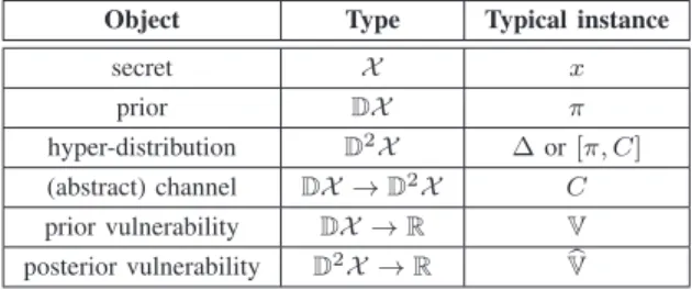
Object Type Typical instance
secret 𝒳 𝑥 prior 𝔻𝒳 𝜋 hyper-distribution 𝔻2𝒳 Δ or [𝜋, 𝐶] (abstract) channel 𝔻𝒳 → 𝔻2𝒳 𝐶 prior vulnerability 𝔻𝒳 → ℝ 𝕍 posterior vulnerability 𝔻2𝒳 → ℝ ˆ𝕍 TABLE I: Notation.
prior knowledge—and that of[𝜋, 𝐶]—the adversary’s posterior knowledge. The comparison is typically done either additively or multiplicatively, giving rise to two versions of leakage:
additive:ℒ+𝑏(𝜋, 𝐶) = ˆ𝑉𝑏[𝜋, 𝐶] − 𝑉𝑏(𝜋) , and (2) multiplicative:ℒ×𝑏 (𝜋, 𝐶) = lg (𝑉ˆ𝑏[𝜋,𝐶]/𝑉𝑏(𝜋)) . (3) Note thatℒ×𝑏(𝜋, 𝐶) is usually called min-entropy leakage [4]. Leakage can be similarly defined for all other measures.
III. AXIOMATIZATION
In Section II we discussed vulnerability measures obtained by quantifying the threat to the secret in a specific oper-ational scenario. Channels were then introduced, mapping prior distributions to hypers, and the vulnerability measures were naturally extended to posterior ones by averaging each posterior vulnerability over the hyper.
In this paper we take an alternative approach. Instead of constructing specific vulnerability measures, we consider generic vulnerability functions, that is, functions of type:
prior vulnerability: 𝕍 : 𝔻𝒳 → ℝ+, and posterior vulnerability: ˆ𝕍 : 𝔻2𝒳 → ℝ+.
We then introduce a variety of properties that “reasonable” vulnerabilities might be expected to have in terms of axioms, and study their consequences.
In Section IV we focus on the prior case and give axioms for prior vulnerabilities 𝕍 alone. We then show that taking convexity and continuity as our generic properties results in 𝑔-vulneraibility exactly. Then, in Section V, we turn our attention to axioms considering either both 𝕍 and ˆ𝕍, or posterior ˆ𝕍 alone. Moreover we study two ways of constructing ˆ𝕍 from 𝕍 and show that, in each case, several of the axioms become equivalent.
Note that the axioms purely affect the relationship between prior and posterior vulnerabilities, and are orthogonal to the way𝕍 and ˆ𝕍 are compared to measure leakage (e.g., multi-plicatively or additively). Moreover, although in this paper we consider axioms for vulnerability, dual axioms can be naturally stated for generic uncertainty measures.
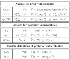
Table I summarizes the notation used through the paper, while Table II summarizes the axioms we consider.
IV. AXIOMATIZATION OF PRIOR VULNERABILITIES We now introduce axioms that deal solely with prior vul-nerabilities 𝕍.
Axioms for prior vulnerabilities
CNTY ∀𝜋: 𝕍 is a continuous function of 𝜋 CVX ∀∑𝑖𝑎𝑖𝜋𝑖: 𝕍(∑𝑖𝑎𝑖𝜋𝑖) ≤ ∑𝑖𝑎𝑖𝕍(𝜋𝑖) Q-CVX ∀∑𝑖𝑎𝑖𝜋𝑖: 𝕍(∑𝑖𝑎𝑖𝜋𝑖) ≤ max𝑖𝕍(𝜋𝑖)
Axioms for posterior vulnerabilities
NI ∀𝜋: 𝕍[𝜋] = 𝕍(𝜋)ˆ
DPI ∀𝜋, 𝐶, 𝑅: 𝕍[𝜋, 𝐶] ≥ ˆˆ 𝕍[𝜋, 𝐶𝑅] MONO ∀𝜋, 𝐶: 𝕍[𝜋, 𝐶] ≥ 𝕍(𝜋)ˆ
Possible definitions of posterior vulnerabilities
AVG ∀Δ: 𝕍Δ = Expˆ Δ𝕍
MAX ∀Δ: 𝕍Δ = maxˆ ⌈Δ⌉𝕍
TABLE II: Summary of axioms for pairs of prior/posterior vulnerabilities (𝕍, ˆ𝕍).
Continuity (CNTY). A vulnerability 𝕍 is a continuous
function of 𝜋 (w.r.t. the standard topology on 𝔻𝒳 ).
The CNTY axiom imposes that “small” changes on the prior 𝜋 should have a “small” effect on 𝕍. This formalizes the intuition that the adversary should not be infinitely risk-averse. For instance, the non-continuous function 𝕍(𝜋) = (1 if max𝑥𝜋𝑥≥ 𝜆 else 0) would correspond to an adversary
who requires the probability of guessing to be above a certain threshold in order to consider an attack effective. But this is an arguably unnatural behavior, the risk of changing the probability to 𝜆−𝜖, for an infinitesimal 𝜖, should not be arbitrarily large.
A convex combination of priors 𝜋1, . . . , 𝜋𝑛 is a sum ∑
𝑖𝑎𝑖𝜋𝑖 where 𝑎𝑖’s are non-negative reals adding up to 1.
Since 𝔻𝒳 is a convex set, a convex combination of priors is itself a prior.
Convexity (CVX). A vulnerability 𝕍 is a convex function
of 𝜋, that is for all convex combinations∑𝑖𝑎𝑖𝜋𝑖: 𝕍(∑𝑖𝑎𝑖𝜋𝑖) ≤ ∑𝑖𝑎𝑖𝕍(𝜋𝑖) .
This axiom can be interpreted as follows: imagine a “game” in which a secret (say a password) is drawn from two possible distributions 𝜋1 or 𝜋2. The choice of distributions is itself random: we first select 𝑖 ∈ {1, 2} at random, with 𝑖 = 1 having probability 𝑎1 and𝑖 = 2 probability 𝑎2= 1 − 𝑎1, and then use 𝜋𝑖 to draw the secret.
Now consider the following two scenarios for this game: in the first scenario, the value of 𝑖 is given to the adversary, so the actual prior the secret was drawn from is known. Using the information in 𝜋𝑖the adversary performs an attack, the expected success of which is measured by 𝕍(𝜋𝑖), so the expected measure of success overall will be∑𝑖𝑎𝑖𝕍(𝜋𝑖).
In the second scenario, 𝑖 is not disclosed to the adversary, who only knows that, on average, secrets are drawn from the prior ∑𝑖𝑎𝑖𝜋𝑖, hence the expected success of an attack will be measured by 𝕍(∑𝑖𝑎𝑖𝜋𝑖). CVX corresponds to the
intuition that, since in the first scenario the adversary has more information, the effectiveness of an attack can only be higher. Note that, in the definition of CVX, it is sufficient to use convex combinations of two priors, i.e., of the form 𝑎𝜋1+ (1 − 𝑎)𝜋2; we often use such combinations in proofs. Note
also that CVX actually implies continuity everywhere except on the boundary of the domain, i.e., on priors having an element with probability exactly0. CNTY explicitly requires continuity everywhere.
Since the vulnerabilities𝕍(𝜋𝑖) in the definition of CVX are weighted by the probabilities 𝑎𝑖, we could have cases when the expected vulnerability∑𝑖𝑎𝑖𝕍(𝜋𝑖) is small although some individual 𝕍(𝜋𝑖) is large. In such cases, one might argue that the bound imposed by CVX is too strict and could be loosened by requiring that 𝕍(∑𝑖𝑎𝑖𝜋𝑖) is only bounded by the maximum of the individual vulnerabilities. This weaker requirement is called quasiconvexity.
Quasiconvexity (Q-CVX). A vulnerability𝕍 is a
quasicon-vex function of𝜋, that is for all ∑𝑖𝑎𝑖𝜋𝑖: 𝕍(∑𝑖𝑎𝑖𝜋𝑖) ≤ max𝑖 𝕍(𝜋𝑖) .
In Section V we show that CVX and Q-CVX can be in fact obtained as consequences of fundamental axioms relating prior and posterior vulnerabilities, and specific choices for constructing ˆ𝕍.
In the remainder of this section we show that the vulner-ability functions satisfying CNTY and CVX are exactly those expressible as 𝑉𝑔 for some gain function 𝑔. We treat each direction separately; full proofs are given in Appendix A.
A. 𝑉𝑔 satisfies CNTYand CVX
We first show that any 𝑔-vulnerability satisfies CNTY and CVX. Let𝒲 be a possibly infinite set of guesses and 𝑔: 𝒲 ×
𝒳 → ℝ be a gain function. We start by expressing 𝑉𝑔 as the
supremum of a family of functions:
𝑉𝑔(𝜋) = sup
𝑤 𝑔𝑤(𝜋), where 𝑔𝑤(𝜋) =
∑
𝑥𝜋𝑥𝑔(𝑤, 𝑥) .
Intuitively, 𝑔𝑤 gives the expected gain for the specific guess
𝑤, as a function of 𝜋. Note that 𝑔𝑤 is linear on𝜋, hence both (trivially) convex and continuous.
The convexity of𝑉𝑔then follows from the fact that thesup of any family of convex functions is itself a convex function. On the other hand, showing continuity is more challenging, since the supremum of continuous functions is not necessarily continuous itself.
To show that𝑉𝑔 is continuous, we employ the concept of semi-continuity. Informally speaking, a function is upper (resp. lower) semi-continuous at 𝑥0 if, for values close to 𝑥0, the function is either close to 𝑓(𝑥0) or less than 𝑓(𝑥0) (resp. greater than 𝑓(𝑥0)).
Lower semi-continuity is obtained from the following proposition:
Proposition 2. If𝑓 is the supremum of a family of continuous
1
0 π1 π2
g(w,x2)
g(w,x1)
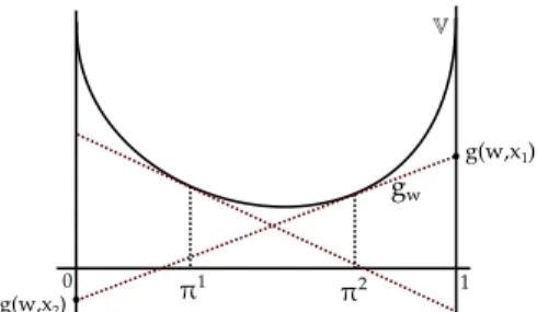
gw
Fig. 1: Supporting hyperplanes on different priors
On the other hand, upper semi-continuity follows from the structure of the probability simplex and the Gale-Klee-Rockafellar theorem:
Theorem 3 (Gale-Klee-Rockafellar, [14]). If𝑓 is convex and
its domain is a polyhedron then it is upper semi-continuous.
Hence,𝑉𝑔is both lower semi-continuous (as the supremum of continuous functions) and upper semi-continuous (it is convex and𝔻𝒳 is a polyhedron), and any function satisfying both semi-continuities is necessarily continuous.
Corollary 4. Any𝑔-vulnerability 𝑉𝑔 satisfies CNTY,CVX. B. CNTYand CVXexactly characterize𝑉𝑔
Gain functions and 𝑔-vulnerability were introduced in [5], [6] in order to capture a variety of operational scenarios. Besides naturally retrieving Bayes-vulnerability as a special case, the flexibility of 𝑔-vulnerability allows us to retrieve other well-known entropy measures, such as Shannon- and guessing-entropy, using properly constructed gain functions [11], [12]. This suggests the question of how expressive 𝑔-vulnerabilities are in general.
Remarkably, it turns out that𝑔-vulnerabilities are expressive enough to capture any vulnerability function 𝕍 satisfying CNTY and CVX, although in the general case a countably infinite set 𝒲 of guesses might be needed.
Theorem 5. Let 𝕍 : 𝔻𝒳 → ℝ+ be a vulnerability function satisfyingCNTYandCVX. Then there exists a gain function𝑔 with a countable number of guesses such that 𝕍 = 𝑉𝑔.
The full proof is given in Appendix A; in the remainder of this section we try to convey the main arguments. A geometric view of gain functions is very helpful. Recall that
𝑔𝑤(𝜋), expressing the expected gain of a fixed guess 𝑤, is a linear function of 𝜋. A crucial observation is that the graph of 𝑔𝑤, that is the set of vectors {(𝜋, 𝑔𝑤(𝜋)) ∣ 𝜋 ∈ 𝔻𝒳 }, forms a hyperplane. Moreover, it can be shown that any such hyperplane6 can be obtained as the graph of𝑔𝑤 by properly
choosing the gains 𝑔(𝑤, 𝑥).
The correspondence between𝑔𝑤 and hyperplanes allows us to employ the supporting hyperplane theorem, which states that for any point 𝑠 at the boundary of a convex set 𝑆, there is a hyperplane passing through 𝑠 and leaving the whole set
6To be precise, only the hyperplanes not orthogonal to that of probability distributions: see the full proof for details.
𝑆 on the same half space. Since 𝕍 is a convex function, its epigraphepi𝕍 = {(𝜋, 𝑦) ∣ 𝑦 ≥ 𝕍(𝜋)} is a convex set. Given
any prior 𝜋∗, the point (𝜋∗, 𝕍(𝜋∗)) lies on the boundary of epi𝕍 hence there is a hyperplane passing from this point such that 𝕍 lies above the hyperplane. Supporting hyperplanes on different priors are illustrated in Figure 1.
Since such a hyperplane can be constructed for each prior, we are going to use priors as guesses, making 𝒲 = 𝔻𝒳 . For a guess 𝑤 ∈ 𝔻𝒳 we choose the gains 𝑔(𝑤, 𝑥) such that the graph of𝑔𝑤 is exactly the supporting hyperplane passing through(𝑤, 𝕍(𝑤)). Since 𝕍 lies above the hyperplane, we get:
𝑔𝑤(𝜋) = 𝕍(𝜋) for 𝑤 = 𝜋 , and
𝑔𝑤(𝜋) ≤ 𝕍(𝜋) for all𝜋 ∈ 𝔻𝒳 .
Finally, from the definition of𝑉𝑔 we have that
𝑉𝑔(𝜋) = sup
𝑤∈𝔻𝒳𝑔𝑤(𝜋) = 𝕍(𝜋) .
The restriction to a countable set of guesses can be obtained by limiting𝑤 to priors with rational elements, and using the continuity of𝑉𝑔. The details can be found in Appendix A.
V. AXIOMATIZATION OF POSTERIOR VULNERABILITIES In this section we consider axioms for posterior vulnerabil-ities and axioms that relate posterior and prior vulnerabilvulnerabil-ities. We investigate how different definitions of posterior vulner-abilities shape the interrelation among these postulates. We consider the following three axioms.
Non-interference (NI). The vulnerability of a point-hyper
equals the vulnerability of the unique inner of this hyper:
∀𝜋: ˆ𝕍[𝜋] = 𝕍(𝜋) .
This axiom means that an adversary who has learned with certainty that the secret follows distribution 𝜋 has the same amount of information𝕍(𝜋) one would have had from 𝜋 itself. This postulate can also be interpreted in terms of non-interference. A channel 𝐶NI is non-interfering if the result of pushing any prior 𝜋 through 𝐶NI is the point-hyper [𝜋], meaning that the adversary’s state of knowledge is never changed by the observation of the output of the channel. It is well known that a channel𝐶𝑁𝐼 is non-interfering iff all its rows are the same (see, for instance, [15]), so the simplest non-interfering channel is the null-channel, denoted here by ¯0, with only one column (i.e., every secret yields the same output). It can be easily verified that every non-interfering channel𝐶NI is equivalent to ¯0, since [𝜋, 𝐶NI] = [𝜋, ¯0] = [𝜋].
The NI axiom, then, is equivalent to stating that an adversary observing the output of a non-interfering channel does not gain or lose any information about the secret:
∀𝜋: ˆ𝕍[𝜋, ¯0] = 𝕍(𝜋) .
Data-processing inequality (DPI). Post-processing does
not increase vulnerability:7
∀𝜋, 𝐶, 𝑅: ˆ𝕍[𝜋, 𝐶] ≥ ˆ𝕍[𝜋, 𝐶𝑅] ,
7The data-processing inequality is a well well-known property of Shan-non mutual information [16]: if 𝑋→𝑌 →𝑍 forms a Markov chain, then
where the number of columns in matrix𝐶 is the same as the number of rows in matrix 𝑅.
This axiom can be interpreted as follows. Consider that a secret is fed into a channel𝐶, and the produced output is, then, post-processed by being fed into another channel𝑅 (naturally the input domain of𝑅 must be the same as the output domain of 𝐶). Now consider two adversaries 𝐴 and 𝐴′ such that 𝐴 can only observe the output of channel 𝐶, and 𝐴′ can only observe the output of the cascade 𝐶′ = 𝐶𝑅. For any given prior 𝜋 on secret values, 𝐴’s posterior knowledge about the secret is given by the hyper [𝜋, 𝐶], whereas that of 𝐴′’s is given by [𝜋, 𝐶′]. Note, however, that from 𝐴’s knowledge it is always possible to reconstruct𝐴′’s, but the converse is not necessarily true.8 Given this asymmetry, DPI formalizes that
a vulnerability ˆ𝕍 should not evaluate 𝐴’s information as any less than 𝐴′’s.
Monotonicity (MONO). Pushing a prior through a channel
does not decrease vulnerability:
∀𝜋, 𝐶: ˆ𝕍[𝜋, 𝐶] ≥ 𝕍(𝜋) .
One interpretation for this axiom is that by observing the output of a channel an adversary cannot lose information about the secret; in the worst case, the output can be ignored if it is not useful.9 A direct consequence of this axiom is
that, since posterior vulnerabilities are always greater than the corresponding prior vulnerabilities, additive and multiplicative versions of leakage as defined in Equations (2) and (3) are always non-negative.
Having presented the three axioms of NI, DPI and MONO, we discuss next how posterior vulnerabilities can be defined so to respect them. Differently from the case of prior vulner-abilities, in which the axioms considered (CVX and CNTY) were sufficient to determine 𝑔-vulnerabilities as the unique family of prior-measures that satisfy them, our axioms for posterior vulnerabilities do not determine explicitly a unique family of posterior vulnerabilities ˆ𝕍. In the following sections we consider alternative definitions of posterior vulnerabilities and discuss the interrelation of the axioms they induce.
A. Posterior vulnerability as expectation
As seen in Section II, the posterior versions of Shannon-, guessing-, and min-entropy, as well as of 𝑔-vulnerability, are all defined as the expectation of the corresponding prior measures applied to each posterior distribution, weighted by the probability of each posterior’s being realized. We will now consider the consequences of taking as an axiom the definition of posterior vulnerability as expectation.
8𝐴 can use 𝜋 and 𝐶 to compute [𝜋, 𝐶𝑅′] for any 𝑅′, including the
particular𝑅 used by 𝐴′. On the other hand,𝐴′only knows𝜋 and 𝐶′, and in general the decomposition of𝐶′into a cascade of two channels is not unique (i.e., there may be several pairs𝐶𝑖,𝑅𝑖of matrices satisfying𝐶′= 𝐶𝑖𝑅𝑖), so it is not always possible for𝐴′to uniquely recover𝐶 from 𝐶′and compute [𝜋, 𝐶].
9This axiom is a generalization of Shannon-entropy’s “information can’t
hurt” property [16]:𝐻(𝑋 ∣ 𝑌 ) ≤ 𝐻(𝑋), for all random variables 𝑋, 𝑌 .
(a) Defining ˆ𝕍 as AVG (b) Defining ˆ𝕍 as MAX
Fig. 2: Equivalence of axioms. The merging arrows indicate joint implication: for example, on the left-hand side we have that MONO+ AVG imply CVX.
Averaging (AVG). The vulnerability of a hyper is the
expected value, with respect to the outer distribution, of the vulnerabilities of its inners:
∀Δ: ˆ𝕍Δ = ExpΔ𝕍 ,
where the hyperΔ: 𝔻2𝒳 might result from Δ=[𝜋, 𝐶] for some
𝜋, 𝐶.
The main results of this section consist in demonstrating that by imposing AVG on a prior/posterior pair (𝕍, ˆ𝕍) of vulnerabilities, NI too is necessarily satisfied for this pair, and, furthermore, the axioms of CVX, DPI and MONO become equivalent to each other. Figure 2a illustrates these results.
Proposition 6 (AVG ⇒ NI). If a pair of prior/posterior
vulnerabilities(𝕍, ˆ𝕍) satisfies AVG, then it also satisfiesNI.
Proof: If AVG is assumed, for any prior𝜋 it is the case that ˆ𝕍[𝜋] = Exp[𝜋]𝕍 = 𝕍(𝜋), since [𝜋] is a point-hyper.
Proposition 7 (NI + DPI ⇒ MONO). If a pair of
prior/posterior vulnerabilities (𝕍, ˆ𝕍) satisfies NI and DPI, then it also satisfiesMONO.
Proof: For any𝜋, 𝐶, let ¯0 denote the non-interfering channel with only one column and as many rows as the columns of
𝐶. Then
ˆ𝕍[𝜋, 𝐶]
≥ ˆ𝕍[𝜋, 𝐶¯0] (by DPI)
= ˆ𝕍[𝜋, ¯0] (𝐶¯0 = ¯0)
= ˆ𝕍[𝜋] (since ¯0 has only one column)
= 𝕍(𝜋) (by NI)
Proposition 8 (AVG + MONO ⇒ CVX). If a pair of
prior/posterior vulnerabilities(𝕍, ˆ𝕍) satisfiesAVGandMONO, then it also satisfiesCVX.
Proof: Let𝒳 = {𝑥1, . . . , 𝑥𝑛} be a finite set, and let 𝜋1 and
𝜋2 be distributions over 𝒳 . Let 0≤𝑎≤1, so that also 𝜋3 =
channel matrix 𝐶∗ = ⎡ ⎢ ⎢ ⎢ ⎢ ⎢ ⎢ ⎣ 𝑎𝜋1 1/𝜋13 (1−𝑎)𝜋21/𝜋31 .. . ... 𝑎𝜋1 𝑖/𝜋𝑖3 (1−𝑎)𝜋2𝑖/𝜋3𝑖 .. . ... 𝑎𝜋1 𝑛/𝜋𝑛3 (1−𝑎)𝜋2𝑛/𝜋3𝑛 ⎤ ⎥ ⎥ ⎥ ⎥ ⎥ ⎥ ⎦ . (4)
By pushing 𝜋3 through 𝐶∗ we obtain the hyper [𝜋3, 𝐶∗] with outer distribution(𝑎, 1−𝑎), and associated inners 𝜋1and
𝜋2. Since AVG is assumed, we have
ˆ𝕍[𝜋3, 𝐶∗] = 𝑎𝕍(𝜋1) + (1−𝑎)𝕍(𝜋2) . (5)
But note that by MONO, we also have
ˆ𝕍[𝜋3, 𝐶∗] ≥ 𝕍(𝜋3) = 𝕍(𝑎𝜋1+ (1−𝑎)𝜋2) . (6)
Taking (5) and (6) together, we obtain CVX.
For our next result, we will need the following lemma.
Lemma 9. Let 𝑋→𝑌 →𝑍 form a Markov chain with triply
joint distribution 𝑝(𝑥, 𝑦, 𝑧) = 𝑝(𝑥)𝑝(𝑦∣𝑥)𝑝(𝑧∣𝑦) for all
(𝑥, 𝑦, 𝑧) ∈ 𝒳 ×𝒴×𝒵. Then ∑𝑦𝑝(𝑦∣𝑧)𝑝(𝑥∣𝑦) = 𝑝(𝑥∣𝑧) for all𝑥, 𝑦, 𝑧.
Proof: First we note that the probability of 𝑧 depends only on the probability of 𝑦, and not 𝑥, so 𝑝(𝑧∣𝑥, 𝑦) = 𝑝(𝑧∣𝑦) for all 𝑥, 𝑦, 𝑧. Then we can use the fact that
𝑝(𝑦, 𝑧)𝑝(𝑥, 𝑦) = 𝑝(𝑥, 𝑦, 𝑧)𝑝(𝑦) (7) to derive: ∑ 𝑦𝑝(𝑦∣𝑧)𝑝(𝑥∣𝑦) = ∑𝑦 𝑝(𝑦,𝑧)𝑝(𝑥,𝑦)𝑝(𝑧)𝑝(𝑦) = ∑𝑦 𝑝(𝑥,𝑦,𝑧)𝑝(𝑦)𝑝(𝑧)𝑝(𝑦) (by Equation (7)) = ∑𝑦𝑝(𝑥, 𝑦∣𝑧) = 𝑝(𝑥∣𝑧)
Proposition 10 (AVG + CVX ⇒ DPI). If a pair of
prior/posterior vulnerabilities (𝕍, ˆ𝕍) satisfies AVGand CVX, then it also satisfies DPI.
Proof: Let𝒳 , 𝒴 and 𝒵 be sets of values. Let be 𝜋 be a prior on𝒳 , 𝐶 be a channel from 𝒳 to 𝒴, and 𝑅 be a channel from
𝒴 to 𝒵. Note that the cascading 𝐶𝑅 of channels 𝐶 and 𝑅 is
a channel from𝒳 to 𝒵.
Let 𝑝(𝑥, 𝑦, 𝑧) be the triply joint distribution defined as
𝑝(𝑥, 𝑦, 𝑧) = 𝜋𝑥𝐶𝑥,𝑦𝑅𝑦,𝑧 for all (𝑥, 𝑦, 𝑧) ∈ 𝒳 ×𝒴×𝒵. By construction, this distribution has the special Markov property that the probability of𝑧 depends only on the probability of 𝑦, and not 𝑥. Thus 𝑝(𝑧 ∣ 𝑥, 𝑦) = 𝑝(𝑧 ∣ 𝑦).
Note that, by pushing prior𝜋 through channel 𝐶, we obtain hyper[𝜋, 𝐶], in which the outer distribution on 𝑦 is 𝑝(𝑦), and the inners are 𝑝𝑋∣𝑦. Thus we can derive:
ˆ𝕍[𝜋, 𝐶] = ∑𝑦𝑝(𝑦)𝕍(𝑝𝑋∣𝑦) (by AVG) = ∑𝑦(∑𝑧𝑝(𝑧)𝑝(𝑦 ∣ 𝑧)) 𝕍(𝑝𝑋∣𝑦) = ∑𝑧𝑝(𝑧)∑𝑦𝑝(𝑦 ∣ 𝑧)𝕍(𝑝𝑋∣𝑦) ≥ ∑𝑧𝑝(𝑧)𝕍(∑𝑦𝑝(𝑦 ∣ 𝑧)𝑝𝑋∣𝑦 ) (by CVX) = ∑𝑧𝑝(𝑧)𝕍(𝑝𝑋∣𝑧) (by Lemma 9) = ˆ𝕍[𝜋, 𝐶𝑅] (by AVG)
Appendix B provides a concrete illustration of Proposition 10.
B. Posterior vulnerability as maximum
An important consequence of AVG is that an observable happening with very small probability will have a negligible effect on ˆ𝕍, even if it completely reveals the secret. If such a scenario is not acceptable, an alternative approach is to consider the maximum information that may be obtained from any single output of the channel—produced with non-zero probability—no matter how small this probability is. This conservative approach is employed, for instance, in the original definition of differential-privacy [17].
We shall now consider the consequences of taking the following definition of ˆ𝕍 as an axiom.
Maximum (MAX). The vulnerability of a hyper is the
maximum of the vulnerabilities of the inners in its support:
∀Δ: ˆ𝕍Δ = max
⌈Δ⌉ 𝕍 ,
where the hyperΔ: 𝔻2𝒳 might result from Δ=[𝜋, 𝐶] for some
𝜋, 𝐶.
The first result below shows that by imposing MAX on a prior/posterior pair(𝕍, ˆ𝕍) of vulnerabilities, NI is too satisfied for this pair.
Proposition 11. [MAX ⇒ NI] If a pair of prior/posterior vulnerabilities(𝕍, ˆ𝕍) satisfies MAX, then it also satisfiesNI.
Proof: If MAX is assumed, for any prior 𝜋 we will have ˆ𝕍[𝜋] = max⌈[𝜋]⌉𝕍 = 𝕍(𝜋), since [𝜋] is a point-hyper.
However, in contrast to the case of AVG, the symmetry among CVX, MONO and DPI is broken under MAX: although the axioms of MONO and DPI are still equivalent (shown later in this section, see Figure 2b), they are weaker than the axiom of CVX. This is demonstrated by the following example, show-ing a pair of prior/posterior vulnerabilities (𝕍, ˆ𝕍) satisfying MAX, MONO and DPI but not CVX.
Example 12 (MAX+MONO+DPI ∕⇒ CVX). Consider the pair
(𝕍1, ˆ𝕍1) such that for every prior 𝜋 and channel 𝐶:
𝕍1(𝜋) = 1 − ( min 𝑥 𝜋𝑥 )2 , and ˆ𝕍1[𝜋, 𝐶] = max ⌈[𝜋,𝐶]⌉𝕍1.
To see that𝕍1does not satisfyCVX, consider distributions 𝜋1= (0, 1) and 𝜋2(1/2,1/2), and its convex combination 𝜋3= 1/2𝜋1+1/2𝜋2= (1/4,3/4). We calculate 𝕍1(𝜋1) = 1−02= 1,
𝕍1(𝜋2) = 1 − (1/2)2 = 3/4, 𝕍1(𝜋3) = 1 − (1/4)2 = 15/16, and 1/2𝕍1(𝜋1) +1/2𝕍(𝜋2) =7/8 to conclude that𝕍1(𝜋3) >
The pair (𝕍1, ˆ𝕍1) satisfies MAX by construction. To show that it satisfies MONO and DPI, we first notice that 𝕍1 is quasiconvex. Using results from Figure 2b (proved later in this section), we conclude thatMONOand DPIare also satisfied.
The vulnerability function used in the counter-example above is quasiconvex. It turns out that this is not a coincidence: by replacing CVX with Q-CVX (a weaker property), the symmetry between the axioms can be restored. The remaining of this section establishes the equivalence of Q-CVX, MONO and DPI under MAX, as illustrated in Figure 2b.
Proposition 13. [MAX+ MONO ⇒ Q-CVX] If a pair of prior/posterior vulnerabilities(𝕍, ˆ𝕍) satisfiesMAXandMONO, then it also satisfies Q-CVX.
Proof: By contradiction, let us assume that (𝕍, ˆ𝕍) satisfy MAX and MONO, but does not satisfy Q-CVX.
Since Q-CVX is not satisfied, there must exist a value 0 ≤
𝑎 ≤ 1 and three distributions 𝜋1, 𝜋2, 𝜋3, such that 𝜋3 =
𝑎𝜋1+ (1 − 𝑎)𝜋2 and
𝕍(𝜋3) > max (𝕍(𝜋1), 𝕍(𝜋2)) . (8)
Consider the channel 𝐶∗ defined as in Equation (4). Then the hyper-distribution[𝜋3, 𝐶∗] has outer distribution (𝑎, 1−𝑎), and corresponding inner distributions 𝜋1 and 𝜋2. Since MAX is assumed, we have that
ˆ𝕍[𝜋3, 𝐶∗] = max (𝕍(𝜋1), 𝕍(𝜋2)) , (9)
and because we assumed MONO, we also have that
ˆ𝕍[𝜋3, 𝐶∗] ≥ 𝕍(𝜋3) . (10)
Equations (9) and (10) give 𝕍(𝜋3) ≤ max (𝕍(𝜋1), 𝕍(𝜋2)), which contradicts our assumption in Equation (8).
Proposition 14. [MAX + Q-CVX ⇒ DPI] If a pair
of prior/posterior vulnerabilities (𝕍, ˆ𝕍) satisfies MAX and
Q-CVX, then it also satisfiesDPI.
Proof: Let 𝜋 be a prior on 𝒳 , and 𝐶, 𝑅 be channels from 𝒳 to 𝒴 and from 𝒴 to 𝒵, respectively, with joint distribution𝑝(𝑥, 𝑦, 𝑧) defined in the same way as in the proof of Proposition 10.
Note that, by pushing prior 𝜋 through channel 𝐶𝑅, we obtain hyper [𝜋, 𝐶𝑅] in which the outer distribution on 𝑧 is
𝑝(𝑧), and the inner are 𝑝𝑋∣𝑧. Thus we can derive:
ˆ𝕍[𝜋, 𝐶𝑅]
= max𝑧𝕍(𝑝𝑋∣𝑧) (by MAX)
= max𝑧𝕍(∑𝑦𝑝(𝑦 ∣ 𝑧)𝑝𝑋∣𝑦 ) (by Lemma 9) ≤ max𝑧(max𝑦𝕍(𝑝𝑋∣𝑦) ) (by Q-CVX) = max𝑦𝕍(𝑝𝑋∣𝑦) = ˆ𝕍[𝜋, 𝐶] (by MAX)
Finally, note that, although Q-CVX is needed to recover the full equivalence of the axioms, CVX is strictly stronger than Q-CVX; hence, using a convex vulnerability measure (such as any 𝑉𝑔), MONO and DPI are still guaranteed under MAX.
Corollary 15. [MAX+CVX⇒MONO+DPI] If a pair(𝕍, ˆ𝕍) satisfies MAXandCVX, then it also satisfiesMONOand DPI.
Proof: Using the results of Figure 2b and the fact that CVX⇒ Q-CVX.
C. Other definitions of posterior vulnerabilities
In this section we explore the consequences of constraining posterior vulnerability more loosely than explicitly defining it as AVG or MAX. We require only that the posterior vulnerability cannot be greater than the vulnerability resulting from the most-informative channel output, nor less than the vulnera-bility resulting from the least-informative channel output.
Bounds (BNDS). The vulnerability of a hyper lies between
the minimum and the maximum of the vulnerabilities of the inners in its support:
∀Δ: min
⌈Δ⌉𝕍 ≤ ˆ𝕍Δ ≤ max⌈Δ⌉ 𝕍 ,
where the hyperΔ: 𝔻2𝒳 might result from Δ=[𝜋, 𝐶] for some
𝜋, 𝐶.
The next results show that, whereas BNDS is strong enough to ensure NI (Proposition 16), by replacing MAX with BNDS, the equivalence among Q-CVX, DPI and MONO no longer holds (Example 12).
Proposition 16 (BNDS ⇒ NI). If a pair of prior/posterior
vulnerabilities(𝕍, ˆ𝕍) satisfiesBNDS, then it also satisfiesNI.
Proof: If (𝕍, ˆ𝕍) satisfies BNDS, then min⌈Δ⌉𝕍 ≤ ˆ𝕍Δ ≤ max⌈Δ⌉𝕍 for every hyper Δ. Consider, then, the particular
case whenΔ = [𝜋]. Since [𝜋] is a point-hyper with inner 𝜋, we have that min⌈[𝜋]⌉𝕍 = max⌈[𝜋]⌉𝕍 = 𝕍(𝜋). This in turn implies that𝕍(𝜋) ≤ ˆ𝕍[𝜋] ≤ 𝕍(𝜋), which is NI.
The next example shows that under BNDS, not even CVX— which is stronger than Q-CVX—is sufficient to ensure MONO or DPI.
Example 17 (BNDS+ CVX ∕⇒ MONO or DPI). Consider the
pair(𝕍2, ˆ𝕍2) such that for every prior 𝜋 and hyper Δ:
𝕍2(𝜋) = max𝑥 𝜋𝑥, and
ˆ𝕍2Δ =(max⌈Δ⌉𝕍2+min⌈Δ⌉𝕍2)/2.
The pair (𝕍2, ˆ𝕍2) satisfies BNDS, since ˆ𝕍2 is the simple arithmetic average of maximum and minimum vulnerabilities of the inners. The pair (𝕍2, ˆ𝕍2) also satisfies CVX, since
𝕍2(𝜋) is just the Bayes vulnerability of 𝜋.
To see that the pair (𝕍2, ˆ𝕍2) does not satisfy MONO, consider prior 𝜋2= (9/10,1/10) and channel
𝐶2 = 8/09 1/1 .9
We can calculate that 𝕍2(𝜋2) = 9/10, and that [𝜋2, 𝐶2] has outer distribution(4/5,1/5), and inner distributions (1, 0) and
(1/2,1/2). Hence
ˆ𝕍2[𝜋2, 𝐶2] = (1+1/2)/2 = 3/4,
Now to see that the pair (𝕍2, ˆ𝕍2) does not satisfy DPI, consider the prior 𝜋3= (3/7,4/7) and the channels
𝐶3 =
1/3 2/3
1/4 3/4 and 𝑅3 =
1/4 3/4 3/4 1/4 .
We can calculate that[𝜋3, 𝐶3] has outer distribution (2/7,5/7),
and inners (1/2,1/2) and (2/5,3/5). Hence
ˆ𝕍2[𝜋3, 𝐶3] = (1/2+3/5)/2 = 11/20 = 0.55 .
On the other hand, the cascade 𝐶3𝑅3 yields the channel 𝐶3𝑅3 =
7/12 5/12 5/8 3/8 ,
and we can calculate [𝜋3, 𝐶3𝑅3] to have outer distribution
(17/28,11/28), and inners (7/17,10/17) and (5/11,6/11). Hence
ˆ𝕍[𝜋3, 𝐶
3𝑅3] = (10/17+6/11)/2 = 106/187 ≈ 0.567 ,
which makes ˆ𝕍[𝜋3, 𝐶3𝑅3] > ˆ𝕍[𝜋3, 𝐶3], violating DPI.
VI. DISCUSSION
In this section, we briefly discuss two applications of the results in Sections IV and V, showing how they can help to clarify the multitude of possible leakage measures.
One application concerns R´enyi entropy [8], a family of entropy measures defined by
𝐻𝛼(𝜋) = 1 − 𝛼1 lg(∑𝑥∈𝒳 𝜋𝛼 𝑥
)
for 0 ≤ 𝛼 ≤ ∞ (taking limits in the cases of 𝛼 = 1, which gives Shannon entropy, and𝛼 = ∞, which gives min-entropy). It would be natural to use R´enyi entropy to define a family of leakage measures by defining posterior R´enyi entropy ˆ𝐻𝛼 using AVG and defining R´enyi leakage by
ℒ𝛼(𝜋, 𝐶) = 𝐻𝛼(𝜋) − ˆ𝐻𝛼[𝜋, 𝐶] .
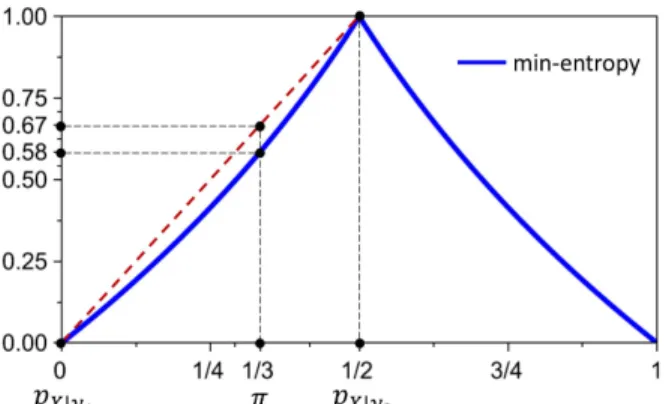
However, it turns out that 𝐻𝛼 is not concave for 𝛼 > 2. Therefore, by the dual version of Proposition 8, we find that R´enyi leakageℒ𝛼for𝛼 > 2 would sometimes be negative. As an illustration, Figure 3 shows how the nonconcavity of min-entropy𝐻∞can cause posterior min-entropy to be greater than prior min-entropy, giving negative min-entropy leakage.10
A second application concerns the robustness of the
compo-sition refinement relation ⊑∘ studied in [5], [6], [13]. Given channels 𝐶 and 𝐷, both taking input 𝑋, 𝐶 is composition refined by𝐷, written 𝐶 ⊑∘𝐷, if 𝐷 = 𝐶𝑅 for some “refining” channel 𝑅. As proved in [5], [13], composition refinement is
sound and complete for the strong 𝑔-leakage ordering: we
have𝐶 ⊑∘𝐷 iff the 𝑔-leakage of 𝐷 never exceeds that of 𝐶, regardless of the prior 𝜋 or gain function 𝑔. Still, we might worry that composition refinement implies a leakage ordering
only with respect to𝑔-leakage, leaving open the possibility that
the leakage ordering might conceivably fail for some yet-to-be defined leakage measure. But our Propositions 8 and 10 show
10Note that min-entropy leakage, as defined in [4], does not in fact define posterior min-entropy using AVG but instead by ˆ𝐻∞[𝜋, 𝐶] = − lg ˆ𝑉𝑏[𝜋, 𝐶].
Fig. 3: A picture showing how posterior min-entropy can be greater than prior min-entropy. Pushing prior 𝜋 = (1/3,2/3)
through channel𝐶 gives hyper [𝜋, 𝐶] with outer (1/3,2/3) and
inners 𝑝𝑋∣𝑦1 = (0, 1) and 𝑝𝑋∣𝑦2 = (1/2,1/2). So 𝐻∞(𝜋) = − lg2/3≈ 0.58 and ˆ𝐻∞[𝜋, 𝐶] =1/3⋅ 0 +2/3⋅ 1 ≈ 0.67.
that if the hypothetical new leakage measure is defined using AVG, and never gives negative leakage, then it also satisfies the data-processing inequality DPI. And hence composition refinement is also sound for the new leakage measure.
VII. ACATEGORICAL PERSPECTIVE
The axioms relating to Averaging are in fact instances of the monad laws proved by Giry for probabilistic computation [18], and in this section we give details. The benefit of this more general view is that it provides immediate access to well developed mathematical theories extending these results to infinite states and proper measures [19]. And this categorical perspective gives a direct connection to higher-order reasoning tools that dramatically simplify proofs, thereby leading directly to practical frameworks for calculating leakage [20].
The operator 𝔻 that takes a sample space 𝒳 to (discrete) distributions 𝔻𝒳 on that space is widely recognised as the “probability monad”, that is in effect a type constructor that obeys a small collection of laws shared by other, similar constructors like the powerset operatorℙ [18]. Each monad has two polymorphic functions𝜂, for “unit”, and 𝜇, for “multiply”, that interact with each other in elegant ways. For example in (the) ℙ (monad), unit has type 𝒳 →ℙ𝒳 and 𝜂𝑥 is {𝑥}, the singleton set containing just 𝑥; in 𝔻 we have type 𝒳 →𝔻𝒳 and𝜂𝑥 is [𝑥], the point-distribution on 𝑥. In ℙ, multiply 𝜇 is distributed union that takes a set of sets to the one set that is the union of them all, having thus the type ℙ2𝒳 →ℙ𝒳 ; and in 𝔻 we have (𝜇Δ)𝑥 = ∑𝛿: ⌈Δ⌉Δ𝛿𝛿𝑥, with 𝜇 thus of type𝔻2𝒳 →𝔻𝒳 and taking the outer-weighted average of all the inner distributions 𝛿 in the support of hyper Δ: it is the “weighted average” of the hyper. This means, for example, that𝜇[𝜋, 𝐶]=𝜋, i.e. that if you average the hyper produced by prior𝜋 and channel 𝐶 you get the prior back again.
Furthermore the monadic type-constructors are functors, meaning they can be applied to functions as well as to objects: thus for𝑓 in 𝒳 →𝒴 the function ℙ𝑓 of type ℙ𝒳 →ℙ𝒴 is such that for𝑋 in ℙ𝒳 we have 𝑓(𝑋) = {𝑓(𝑥) ∣ 𝑥∈𝑋} in ℙ𝒴. In