HAL Id: hal-00540388
https://hal.archives-ouvertes.fr/hal-00540388
Submitted on 26 Nov 2010
HAL is a multi-disciplinary open access
archive for the deposit and dissemination of
sci-entific research documents, whether they are
pub-lished or not. The documents may come from
teaching and research institutions in France or
abroad, or from public or private research centers.
L’archive ouverte pluridisciplinaire HAL, est
destinée au dépôt et à la diffusion de documents
scientifiques de niveau recherche, publiés ou non,
émanant des établissements d’enseignement et de
recherche français ou étrangers, des laboratoires
publics ou privés.
Effective temperatures of a heated Brownian particle
Laurent Joly, Samy Merabia, Jean-Louis Barrat
To cite this version:
Laurent Joly, Samy Merabia, Jean-Louis Barrat. Effective temperatures of a heated Brownian particle.
EPL - Europhysics Letters, European Physical Society/EDP Sciences/Società Italiana di Fisica/IOP
Publishing, 2011, 94, pp.50007. �10.1209/0295-5075/94/50007�. �hal-00540388�
Laurent Joly,∗ Samy Merabia,† and Jean-Louis Barrat‡
2
LPMCN, Universit´e de Lyon; UMR 5586 Universit´e Lyon 1 et CNRS, F-69622 Villeurbanne, France 3
(Dated: November 26, 2010) 4
We investigate various possible definitions of an effective temperature for a particularly simple 5
nonequilibrium stationary system, namely a heated Brownian particle suspended in a fluid. The 6
effective temperature based on the fluctuation dissipation ratio depends on the time scale under 7
consideration, so that a simple Langevin description of the heated particle is impossible. The short 8
and long time limits of this effective temperature are shown to be consistent with the temperatures 9
estimated from the kinetic energy and Einstein relation, respectively. The fluctuation theorem 10
provides still another definition of the temperature, which is shown to coincide with the short time 11
value of the fluctuation dissipation ratio. 12
PACS numbers: 05.70.Ln, 05.40.-a, 82.70.Dd, 47.11.Mn
13
In the recent years, so called “active colloids”, i.e.
col-14
loidal particles that exchange with their surroundings in
15
a non Brownian manner, have attracted considerable
at-16
tention from the statistical physics community [1]. These
17
systems are of interest as possible models for simple
liv-18
ing organisms, and the description of the corresponding
19
nonequilibrium states using the tools of standard
statis-20
tical physics raises a number of fundamental questions
21
[2, 3]. The most widely studied active colloids are those
22
that exchange momentum with the supporting solvent in
23
a non stochastic way, resulting into self propulsion. A less
24
studied possibility is that the colloid acts as a local heat
25
source and is constantly surrounded by a temperature
26
gradient. Experimentally [4], such a situation is achieved
27
when colloids are selectively heated by an external source
28
of radiation which is not absorbed by the solvent. If the
29
heat is removed far away from the particle, or, more
prac-30
tically, if the particle concentration is small enough that
31
the suspending fluid can be considered as a thermostat,
32
a simple nonequilibrium steady state is achieved. Each
33
colloidal particle is surrounded by a spherically
symmet-34
ric halo of hot fluid, and diffuses in an a priori Brownian
35
manner. The diffusion constant of such heated Brownian
36
particles was experimentally shown to be increased
com-37
pared to the one observed at equilibrium [4], and a semi
38
quantitative analysis of this enhancement was presented
39
in reference [5], based on an analysis of the temperature
40
dependence of the viscosity.
41
In this report, we use simulation to investigate in
de-42
tail the statistical physics of the simple non equilibrium
43
steady state (NESS) formed by a heated particle
sus-44
pended in a fluid. The most natural way of describing
45
such a system, in which the particles diffuse isotropically
46
in the surrounding fluid, is to make use of a Langevin
47
type equation for the center of mass velocity U ,
involv-48
ing in general a memory kernel ζ(t) and a random force
49 R(t): 50 MdU dt = − Z t −∞ ζ(t − s)U (s) ds + Fext+ R(t). (1)
In a system at thermal equilibrium at temperature T , the
51
correlations in the random force and the friction kernel
52
are related by the standard fluctuation dissipation
the-53
orem, hRα(t)Rβ(t′)i = δαβζ(|t − t′|)kBT [6]. Obviously
54
such a description is not expected to hold for a heated
55
particle, as the system is now out of equilibrium. A
gen-56
eralization of Eq. 1, involving a corrected fluctuation
57
dissipation relation with an effective temperature Teff
re-58
placing the equilibrium one, would however appear as a
59
natural hypothesis. In fact, such an approach was shown
60
to hold for sheared systems kept at a constant
tempera-61
ture by a uniform thermostat [7], or in the frame of the
62
particle for a particle driven at constant average speed [8].
63
The interpretation of recent experiments [3] also makes
64
implicitly use of such a description in describing the
sedi-65
mentation equilibrium of active particles, or in analyzing
66
the diffusion constant for hot Brownian motion [5].
67
The use of a Langevin equation with an effective
tem-68
perature has several direct consequences. The kinetic
69
energy associated with the center of mass, h12M U2i, is
70
necessarily equal to the effective temperature 32kBTeff.
71
The diffusion coefficient D and the mobility under the
72
influence of an external force µ = Ux/Fx are related by
73
an Einstein relation, D/µ = kBTeff [9]. More generally,
74
this relation can be seen as the steady state version of
75
the proportionality between the time dependent response
76
function to an external force, χ(t) = δUx(t)/δFx, and
77
the velocity autocorrelation in the nonequilibrium steady
78 state: 79 χ(t) = 1 kBTeff hUx(0)Ux(t)i. (2)
This relation was explored numerically for self propelled
80
particles in reference [2], and shown to be consistent with
81
the observed Einstein like relation. Independently of the
82
use of a specific Langevin model, this relation defines
83
an effective temperature trough a so called “fluctuation
84
dissipation ratio”. The applicability of an effective
tem-85
perature description is determined by the dependence of
86
this fluctuation dissipation ratio on time. We show in
87
the following that the time scale at which the fluctuation
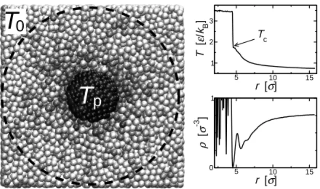
2 5 10 15 r [σ] 1 2 3 T [ ε /kB ] 5 10 15 r [σ] 0 1 ρ [ σ -3 ] Tc
T
p
T
0
FIG. 1. Left– Snapshot of the simulated system for Tp =
3.5ε/kB(T0= 0.75ε/kB); Gray levels indicate the kinetic
en-ergy of atoms. Right– Steady radial temperature and density profiles for this system.
dissipation ratio of a heated particle is determined indeed
89
matters, so that a single temperature description, even
90
in such a seemingly simple system, is problematic.
91
Finally, the use of a Langevin description with an
ef-92
fective temperature entails the validity of several
“fluc-93
tuation relations” [10], which have been the object of
94
numerous recent experimental and numerical tests, both
95
in equilibrium and nonequilibrium systems. The study of
96
the fluctuation relation for the heated particle constitutes
97
the last part of this report.
98
Our work is based on a direct molecular simulation
99
(MD) approach of a crystalline nanoparticle diffusing
100
in a liquid. The simulation were carried out using the
101
LAMMPS package [11]. Details of the model can be
102
found in previous works [12, 13], where we used this
103
system to investigate heat transfer from nanoparticles.
104
The particle was made of 555 atoms with a fcc
struc-105
ture, tied together using FENE bonds. The liquid was
106
made of ∼ 23000 atoms (Fig. 1). All liquid and solid
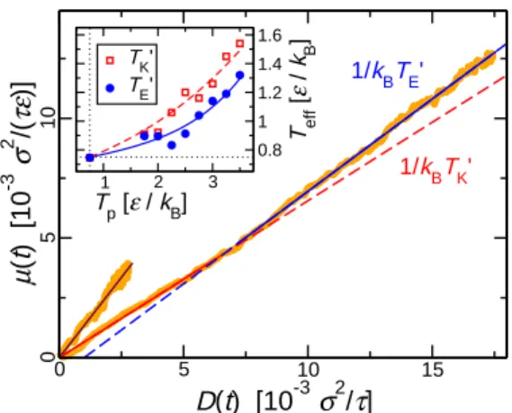
107 108
atoms interacted via the same Lennard-Jones (LJ)
po-109
tential v = 4ε[(σ/r)12− (σ/r)6], at the exclusion of solid
110
atoms directly bonded to each others. In the following,
111
all results will be given in LJ units, namely σ, ε/kB and
112
τ =pmσ2/ε for length, temperature and time,
respec-113
tively. The atoms in the solid particle were held at
con-114
stant temperature Tp using a Nos´e-Hoover thermostat,
115
after subtracting the velocity of the center of mass. In
116
order to mimic the bulk liquid – far from the particle
117
– acting as a thermal bath, a rescaling thermostat was
118
applied only to liquid atoms lying beyond 15σ from the
119
center of the particle (this condition being evaluated each
120
time the thermostat was applied), to keep them at
con-121
stant temperature T0 = 0.75ε/kB. This amounts to an
122
assumption that the temperature profile around the
par-123
ticle follows the latter instantaneously. This is a
reason-124
able assumption, as heat diffusion is much faster than
125
mass diffusion in our system: Dheat∼ 1σ2/τ [13], while
126
Dmass ∈ [0.002; 0.02]σ2/τ (Fig. 2). Finally the whole
127
system was kept at fixed pressure p = 0.0015ε/σ3
us-128
ing a Nos´e-Hoover barostat. Simulations were run over
129
typically 107 timesteps in order to accumulate enough
130
statistics.
131
In previous work, we have shown that nanoparticles
132
are able to sustain extremely high heat fluxes, via two
133
mechanisms: Firstly, interfacial thermal resistance at the
134
nanoscale generates significant temperature jumps at the
135
interface, i.e. the contact temperature Tcof the liquid at
136
the nanoparticle surface is much lower than the particle
137
temperature Tp(Fig. 1). Secondly, the large
curvature-138
induced Laplace pressure prevents the formation of a
va-139
por layer at the interface; At the highest temperatures,
140
only a stable depleted region is observed (Fig. 1).
141
Two approaches were used to measure the effective
142
temperature of the particle. We started by measuring
143
the kinetic temperature TK, related to the center of mass
144
velocity of the particle. Due to the finite ratio between
145
solid and liquid masses, care has to be taken to measure
146
the relative velocity between the solid nanoparticle and
147
the liquid Ui = Usi−Uli(i = x, y, z), with Usiand Ulithe
148
velocities of the solid and liquid centers of mass along the
149
i direction. TK was then given by 12kBTK = 12meffhUi2i,
150
where meff= msml/(ms+ ml) [msand ml being the
to-151
tal mass of the solid and liquid components]. We checked
152
that this procedure behaved correctly for all mass ratios,
153
even when the mass of solid atoms is increased artificially
154
up to the point where ms= ml. All the velocity
measure-155
ments presented in the following were done consistently
156
using this procedure. TK was evaluated along the 3
de-157
grees of freedom of the particle in order to estimate the
158
uncertainties, which were below 1%.
159
We also measured the “Einstein” temperature TE,
de-160
fined as the ratio between the diffusion coefficient D and
161
the mobility µ of the particle [9]. The diffusion
coeffi-162
cient was computed as the plateau value of the integral of
163
the velocity autocorrelation function (VACF) CU U(t) =
164
hUi(t) Ui(0)i of the nanoparticle: D = limt→∞D(t), with
165
D(t) =Rt
0CU U(s)ds (Fig. 2a). The plateau is reached
166
after a correlation time typically around tc ∼ 30τ . The
167
mobility µ was computed by applying an external force
168
F = 10ε/σ to the particle, and measuring its steady
ve-169
locity U in the direction of the force: µ = U/F (linear
170
response in the applied force was carefully checked).
171
In Fig. 2.b, we have plotted both measures of the
par-172
ticle’s effective temperature as a function of Tp. One
173 174
can note that all temperature estimates collapse to T0at
175
equilibrium. A striking feature of Fig. 2.b is that the two
176
approaches to measure the effective temperature of the
177
particle provide different results. While this is expected
178
for active colloids with a ballistic motion at short times
179
[3], it is quite surprising in the case of a simple Brownian
180
particle, and cannot be understood in the framework of
181
a Langevin description. As discussed before [5], one can
182
finally note that neither TKnor TEidentify with the
con-183
tact temperature Tc, as could be naively expected [14]
184
(Fig. 2.b).
1 2 3 Tp [ε/kB] 0.8 1 1.2 1.4 1.6 T eff [ ε / k B ] Tc TK TE 0 50 100 t [τ] 0 0.01 0.02 D ( t ) [ σ 2 /τ ] (a) (b)
FIG. 2. (a) Integrated velocity autocorrelation func-tions of the particle (from bottom to top: kBTp/ε =
0.75, 1.5, 2, 2.5, 3, 3.5). (b) Einstein temperature TE and
ki-netic temperature TK as a function of the particle
tempera-ture Tp; the contact temperature Tc is also plotted for
com-parison. Lines are guides for the eye. When not indicated, uncertainties are below the symbol size.
To understand the existence of two temperatures in
186
the system, we have probed the fluctuation dissipation
187
theorem (FDT) for the Brownian system under study.
188
Generally speaking, considering a physical observable A,
189
the response of a system driven out of equilibrium at time
190
t = 0 by the action of a small external field F (t) is
char-191
acterized by the susceptibility χAC(t) = hδA(t)iδF (0) where in
192
the subscript of the susceptibility, C refers to the
vari-193
able conjugated to the field F : C = δHδF, H being the
194
Hamiltonian of the perturbed system. The FDT states
195
that the susceptibility χAC(t) is related to the
equilib-196
rium correlation function CAC(t) = hA(t)C(0)i through:
197
Rt
0χAC(s)ds = kB1TCAC(t) where T is the thermal bath 198
temperature, and the correlation function is estimated
199
at equilibrium. A sensitive way of probing the
devia-200
tion from this relation in nonequilibrium systems, which
201
has been extensively used for example in glassy systems
202
[15, 16] consists in determining separately the integrated
203
susceptibility function and the correlation function, and
204
in plotting them in a parametric plot with the time as
pa-205
rameter. The slope of the curve is then interpreted as the
206
inverse of an effective temperature, which may depend on
207
the time scale [15].
208
For the system under study, we obtain the integrated
209
response to an external force F by applying the force in a
210
stationary configuration at t = 0, and following the
evo-211
lution of the particle center of mass velocity U (t). The
212
parametric plot involves then the average velocity divided
213
by the applied force, µ(t) = hU (t)i/F = Rt
0χU X(s)ds,
214
versus the integrated velocity auto correlation function
215
CU X(t) = R0tCU U(s)ds = D(t). To obtain the response
216
function from the ensemble averaged particle velocity
217
hU (t)i, we have run simulations starting from 1000
in-218
dependent configurations of the system and tracked the
219 0 5 10 15 D(t) [10-3σ2/τ] 0 5 10 µ (t ) [10 -3 σ 2 /( τε )] 1 2 3 T p [ε / kB] 0.8 1 1.2 1.4 1.6 Teff [ ε / kB ] TK’ TE’ 1/kBTK’ 1/k BTE’
FIG. 3. Integrated response function as a function of the in-tegrated VACF of the nanoparticle, for kBTp/ε = 0.75
(equi-librium) and 3.5. Inset– Temperatures extracted from the fit of the main graph’s curves at small and large times, as a func-tion of the particle temperature. note that the lines are not merely guides to the eye, but correspond to the data deter-mined independently and already reported in Fig. 2 for the kinetic and Einstein temperature.
position of the Brownian particle before a steady state is
220
attained (corresponding to times smaller than tc). This
221
enabled us to obtain good statistics for the ensemble
av-222
eraged velocity of the particle, in particular during the
223
early stage of the transient t ≪ tc.
224
Figure 3 shows the resulting response/correlation
para-225
metric plot, for the different temperatures considered.
226
When Tp= T0, the nanoparticle is at equilibrium before
227
the external force is applied, and the fluctuation
dissi-228
pation theorem is obeyed. For higher values of the
par-229
ticle temperature Tp, the velocity hU (t)i depends non
230
linearly on the integrated VACF and the fluctuation
dis-231
sipation ratio is time dependent. This is particularly
vis-232
ible for the highest temperature considered in Fig. 3
233
Tp = 3.5ε/kB, where the two slopes dDdµ at small and
234
large D differ markedly. From these two slopes, it is
pos-235
sible to define two temperatures T′
K and TE′
characteriz-236
ing the response of the system respectively at short times
237
and long times. The inset of Fig. 3 compares these two
238
temperatures to the kinetic and Einstein temperatures
239
defined before. Strikingly the short time effective
tem-240
perature TK′ is very close to the kinetic temperature of
241
the nanoparticle TK, while the long time effective
temper-242
ature TE′ is close to the Einstein temperature TE.
There-243
fore our system, in spite of its simplicity, exhibits a “two
244
temperatures” behavior on the two different time scales
245
that are separated by the typical scale set by the loss of
246
memory in the initial velocity. The short time, fast
tem-247
perature sets the kinetic energy of the particles, while
248
the Einstein temperature which probes the steady state
249
response is determined by the long time behavior of the
250
integrated response.
251
For a system in contact with a thermal bath and driven
4 0 5 10 15 20 25 t [τ] 0.8 1.2 1.6 < δ W t 2 >/2<W t > [ ε / k B ] 1 2 3 Tp [ε/kB] 0.8 1 1.2 1.4 1.6 T eff [ ε / k B ] T K T E TTFT TTFT (a) (b)
FIG. 4. (a) Transient fluctuation temperature Tt =
hδW2
ti/2hWti as a function of the time t, for different
tem-peratures Tp of the nanoparticle. From bottom to top:
kBTp/ε = 0.75, 1, 1.5, 2, 2.5, 3, 3.5. (b) Transient fluctuation
temperature TTFTobtained with the long time limit of Ttas
a function of the particle temperature Tp. The lines
corre-spond to the data for the kinetic and Einstein temperature in Fig. 2.
out of equilibrium, the bath temperature plays also a key
253
role in quantifying the fluctuations of the work from an
254
external forcing [10]. Two situations have to be
distin-255
guished depending on the time window analyzed. If we
256
follow the evolution of a system in the transient regime
257
before a steady state is reached, starting from a system
258
at equilibrium, the transient fluctuation theorem (TFT)
259
predicts:
260
P (Wt)/P (−Wt) = exp(Wt/kBT ), (3)
where P (Wt) is the density probability of the work Wt.
261
In this equation Wt is the work from the external force
262
F , i.e. Wt = R0tU (s)F ds and T is the temperature
263
of the thermal bath. On the other hand, in a a
sta-264
tionary situation, the steady state fluctuation theorem
265
(SSFT) predicts P (Wt)/P (−Wt) → exp(Wt/kBT ) when
266
t ≫ tc where tc denotes a typical equilibrium
correla-267
tion time. In the SSFT, the work Wtis estimated along
268
a trajectory of length t: Wt =
Rti+t
ti U (s)F ds, where 269
an average on different values of the initial ti may be
270
performed. We have tested these fluctuation relations
271
for the heated Brownian particles, again applying an
272
external force F = 10ε/σ at t = 0 and recording the
273
statistics of the work using 1000 independent
configura-274
tions. It turned out however that the distribution of the
275
work Wtwas too noisy to determine accurately the ratio
276
P (Wt)/P (−Wt) and critically assess the validity of the
277
fluctuation theorems discussed above. To extract an
ef-278
fective temperature measuring the fluctuations of Wt, we
279
have used the observation that the statistics of the work
280
Wt is to a good approximation Gaussian. Under these
281
conditions, it is trivial to show that the distribution of
282
Wt obeys a law similar to Eq. 3 with an effective
tem-283
perature Tt= hδWt2i/2hWti. Note that strictly speaking
284
the TFT implies that Tt= T is independent of t. In Fig.
285
4.a we have shown the evolution of Tt as a function of
286
the time t for different temperatures Tp of the
nanopar-287
ticle. For all the temperatures considered, the initially
288
small values of hWti leads to a large uncertainty in the
289
value of Tt. For longer times t > 5τ , the temperature
290
Tt is approximately independent of the time t. We will
291
denote TTFT(Tp) the value of the effective temperature
292
Tt in this regime. Figure 4.b displays the evolution of
293
TTFT as a function of the temperature of the
nanoparti-294
cle Tp. It is clear that the resulting TTFT is very close
295
to the kinetic temperature TKcharacterizing the particle
296
dynamics on short time scales. While we are not aware
297
of a theoretical analysis of this situation, we believe the
298
reason for this proximity lies in the fact that the main
299
contribution to fluctuations in the work function
corre-300
sponds to the time regime in which the velocity is still
301
correlated to its value at t = 0, i.e. the same time regime
302
in which the fluctuation dissipation ratio corresponds to
303
the “fast” temperature.
304
Our work shows that, even in a conceptually rather
305
simple system, in a nonequilibrium steady state, a
de-306
scription in terms of a Langevin model involving a single
307
temperature is far from trivial. Further generalization
308
and interpretation of the behavior of interacting
parti-309
cles in terms of Langevin models and a single noise
tem-310
perature is expected to suffer similar difficulties, as can
311
already be inferred from the results of [2]. It would be
312
interesting to explore, if the recent extensions of
fluctu-313
ation dissipation theorems proposed in refs [17, 18] can
314
be applied to the present case, i.e. to identify
observ-315
ables for which a response-correlation proportionality
re-316
lation holds. Even so, the resulting observables are likely
317
to be different from those that are naturally measured
318
in experiments or simulations. We also note that, with
319
the present observables, experiments using optical
tweez-320
ers with a strongly absorbing particle could be used to
321
probe the different temperatures investigated here, with
322
the exception of the kinetic one. We expect that such
323
experiments will be able to detect a deviation from
equi-324
librium of the order of magnitude reported here.
325
We acknowledge useful exchanges with L. Bocquet, F.
326
Cichos, K. Kroy and D. Rings, and the support of ANR
327 project Opthermal. 328 ∗ laurent.joly@univ-lyon1.fr 329 † samy.merabia@univ-lyon1.fr 330 ‡ jean-louis.barrat@univ-lyon1.fr 331
[1] F. Schweizer, Brownian Agents and Active Particles 332
(Springer, Berlin, 2003). 333
[2] D. Loi, S. Mossa, and L. F. Cugliandolo, Physical Review 334
E 77, 051111 (2008). 335
[3] J. Palacci, C. Cottin-Bizonne, C. Ybert, and L. Bocquet, 336
Phys. Rev. Lett. 105, 088304 (2010). 337
[4] R. Radunz, D. Rings, K. Kroy, and F. Cichos, J. Phys. 338
Chem. A 113, 1674 (2009). 339
[5] D. Rings, R. Schachoff, M. Selmke, F. Cichos, and 340
K. Kroy, Phys. Rev. Lett. 105, 090604 (2010). 341
[6] R. Kubo, Statistical Physics II, nonequilibrium statistical 342
mechanics (Springer, Berlin, 1988). 343
[7] M. G. McPhie, P. J. Daivis, I. K. Snook, J. Ennis, and 344
D. J. Evans, Physica A 299, 412 (2001). 345
[8] T. Speck and U. Seifert, Europhys. Lett. 74, 391 (2006). 346
[9] A. Einstein, Annalen Der Physik 17, 549 (1905). 347
[10] R. van Zon and E. G. D. Cohen, Physical Review E 67, 348
046102 (2003). 349
[11] S. Plimpton, J. Comp. Phys. 117, 1 (1995), 350
http://lammps.sandia.gov/ . 351
[12] S. Merabia, P. Keblinski, L. Joly, L. J. Lewis, and J.-L. 352
Barrat, Physical Review E 79, 021404 (2009). 353
[13] S. Merabia, S. Shenogin, L. Joly, P. Keblinski, and J. L. 354
Barrat, PNAS 106, 15113 (2009). 355
[14] R. M. Mazo, J. Chem. Phys. 60, 2634 (1974). 356
[15] L. F. Cugliandolo, J. Kurchan, and L. Peliti, Physical 357
Review E 55, 3898 (1997). 358
[16] L. Berthier and J. L. Barrat, J. Chem. Phys. 116, 6228 359
(2002). 360
[17] U. Seifert and T. Speck, Europhys. Lett. 89, 10007 361
(2010). 362
[18] J. Prost, J. F. Joanny, and J. M. R. Parrondo, Phys. 363
Rev. Lett. 103, 090601 (2009). 364