Philip Hofmann
Solid State Physics
Related Titles
Callister, W.D., Rethwisch, D.G.
Materials Science and
Engineering
An Introduction, Eighth Edition 8th Edition
2009
Print ISBN: 978-0-470-41997-7
Sze, S.M., Lee, M.
Semiconductor Devices
Physics and Technology, Third Edition 3rd Edition
2013
Print ISBN: 978-0-470-53794-7
Marder, M.P.
Condensed Matter Physics,
Second Edition
2nd Edition 2011
Print ISBN: 978-0-470-61798-4
Kittel, C.
Introduction to Solid State
Physics, 8th Edition
8th Edition 2005
Print ISBN: 978-0-471-41526-8
Kittel, C.
Quantum Theory of Solids, 2e
Revised Edition
2nd Edition 1987 Print ISBN: 978-0-471-62412-7 Buckel, W., Kleiner, R.Superconductivity
Fundamentals and Applications 2nd Edition
2004
Print ISBN: 978-3-527-40349-3
Mihály, L., Martin, M.
Solid State Physics
Problems and Solutions 2nd Edition
2009
Print ISBN: 978-3-527-40855-9
Würfel, P.
Physics of Solar Cells
From Basic Principles to Advanced Concepts
2nd Edition 2009
Print ISBN: 978-3-527-40857-3
Philip Hofmann
Solid State Physics
An Introduction
Second Edition
The Author
Dr. Philip Hofmann
Department of Physics and Astronomy Aarhus University
Ny Munkegade 120 8000 Aarhus C Denmark Cover
Band structure of aluminum determined by angle–resolved photoemission. Data taken from Physical Review B 66, 245422 (2002), see also Fig. 6.12 in this book.
All books published by Wiley-VCH are carefully produced. Nevertheless, authors, editors, and publisher do not warrant the information contained in these books, including this book, to be free of errors. Readers are advised to keep in mind that statements, data, illustrations, procedural details or other items may inadvertently be inaccurate.
Library of Congress Card No.:applied for British Library Cataloguing-in-Publication Data
A catalogue record for this book is available from the British Library. Bibliographic information published by the Deutsche Nationalbibliothek
The Deutsche Nationalbibliothek lists this publication in the Deutsche Nationalbibliografie; detailed bibliographic data are available on the Internet at<http://dnb.d-nb.de>.
© 2015 Wiley-VCH Verlag GmbH & Co. KGaA, Boschstr. 12, 69469 Weinheim, Germany
All rights reserved (including those of translation into other languages). No part of this book may be reproduced in any form – by photoprinting, microfilm, or any other means – nor transmitted or translated into a machine language without written permission from the publishers. Registered names, trademarks, etc. used in this book, even when not specifically marked as such, are not to be considered unprotected by law. Print ISBN:978-3-527-41282-2 ePDF ISBN:978-3-527-68203-4 ePub ISBN:978-3-527-68206-5 Mobi ISBN:978-3-527-68205-8 Typesetting Laserwords Private Limited, Chennai, India
Printing and Binding Betz-Druck GmbH, Darmstadt, Germany
Printed on acid-free paper
V
Contents
Preface of the First Edition XI Preface of the Second Edition XIII
Physical Constants and Energy Equivalents XV
1 Crystal Structures 1
1.1 General Description of Crystal Structures 2
1.2 Some Important Crystal Structures 4
1.2.1 Cubic Structures 4
1.2.2 Close-Packed Structures 5
1.2.3 Structures of Covalently Bonded Solids 6
1.3 Crystal Structure Determination 7
1.3.1 X-Ray Diffraction 7
1.3.1.1 Bragg Theory 7
1.3.1.2 Lattice Planes and Miller Indices 8
1.3.1.3 General Diffraction Theory 9
1.3.1.4 The Reciprocal Lattice 11
1.3.1.5 The Meaning of the Reciprocal Lattice 12
1.3.1.6 X-Ray Diffraction from Periodic Structures 14
1.3.1.7 The Ewald Construction 15
1.3.1.8 Relation Between Bragg and Laue Theory 16
1.3.2 Other Methods for Structural Determination 17
1.3.3 Inelastic Scattering 17
1.4 Further Reading 18
1.5 Discussion and Problems 18
2 Bonding in Solids 23
2.1 Attractive and Repulsive Forces 23
2.2 Ionic Bonding 24
2.3 Covalent Bonding 25
2.4 Metallic Bonding 28
2.5 Hydrogen Bonding 29
2.6 van der Waals Bonding 29
VI Contents
2.7 Further Reading 30
2.8 Discussion and Problems 30
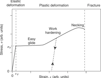
3 Mechanical Properties 33
3.1 Elastic Deformation 35
3.1.1 Macroscopic Picture 35
3.1.1.1 Elastic Constants 35
3.1.1.2 Poisson’s Ratio 36
3.1.1.3 Relation between Elastic Constants 37
3.1.2 Microscopic Picture 37
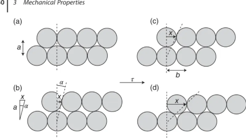
3.2 Plastic Deformation 38
3.2.1 Estimate of the Yield Stress 39
3.2.2 Point Defects and Dislocations 41
3.2.3 The Role of Defects in Plastic Deformation 41
3.3 Fracture 43
3.4 Further Reading 44
3.5 Discussion and Problems 45
4 Thermal Properties of the Lattice 47
4.1 Lattice Vibrations 47
4.1.1 A Simple Harmonic Oscillator 47
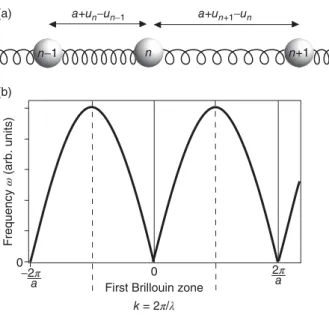
4.1.2 An Infinite Chain of Atoms 48
4.1.2.1 One Atom Per Unit Cell 48
4.1.2.2 The First Brillouin Zone 51
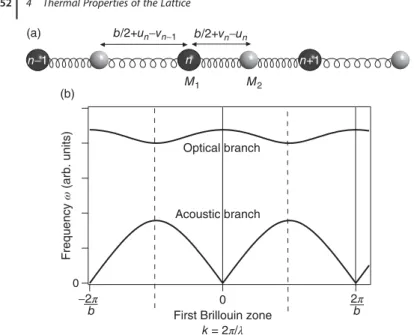
4.1.2.3 Two Atoms per Unit Cell 52
4.1.3 A Finite Chain of Atoms 53
4.1.4 Quantized Vibrations, Phonons 55
4.1.5 Three-Dimensional Solids 57
4.1.5.1 Generalization to Three Dimensions 57
4.1.5.2 Estimate of the Vibrational Frequencies from the Elastic
Constants 58
4.2 Heat Capacity of the Lattice 60
4.2.1 Classical Theory and Experimental Results 60
4.2.2 Einstein Model 62
4.2.3 Debye Model 63
4.3 Thermal Conductivity 67
4.4 Thermal Expansion 70
4.5 Allotropic Phase Transitions and Melting 71
References 74
4.6 Further Reading 74
4.7 Discussion and Problems 74
5 Electronic Properties of Metals: Classical Approach 77
5.1 Basic Assumptions of the Drude Model 77
5.2 Results from the Drude Model 79
Contents VII
5.2.1 DC Electrical Conductivity 79
5.2.2 Hall Effect 81
5.2.3 Optical Reflectivity of Metals 82
5.2.4 The Wiedemann–Franz Law 85
5.3 Shortcomings of the Drude Model 86
5.4 Further Reading 87
5.5 Discussion and Problems 87
6 Electronic Properties of Solids: Quantum Mechanical Approach 91
6.1 The Idea of Energy Bands 92
6.2 Free Electron Model 94
6.2.1 The Quantum Mechanical Eigenstates 94
6.2.2 Electronic Heat Capacity 99
6.2.3 The Wiedemann–Franz Law 100
6.2.4 Screening 101
6.3 The General Form of the Electronic States 103
6.4 Nearly Free Electron Model 106
6.5 Tight-binding Model 111
6.6 Energy Bands in Real Solids 116
6.7 Transport Properties 122
6.8 Brief Review of Some Key Ideas 126
References 127
6.9 Further Reading 127
6.10 Discussion and Problems 127
7 Semiconductors 131
7.1 Intrinsic Semiconductors 132
7.1.1 Temperature Dependence of the Carrier Density 134
7.2 Doped Semiconductors 139 7.2.1 n and p Doping 139 7.2.2 Carrier Density 141 7.3 Conductivity of Semiconductors 144 7.4 Semiconductor Devices 145 7.4.1 The pn Junction 145 7.4.2 Transistors 150 7.4.3 Optoelectronic Devices 151 7.5 Further Reading 155
7.6 Discussion and Problems 155
8 Magnetism 159
8.1 Macroscopic Description 159
8.2 Quantum Mechanical Description of Magnetism 161
8.3 Paramagnetism and Diamagnetism in Atoms 163
8.4 Weak Magnetism in Solids 166
8.4.1 Diamagnetic Contributions 167
VIII Contents
8.4.1.1 Contribution from the Atoms 167
8.4.1.2 Contribution from the Free Electrons 167
8.4.2 Paramagnetic Contributions 168
8.4.2.1 Curie Paramagnetism 168
8.4.2.2 Pauli Paramagnetism 170
8.5 Magnetic Ordering 171
8.5.1 Magnetic Ordering and the Exchange Interaction 172
8.5.2 Magnetic Ordering for Localized Spins 174
8.5.3 Magnetic Ordering in a Band Picture 178
8.5.4 Ferromagnetic Domains 180
8.5.5 Hysteresis 181
References 182
8.6 Further Reading 183
8.7 Discussion and Problems 183
9 Dielectrics 187
9.1 Macroscopic Description 187
9.2 Microscopic Polarization 189
9.3 The Local Field 191
9.4 Frequency Dependence of the Dielectric Constant 192
9.4.1 Excitation of Lattice Vibrations 192
9.4.2 Electronic Transitions 196 9.5 Other Effects 197 9.5.1 Impurities in Dielectrics 197 9.5.2 Ferroelectricity 198 9.5.3 Piezoelectricity 199 9.5.4 Dielectric Breakdown 200 9.6 Further Reading 200
9.7 Discussion and Problems 201
10 Superconductivity 203
10.1 Basic Experimental Facts 204
10.1.1 Zero Resistivity 204
10.1.2 The Meissner Effect 207
10.1.3 The Isotope Effect 209
10.2 Some Theoretical Aspects 210
10.2.1 Phenomenological Theory 210
10.2.2 Microscopic BCS Theory 212
10.3 Experimental Detection of the Gap 218
10.4 Coherence of the Superconducting State 220
10.5 Type I and Type II Superconductors 222
10.6 High-Temperature Superconductivity 224
10.7 Concluding Remarks 226
References 227
Contents IX
10.8 Further Reading 227
10.9 Discussion and Problems 227
11 Finite Solids and Nanostructures 231
11.1 Quantum Confinement 232
11.2 Surfaces and Interfaces 234
11.3 Magnetism on the Nanoscale 237
11.4 Further Reading 238
11.5 Discussion and Problems 239
Appendix A 241
A.1 Explicit Forms of Vector Operations 241
A.2 Differential Form of the Maxwell Equations 242
A.3 Maxwell Equations in Matter 243
Index 245
XI
Preface of the First Edition
This book emerged from a course on solid state physics for third-year students of physics and nanoscience, but it should also be useful for students of related fields such as chemistry and engineering. The aim is to provide a bachelor-level survey over the whole field without going into too much detail. With this in mind, a lot of emphasis is put on a didactic presentation and little on stringent mathematical derivations or completeness. For a more in-depth treatment, the reader is referred to the many excellent advanced solid state physics books. A few are listed in the Appendix.
To follow this text, a basic university-level physics course is required as well as some working knowledge of chemistry, quantum mechanics, and statistical physics. A course in classical electrodynamics is of advantage but not strictly nec-essary.
Some remarks on how to use this book: Every chapter is accompanied by a set of ”discussion” questions and problems. The intention of the questions is to give the student a tool for testing his/her understanding of the subject. Some of the ques-tions can only be answered with knowledge of later chapters. These are marked by an asterisk. Some of the problems are more of a challenge in that they are more difficult mathematically or conceptually or both. These problems are also marked by an asterisk. Not all the information necessary for solving the problems is given here. For standard data, for example, the density of gold or the atomic weight of copper, the reader is referred to the excellent resources available on the World Wide Web.
Finally, I would like to thank the people who have helped me with many discus-sions and suggestions. In particular, I would like to mention my colleagues Arne Nylandsted Larsen, Ivan Steensgaard, Maria Fuglsang Jensen, Justin Wells, and many others involved in teaching the course in Aarhus.
XIII
Preface of the Second Edition
The second edition of this book is slightly enlarged in some subject areas and significantly improved throughout. The enlargement comprises subjects that turned out to be too essential to be missing, even in a basic introduction such as this one. One example is the tight-binding model for electronic states in solids, which is now added in its simplest form. Other enlargements reflect recent developments in the field that should at least be mentioned in the text and explained on a very basic level, such as graphene and topological insulators.
I decided to support the first edition by online material for subjects that were either crucial for the understanding of this text, but not familiar to all readers, or not central enough to be included in the book but still of interest. This turned out to be a good concept, and the new edition is therefore supported by an extended number of such notes; they are referred to in the text. The notes can be found on my homepage www.philiphofmann.net.
The didactical presentation has been improved, based on the experience of many people with the first edition. The most severe changes have been made in the chapter on magnetism but minor adjustments have been made throughout the book. In these changes, didactic presentation was given a higher priority than elegance or conformity to standard notation, for example, in the figures on Pauli paramagnetism or band ferromagnetism.
Every chapter now contains a “Further Reading” section in the end. Since these sections are supposed to be independent of each other, you will find that the same books are mentioned several times.
I thank the many students and instructors who participated in the last few years’ Solid State Physics course at Aarhus University, as well as many colleagues for their criticism and suggestions. Special thanks go to NL architects for permitting me to use the flipper-bridge picture in Figure 11.3, to Justin Wells for suggesting the analogy to the topological insulators, to James Kermode for Figure 3.7, to Arne Nylandsted Larsen and Antonija Grubiši´c ˇCabo for advice on the sections on solar cells and magnetism, respectively.
XV
Physical Constants and Energy Equivalents
Planck constant h 6.6260755 × 10⁻³⁴J s 4.13566743 × 10⁻¹⁵eV s Boltzmann constant kB 1.380658 × 10⁻²³J K−1 8.617385 × 10⁻⁵eV K−1 Proton charge e 1.60217733 × 10⁻¹⁹C Bohr radius a0 5.29177 × 10⁻¹¹m Bohr magneton 𝜇B 9.2740154 × 10⁻²⁴J T−1
Avogadro number NA 6.0221367 × 10²³particles/mol
Speed of light c 2.99792458 × 10⁸m s−1
Rest mass of the electron me 9.1093897 × 10⁻³¹kg
Rest mass of the proton mp 1.6726231 × 10⁻²⁷kg
Rest mass of the neutron mn 1.6749286 × 10⁻²⁷kg
Atomic mass unit amu 1.66054 × 10⁻²⁷kg
Permeability of vacuum 𝜇0 4𝜋 × 10−7V s A−1m−1
Permittivity of vacuum 𝜖0 8.854187817 × 10⁻¹²C2J−1m−1
1 eV = 1.6021773 × 10⁻¹⁹J 1 K = 8.617385 × 10⁻⁵eV
1
1
Crystal Structures
Our general objective in this book is to understand the macroscopic properties of solids in a microscopic picture. In view of the many particles in solids, coming up with any microscopic description appears to be a daunting task. It is clearly impossible to solve the equations of motion (classical or quantum mechanical). Fortunately, it turns out that solids are often crystalline, with the atoms arranged on a regular lattice, and this symmetry permits us to solve microscopic mod-els, despite the very many particles involved. This situation is somewhat simi-lar to atomic physics where the key to a description is the spherical symmetry of the atom. We will often imagine a solid as one single crystal, a perfect lat-tice of atoms without any defects whatsoever, and it may seem that such perfect crystals are not particularly relevant for real materials. But this is not the case. Many solids are actually composed of small crystalline grains. These solids are called polycrystalline, in contrast to a macroscopic single crystal, but the num-ber of atoms in a perfect crystalline environment is still very large compared to the number of atoms on the grain boundary. For instance, for a grain size on the order of 10003atomic distances, only about 0.1% of the atoms are at the grain boundaries. There are, however, some solids that are not crystalline. These are called amorphous. The amorphous state is characterized by the absence of any long-range order. There may, however, be some short-range order between the atoms.
This chapter is divided into three parts. In the first part, we define some basic mathematical concepts needed to describe crystals. We keep things simple and mostly use two-dimensional examples to illustrate the ideas. In the second part, we discuss common crystal structures. At this point, we do not ask why the atoms bind together in the way that they do, as this is treated in the next chapter. Finally, we go into a somewhat more detailed discussion of X-ray diffraction, the experimental technique that can be used to determine the microscopic structure of crystals. X-ray diffraction is used not only in solid state physics but also for a wide range of problems in nanotechnology and structural biology.
Solid State Physics: An Introduction, Second Edition. Philip Hofmann.
© 2015 Wiley-VCH Verlag GmbH & Co. KGaA. Published 2015 by Wiley-VCH Verlag GmbH & Co. KGaA.
2 1 Crystal Structures
1.1
General Description of Crystal Structures
Our description of crystals starts with the mathematical definition of the lattice. A lattice is a set of regularly spaced points with positions defined as multiples of generating vectors. In two dimensions, a lattice can be defined as all the points that can be reached by the vectors𝐑, created from two vectors 𝐚𝟏and𝐚𝟐as
𝐑 = m𝐚𝟏+n𝐚𝟐, (1.1)
where n and m are integers. In three dimensions, the definition is
𝐑 = m𝐚𝟏+n𝐚𝟐+o𝐚𝟑. (1.2)
Such a lattice of points is also called a Bravais lattice. The number of possible Bravais lattices that differ by symmetry is limited to 5 in two dimensions and to 14 in three dimensions. An example of a two-dimensional Bravais lattice is given in Figure 1.1. The lengths of the vectors𝐚𝟏 and𝐚𝟐 are often called the lattice
constants.
Having defined the Bravais lattice, we move on to the definition of the
prim-itive unit cell. This is any volume of space that, when translated through all the
vectors of the Bravais lattice, fills space without overlap and without leaving voids. The primitive unit cell of a lattice contains only one lattice point. It is also possi-ble to define nonprimitive unit cells that contain several lattice points. These fill space without leaving voids when translated through a subset of the Bravais lattice vectors. Possible choices of a unit cell for a two-dimensional rectangular Bravais lattice are given in Figure 1.2. From the figure, it is evident that a nonprimitive unit cell has to be translated by a multiple of one (or two) lattice vectors to fill space without voids and overlap. A special choice of the primitive unit cell is the
Wigner–Seitz cell that is also shown in Figure 1.2. It is the region of space that is
closer to one given lattice point than to any other.
The last definition we need in order to describe an actual crystal is that of a basis. The basis is what we “put” on the lattice points, that is, the building block for the real crystal. The basis can consist of one or several atoms. It can even consist of
a2 a1
Figure 1.1 Example for a two-dimensional Bravais lattice.
1.1 General Description of Crystal Structures 3 Primitive unit cells Nonprimitive unit cells Wigner–Seitz cell
Figure 1.2 Illustration of unit cells (primitive and nonprimitive) and of the Wigner–Seitz cell for a rectangular two-dimensional lattice.
complex molecules as in the case of protein crystals. Different cases are illustrated in Figure 1.3.
Finally, we add a remark about symmetry. So far, we have discussed
trans-lational symmetry. But for a real crystal, there is also point symmetry.
Compare the structures in the middle and the bottom of Figure 1.3. The former structure possesses a couple of symmetry elements that the latter does not have, for example, mirror lines, a rotational axis, and inversion symmetry. The knowledge of such symmetries can be very useful for the description of crystal properties. + = + = + = Bravais lattice Basis Crystal
Figure 1.3 A two-dimensional Bravais lattice with different choices for the basis.
4 1 Crystal Structures
1.2
Some Important Crystal Structures
After this rather formal treatment, we look at a number of common crystal struc-tures for different types of solids, such as metals, ionic solids, or covalently bonded solids. In the next chapter, we will take a closer look at the details of these bonding types.
1.2.1
Cubic Structures
We start with one of the simplest possible crystal structures, the simple cubic
structure shown in Figure 1.4a. This structure is not very common among
ele-mental solids, but it is an important starting point for many other structures. The reason why it is not common is its openness, that is, that there are many voids if we think of the ions as spheres touching each other. In metals, the most common elemental solids, directional bonding is not important and a close packing of the ions is usually favored. For covalent solids, directional bonding is important but six bonds on the same atom in an octahedral configuration are not common in elemental solids.
The packing density of the cubic structure is improved in the body-centered
cubic (bcc) and face-centered cubic (fcc) structures that are also shown in
Figure 1.4. In fact, the fcc structure has the highest possible packing density for spheres as we shall see later. These two structures are very common. Seventeen elements crystallize in the bcc structure and 24 elements in the fcc structure. Note that only for the simple cubic structure, the cube is identical with the Bravais lattice. For the bcc and fcc lattices, the cube is also a unit cell, but not the primitive one. Both structures are Bravais lattices with a basis containing one atom but the vectors spanning these Bravais lattices are not the edges of the cube.
(a) Simple cubic (b) Body-centered cubic (c) Face-centered cubic
Figure 1.4 (a) Simple cubic structure; (b) body-centered cubic structure; and (c) face-centered cubic structure. Note that the spheres are depicted much smaller
than in the situation of most dense pack-ing and not all of the spheres on the faces of the cube are shown in (c).
1.2 Some Important Crystal Structures 5
CsCl structure NaCl structure
a
Cs+
CI−
Na+
CI−
Figure 1.5 Structures of CsCl and NaCl. The spheres are depicted much smaller than in the situation of most dense packing, but the relative size of the different ions in each structure is correct.
Cubic structures with a more complex basis than a single atom are also impor-tant. Figure 1.5 shows the structures of the ionic crystals CsCl and NaCl that are both cubic with a basis containing two atoms. For CsCl, the structure can be thought of as two simple cubic structures stacked into each other. For NaCl, it consists of two fcc lattices stacked into each other. Which structure is preferred for such ionic crystals depends on the relative size of the ions.
1.2.2
Close-Packed Structures
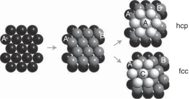
Many metals prefer structural arrangements where the atoms are packed as closely as possible. In two dimensions, the closest possible packing of ions (i.e., spheres) is the hexagonal structure shown on the left-hand side of Figure 1.6. For building a three-dimensional close-packed structure, one adds a second layer as in the middle of Figure 1.6. For adding a third layer, there are then two possibilities. One can either put the ions in the “holes” just on top of the first layer ions, or one can put them into the other type of “holes.” In this way, two different crystal structures can be built. The first has an ABABAB... stacking sequence, and the second has an ABCABCABC... stacking sequence. Both have exactly the
A A A C A hcp fcc A B B B
Figure 1.6 Close packing of spheres leading to the hcp and fcc structures.
6 1 Crystal Structures
same packing density, and the spheres fill 74% of the total volume. The former structure is called the hexagonal close-packed structure (hcp), and the latter turns out to be the fcc structure we already know. An alternative sketch of the hcp structure is shown in Figure 1.14b. The fcc and hcp structures are very common for elemental metals. Thirty-six elements crystallize as hcp and 24 elements as fcc. These structures also maximize the number of nearest neighbors for a given atom, the so-called coordination number. For both the fcc and the hcp lattice, the coordination number is 12.
An open question is why, if coordination is so important, not all metals crys-tallize in the fcc or hcp structure. A prediction of the actual structure for a given element is not possible with simple arguments. However, we can collect some fac-tors that play a role. Not optimally packed structures, such as the bcc structure, have a lower coordination number, but they bring the second-nearest neighbors much closer to a given ion than in the close-packed structures. Another important consideration is that the bonding is not quite so simple, especially for transition
metals. In these, bonding is not only achieved through the delocalized s and p
valence electrons as in simple metals, but also by the more localized d electrons. Bonding through the latter has a much more directional character, so that not only the close packing of the ions is important.
The structures of many ionic solids can also be viewed as “close-packed” in some sense. One can arrive at these structures by treating the ions as hard spheres that have to be packed as closely to each other as possible.
1.2.3
Structures of Covalently Bonded Solids
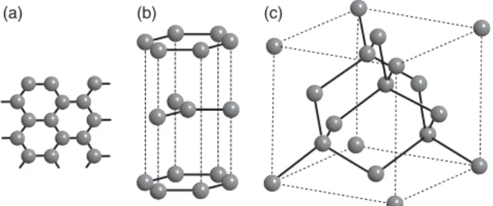
In covalent structures, the atoms’ valence electrons are not completely delocalized but shared between neighboring atoms and the bond length and direction are far more important than the packing density. Prominent examples are graphene, graphite, and diamond as displayed in Figure 1.7. Graphene is a single sheet of carbon atoms in a honeycomb lattice structure. It is a truly two-dimensional solid with a number of remarkable properties; so remarkable, in fact, that their
(b)
(a) (c)
Figure 1.7 Structures for (a) graphene, (b) graphite, and (c) diamond. sp2and sp3bonds
are displayed as solid lines.
1.3 Crystal Structure Determination 7
discovery has lead to the 2010 Nobel prize in physics being awarded to A. Geim and K. Novoselov. The carbon atoms in graphene are connected by sp2 hybrid bonds, enclosing an angle of 120∘. The parent material of graphene is graphite, a stack of graphene sheets that are weakly bonded to each other. In fact, graphene can be isolated from graphite by peeling off flakes with a piece of scotch tape. In diamond, the carbon atoms form sp3-type bonds and each atom has four nearest neighbors in a tetrahedral configuration. Interestingly, the diamond structure can also be described as an fcc Bravais lattice with a basis of two atoms.
The diamond structure is also found for Si and Ge. Many other isoelectronic materials (with the same total number of valence electrons), such as SiC, GaAs, and InP, also crystallize in a diamond-like structure but with each element on a different fcc sublattice.
1.3
Crystal Structure Determination
After having described different crystal structures, the question is of course how to determine these structures in the first place. By far, the most important technique for doing this is X-ray diffraction. In fact, the importance of this technique goes far beyond solid state physics, as it has become an essential tool for fields such as structural biology as well. There the idea is that, if you want to know the structure of a given protein, you can try to crystallize it and use the powerful methodology for structural determination by X-ray diffraction. We will also use X-ray diffraction as a motivation to extend our formal description of structures a bit.
1.3.1
X-Ray Diffraction
X-rays interact rather weakly with matter. A description of X-ray diffraction can therefore be restricted to single scattering, that is, incoming X-rays get scattered not more than once (most are not scattered at all). This is called the kinematic
approximation; it greatly simplifies matters and is used throughout the treatment
here. In addition to this, we will assume that the X-ray source and detector are very far away from the sample so that the incoming and outgoing waves can be treated as plane waves. X-ray diffraction of crystals was discovered and described by M. von Laue in 1912. Also in 1912, W. L. Bragg came up with an alternative description that is considerably simpler and serves as a starting point here.
1.3.1.1 Bragg Theory
Bragg treated the problem as the reflection of the incoming X-rays at flat crystal planes. These planes could, for example, be the close-packed planes making up the fcc and hcp crystals, or they could be alternating Cs and Cl planes making up the CsCl structure. At first glance, this has very little physical justification because the crystal planes are certainly not “flat” for X-rays that have a wavelength similar to the atomic spacing. Nevertheless, the description is highly successful, and we
8 1 Crystal Structures A B d 𝜃 𝜃 𝜃 𝜃
Figure 1.8 Construction for the derivation of the Bragg condition. The horizontal lines represent the crystal lattice planes that are separated by a distance d. The heavy lines represent the X-rays.
shall later see that it is actually a special case of the more complex Laue description of X-ray diffraction.
Figure 1.8 shows the geometrical considerations behind the Bragg description. A collimated beam of monochromatic X-rays hits the crystal. The intensity of diffracted X-rays is measured in the specular direction. The angle of incidence and emission is 90∘ − Θ. The condition for constructive interference is that the path length difference between the X-rays reflected from one layer and the next layer is an integer multiple of the wavelength𝜆. In the figure, this means that 2AB = n𝜆, where AB is the distance between points A and B and n is a natural number. On the other hand, we have sin𝜃 = AB∕d such that we arrive at the Bragg condition
n𝜆 = 2d sin 𝜃. (1.3)
It is obvious that if this condition is fulfilled for one layer and the layer below, it will also be fulfilled for any number of layers with identical spacing. In fact, the X-rays penetrate very deeply into the crystal so that thousands of layers contribute to the reflection. This results into very sharp maxima in the diffracted intensity, similar to the situation for an optical grating with many lines. The Bragg condition can obviously only be fulfilled for𝜆 < 2d, putting an upper limit on the wavelength of the X-rays that can be used for crystal structure determination.
1.3.1.2 Lattice Planes and Miller Indices
The Bragg condition will work not only for a special kind of lattice plane in a crys-tal, such as the hexagonal planes in an hcp cryscrys-tal, but for all possible parallel planes in a structure. We therefore come up with a more stringent definition of the term lattice plane. It can be defined as a plane containing at least three non-collinear points of a given Bravais lattice. If it contains three, it will actually contain infinitely many because of translational symmetry. Examples for lattice planes in a simple cubic structure are shown in Figure 1.9.
The lattice planes can be characterized by a set of three integers, the so-called
Miller indices. We arrive at these in three steps:
1) We find the intercepts of the plane with the crystallographic axes in units of the lattice vectors, for example, (1, ∞, ∞) for the leftmost plane in Figure 1.9.
1.3 Crystal Structure Determination 9 (1,0,0) (1,1,0) (1,1,1) a2 a3 a1 a3 a2 a1 a1 a2 a3
Figure 1.9 Three different lattice planes in the simple cubic structure characterized by their Miller indices.
2) We take the “reciprocal value” of these three numbers. For our example, this gives (1, 0, 0).
3) By multiplying with some factor, we reduce the numbers to the smallest set of integers having the same ratio. This is not necessary in the example as we already have integer values.
Such a set of three integers can then be used to denote any given lattice plane. Later, we will encounter a different and more elegant definition of the Miller indices.
In practice, the X-ray diffraction peaks are so sharp that it is difficult to align and move the sample such that the incoming and reflected X-rays lie in one plane with the normal direction to a certain crystal plane. An elegant way to circumvent this problem is to use a powder of very small crystals instead of a large single crystal. This will not only ensure that some small crystals are orientated correctly to get constructive interference from a certain set of crystal planes, it will automatically give the interference pattern for all possible crystal planes.
1.3.1.3 General Diffraction Theory
The Bragg theory for X-ray diffraction is useful for extracting the distances between lattice planes in a crystal, but it has its limitations. Most importantly, it does not give any information on what the lattice actually consists of, that is, the basis. Also, the fact that the X-rays should be reflected by planes is physically somewhat obscure. We now discuss a more general description of X-ray diffraction that goes back to M. von Laue.
The physical process leading to X-ray scattering is that the electromagnetic field of the X-rays forces the electrons in the material to oscillate with the same fre-quency as that of the field. The oscillating electrons then emit new X-rays that give rise to an interference pattern. For the following discussion, however, it is merely important that something scatters the X-rays, not what it is.
It is highly beneficial to use the complex notation for describing the electromagnetic X-ray waves. For the electric field, a general plane wave can be written as
(𝐫, t) = 0ei𝐤⋅𝐫−i𝜔t. (1.4)
10 1 Crystal Structures R r k′ R′ k
Figure 1.10 Illustration of X-ray scattering from a sample. The source and detector for the X-rays are placed at 𝐑 and 𝐑′, respectively. Both are very far away from the sample.
The wave vector𝐤 points in the direction of the wave propagation with a length of 2𝜋∕𝜆, where 𝜆 is the wavelength. The convention is that the physical electric field is obtained as the real part of the complex field and the intensity of the wave is obtained as
I(𝐫) = |0ei𝐤⋅𝐫−i𝜔t|2=|0|2. (1.5) Consider now the situation depicted in Figure 1.10. The source of the X-rays is far away from the sample at the position𝐑, so that the X-ray wave at the sample can be described as a plane wave. The electric field at a point𝐫 in the crystal at time t can be written as
(𝐫, t) = 0ei𝐤⋅(𝐫−𝐑)−i𝜔t. (1.6) Before we proceed, we can drop the absolute amplitude0from this expression because we are only concerned with relative phase changes. The field at point𝐫 is then
(𝐫, t) ∝ ei𝐤⋅(𝐫−𝐑)e−i𝜔t. (1.7) A small volume element dV located at𝐫 will give rise to scattered waves in all directions. The direction of interest is the direction towards the detector that shall be placed at the position𝐑′, in the direction of a second wave vector𝐤′. We assume that the amplitude of the wave scattered in this direction will be proportional to the incoming field from (1.7) and to a factor𝜌(𝐫) describing the scattering proba-bility and scattering phase. We already know that the scattering of X-rays proceeds via the electrons in the material, and for our purpose, we can view𝜌(𝐫) as the electron concentration in the solid. For the field at the detector, we obtain
(𝐑′, t) ∝ (𝐫, t)𝜌(𝐫)ei𝐤′⋅(𝐑′−𝐫)
. (1.8)
Again, we have assumed that the detector is very far away from the sample such that the scattered wave at the detector can be written as a plane wave. Inserting (1.7) gives the field at the detector as
(𝐑′, t) ∝ ei𝐤⋅(𝐫−𝐑)𝜌(𝐫)ei𝐤′⋅(𝐑′−𝐫)
e−i𝜔t=ei(𝐤′⋅𝐑′−𝐤⋅𝐑)
𝜌(𝐫)ei(𝐤−𝐤′)⋅𝐫
e−i𝜔t. (1.9)
1.3 Crystal Structure Determination 11
We drop the first factor that does not contain𝐫 and will thus not play a role for the interference of X-rays emitted from different positions in the sample. The total wave field at the detector can finally be calculated by integrating over the entire volume of the crystal V . As the detector is far away from the sample, the wave vector𝐤′is essentially the same for all points in the sample. The result is
(𝐑′, t) ∝ e−i𝜔t
∫V𝜌(𝐫)ei(𝐤−𝐤
′)⋅𝐫
dV. (1.10)
In most cases, it will only be possible to measure the intensity of the X-rays, not the field, and this intensity is
I(𝐊) ∝||||e−i𝜔t∫ V 𝜌(𝐫)ei(𝐤−𝐤′)⋅𝐫 dV|||| 2 =|| ||∫V 𝜌(𝐫)e−i𝐊⋅𝐫dV|| || 2 , (1.11)
where we have introduced the so-called scattering vector𝐊 = 𝐤′−𝐤, which is just the difference of outgoing and incoming wave vectors. Note that although the direction of the wave vector for the scattered waves𝐤′is different from that of the incoming wave𝐤, the length is the same because we only consider elastic scattering.
Equation (1.11) is the final result. It relates the measured intensity to the electron concentration in the sample. Except for very light elements, most of the electrons are located close to the ion cores and the electron concentration that scatters the X-rays is essentially identical to the geometrical arrangement of the ion cores. Hence, (1.11) can be used for the desired structural determination. To this end, one could try to measure the intensity as a function of scattering vector𝐊 and to infer the structure from the result. This is a formidable task. It is greatly simpli-fied if the specimen under investigation is a crystal with a periodic lattice. In the following, we introduce the mathematical tools that are needed to exploit the crys-talline structure in the analysis. The most important one is the so-called reciprocal lattice.
1.3.1.4 The Reciprocal Lattice
The concept of the reciprocal lattice is fundamental to solid state physics because it permits us to exploit the crystal symmetry for the analysis of many problems. Here we will use it to describe X-ray diffraction from periodic structures and we will meet it again and again in the next chapters. Unfortunately, the meaning of the reciprocal lattice turns out to be hard to grasp. Here, we choose to start out with a formal definition and we provide some mathematical properties. We then discuss the meaning of the reciprocal lattice before we come back to X-ray diffraction. The full importance of the concept will become apparent throughout this book.
For a given Bravais lattice
𝐑 = m𝐚𝟏+n𝐚𝟐+o𝐚𝟑, (1.12) we define the reciprocal lattice as the set of vectors𝐆 for which
𝐑 ⋅ 𝐆 = 2𝜋l, (1.13)
12 1 Crystal Structures
where l is an integer. Equivalently, we could require that
e𝐢𝐆⋅𝐑=1. (1.14)
Note that this equation must hold for any choice of the lattice vector𝐑 and recip-rocal lattice vector𝐆. We can write any 𝐆 as the sum of three vectors
𝐆 = m′𝐛
𝟏+n′𝐛𝟐+o′𝐛𝟑, (1.15)
where m′, n′and o′are integers. The reciprocal lattice is again a Bravais lattice. The vectors𝐛𝟏,𝐛𝟐, and𝐛𝟑spanning the reciprocal lattice can be constructed explicitly from the lattice vectors
𝐛1=2𝜋 𝐚2×𝐚3 𝐚1⋅ (𝐚2×𝐚3) , 𝐛2=2𝜋 𝐚3×𝐚1 𝐚1⋅ (𝐚2×𝐚3) , 𝐛3=2𝜋 𝐚1×𝐚2 𝐚1⋅ (𝐚2×𝐚3) . (1.16) From this, one can derive the simple but useful property,1)
𝐚i⋅ 𝐛j=2𝜋𝛿ij, (1.17)
which can easily be verified. Equation (1.17) can then be used to verify that the reciprocal lattice vectors defined by (1.15) and (1.16) do indeed fulfill the funda-mental property of (1.13) that defines the reciprocal lattice (see Problem 1.6).
Another way to view the vectors of the reciprocal lattice is as wave vectors that yield plane waves with the periodicity of the Bravais lattice because
ei𝐆⋅𝐫=ei𝐆⋅𝐫ei𝐆⋅𝐑=ei𝐆⋅(𝐫+𝐑). (1.18)
Finally, one can define the Miller indices in a much simpler way using the recip-rocal lattice: The Miller indices (i, j, k) define a plane that is perpendicular to the reciprocal lattice vector i𝐛𝟏+j𝐛𝟐+k𝐛𝟑(see Problem 1.8).
1.3.1.5 The Meaning of the Reciprocal Lattice
We have now defined the reciprocal lattice in a proper way, and we will give some simple examples of its usefulness. The most important point of the reciprocal lat-tice is that it facilitates the description of functions that have the periodicity of the lattice. To see this, consider a one-dimensional lattice, a chain of points with a lat-tice constant a. We are interested in a function with the periodicity of the latlat-tice, like the electron concentration along the chain𝜌(x) = 𝜌(x + a). We can write this as a Fourier series of the form
𝜌(x) = C +
∞ ∑ n=1
{
Cncos(x2𝜋n∕a) + Snsin(x2𝜋n∕a) }
(1.19) with real coefficients Cnand Sn. The sum starts at n = 1, that is, the constant part
C has to be taken out of the sum. We can also write this in a more compact form 𝜌(x) =
∞ ∑ n=−∞
𝜌neixn2𝜋∕a, (1.20)
1)𝛿ijis Kronecker’s delta, which is 1 for i = j and zero otherwise.
1.3 Crystal Structure Determination 13 3 2 1 0 −5 −2.5 0 2.5 5 a 3 2 1 0 0 −5 5
Real space Reciprocal space
4 2 0 3 2 1 0 n 2π/a ρ( x ) ρ( x ) −5 −2.5 0 2.5 5 x (a) |ρn | |ρn | 0 −5 5
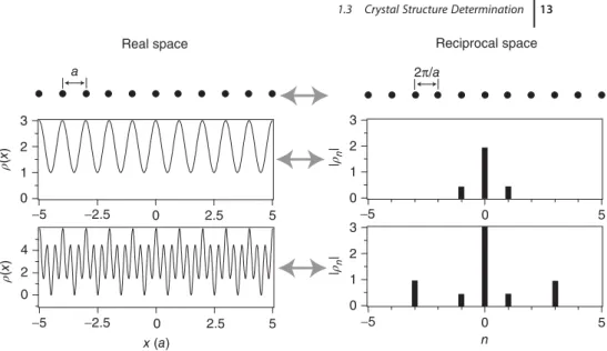
Figure 1.11 Top: Chain with a lattice con-stant a as well as its reciprocal lattice, a chain with a spacing of 2𝜋∕a. Middle and bottom: Two lattice-periodic functions 𝜌(x)
in real space as well as their Fourier cients. The magnitude of the Fourier coeffi-cients |𝜌n| is plotted on the reciprocal lattice
vectors they belong to.
using complex coefficients𝜌n. To ensure that𝜌(x) is still a real function, we have to require that
𝜌∗
−n =𝜌n, (1.21)
that is, that the coefficient𝜌−nmust be the conjugate complex of the coefficient𝜌n. This description is more elegant than the one with the sine and cosine functions. How is it related to the reciprocal lattice? In one dimension, the reciprocal lattice of a chain of points with lattice constant a is also a chain of points with spacing 2𝜋∕a (see (1.17)). This means that we can write a general reciprocal lattice “vector” as
g = n2𝜋
a , (1.22)
where n is an integer. Exactly these reciprocal lattice “vectors” appear in (1.20). In fact, (1.20) is a sum of functions with a periodicity corresponding to the recip-rocal lattice vectors, weighted by the coefficients𝜌n. Figure 1.11 illustrates these ideas by showing the lattice and reciprocal lattice for such a chain as well as two lattice-periodic functions, as real space functions and as Fourier coefficients on the reciprocal lattice points. The advantage of describing the functions by the coef-ficients𝜌nis immediately obvious: Instead of giving𝜌(x) for every point in a range of 0⩽ x < a, the Fourier description consists only of three numbers for the upper function and five numbers for the lower function. Actually, it is only two and three numbers because of (1.21).
The same ideas also work in three dimensions. In fact, one can use a Fourier sum for lattice-periodic properties, which exactly corresponds to (1.20). For the
14 1 Crystal Structures
lattice-periodic electron concentration𝜌(𝐫) = 𝜌(𝐫 + 𝐑), we get
𝜌(𝐫) =∑
𝐆
𝜌𝐆ei𝐆⋅𝐫, (1.23)
where𝐆 are the reciprocal lattice vectors.
With this we have seen that the reciprocal lattice is very useful for describing lattice-periodic functions. But this is not all: It can also simplify the treatment of waves in crystals in a very general sense. Such waves can be X-rays, elastic lattice distortions, or even electronic wave functions. We will come back to this point at a later stage.
1.3.1.6 X-Ray Diffraction from Periodic Structures
Turning back to the specific problem of X-ray diffraction, we can now exploit the fact that the electron concentration is lattice-periodic by inserting (1.23) in our expression (1.11) for the diffracted intensity. This gives
I(𝐊) ∝|||| | ∑ 𝐆 𝜌𝐆∫ V ei(𝐆−𝐊)⋅𝐫dV|||| | 2 . (1.24)
Let us inspect the integrand. The exponential function represents a plane wave with a wave vector𝐆 − 𝐊. If the crystal is very big, the integration will average over the crests and troughs of this wave and the result of the integration will be very small (or zero for an infinitely large crystal). The only exception to this is the case where
𝐊 = 𝐤′−𝐤 = 𝐆,
(1.25) that is, when the difference between incoming and scattered wave vector is equal to a reciprocal lattice vector. In this case, the exponential function in the integral is 1, and the value of the integral is equal to the volume of the crystal. Equation (1.25) is often called the Laue condition. It is central to the description of X-ray diffrac-tion from crystals in that it describes the condidiffrac-tion for the observadiffrac-tion of con-structive interference.
Looking back at (1.24), the observation of constructive interference for a chosen scattering geometry (or scattering vector𝐊) clearly corresponds to a particular reciprocal lattice vector𝐆. The intensity measured at the detector is proportional to the square of the Fourier coefficient of the electron concentration|𝜌𝐆|2. We could therefore think of measuring the intensity of the diffraction spots appearing for all possible reciprocal lattice vectors, obtaining the Fourier coefficients of the electron concentration and reconstructing this concentration. This would give all the information needed and conclude the process of the structural determination. Unfortunately, this straightforward approach does not work because the Fourier coefficients are complex, not real numbers. Taking the square root of the inten-sity at the diffraction spot therefore gives the magnitude but not the phase of𝜌𝐆. The phase is lost in the measurement. This is known as the phase problem in X-ray diffraction. One has to work around it to solve the structure. One simple approach is to calculate the electron concentration for a structural model, obtain
1.3 Crystal Structure Determination 15
the magnitude of the𝜌𝐆values and thus also the expected diffracted intensity, and compare this to the experimental result. Based on the outcome, the model can be refined until the agreement is satisfactory.
More precisely, this can be done in the following way. We start with (1.11), the expression for the diffracted intensity that we had obtained before introducing the reciprocal lattice. But now we know that constructive interference is only observed in a geometry that corresponds to fulfilling the Laue condition and we can there-fore write the intensity for a particular diffraction spot as
I(𝐆) ∝||||∫ V 𝜌(𝐫)e−i𝐆⋅𝐫dV|| || 2 . (1.26)
We also know that the crystal is made of many identical unit cells at the positions of the Bravais lattice𝐑. We can split the integral up as a sum of integrals over the individual unit cells
I(𝐆) ∝|||| | ∑ 𝐑 ∫Vcell 𝜌(𝐫 + 𝐑)e−i𝐆⋅(𝐫+𝐑)dV|| || | 2 =|||| |N ∫Vcell 𝜌(𝐫)e−i𝐆⋅𝐫dV|| || | 2 , (1.27) where N is the number of unit cells in the crystal and we have used the lattice periodicity of𝜌(𝐫) and (1.14) in the last step. We now assume that the electron concentration in the unit cell𝜌(𝐫) is given by the sum of atomic electron concen-trations𝜌i(𝐫) that can be calculated from the atomic wave functions. By doing so, we neglect the fact that some of the electrons form the bonds between the atoms and are not part of the spherical electron cloud around the atom any longer. If the atoms are not too light, however, the number of these valence electrons is small compared to the total number of electrons and the approximation is appropriate. We can then write
𝜌(𝐫) =∑ i
𝜌i(𝐫 − 𝐫i), (1.28) where we sum over the different atoms in the unit cell at positions𝐫i. This permits us to rewrite the integral in (1.27) as a sum of integrals over the individual atoms in the unit cell
∫Vcell𝜌(𝐫)e−i𝐆⋅𝐫dV = ∑ i e−i𝐆⋅𝐫i ∫Vatom𝜌i(𝐫′)e−i𝐆⋅𝐫 ′ dV′, (1.29) where𝐫′ =𝐫 − 𝐫
i. The two exponential functions give rise to two types of inter-ference. The first describes the interference between the X-rays scattered by the different atoms in the unit cell, and the second the interference between the X-rays scattered by the electrons within one atom. The last integral is called the atomic
form factor and can be calculated from the atomic properties alone. We therefore
see how the diffracted intensity for an assumed structure can be calculated from the atomic form factors and the arrangement of the atoms.
1.3.1.7 The Ewald Construction
In 1913, P. Ewald published an intuitive geometrical construction to visualize the Laue condition (1.25) and to determine the directions𝐤′for which constructive
16 1 Crystal Structures
k′′
G
k
Figure 1.12 Ewald construction for finding the directions in which constructive interfer-ence can be observed. The dots represent the reciprocal lattice. The arrows labeled 𝐤 and 𝐤′
are the wave vectors of the incoming and scattered X-rays, respectively.
interference is to be expected. The construction is shown in Figure 1.12, which represents a cut through the reciprocal lattice; the black points are the reciprocal lattice points. The construction works as follows:
1) We draw the wave vector𝐤 of the incoming X-rays such that it ends in the origin of the reciprocal lattice (we may of course choose the point of origin freely).
2) We construct a circle of radius|𝐤| around the starting point of 𝐤.
3) Wherever the circle touches a reciprocal lattice point, the Laue condition
𝐤′−𝐤 = 𝐆 is fulfilled.
For a three-dimensional crystal, this construction has to be carried out in different planes, of course. The figure clearly shows that (1.25) is a very stringent condition: It is not likely for the sphere to hit a second reciprocal lattice point, so that con-structive interference is only expected for very few directions. As in the Bragg description, we see that the wavelength of the X-rays has to be short enough (|𝐤| has to be long enough) for any constructive interference to occur.
Practical X-ray diffraction experiments are often carried out in such a way that many constructive interference maxima are observed despite the strong restric-tions imposed by the Laue condition (1.25). This can, for example, be achieved by using a wide range of X-ray wavelengths, that is, non monochromatic radiation or by doing diffraction experiments not on one single crystal but on a powder of randomly oriented small crystals.
1.3.1.8 Relation Between Bragg and Laue Theory
We conclude our treatment of X-ray diffraction by showing that the Bragg descrip-tion of X-ray diffracdescrip-tion is just a special case of the Laue descripdescrip-tion. We start by noting that the Laue condition (1.25) consists, in fact, of three separate conditions for the three components of the vectors. In the Bragg experiment, two of these
1.3 Crystal Structure Determination 17
conditions are automatically fulfilled because of the specular geometry: The wave vector change parallel to the lattice planes is zero. So, the vector equation (1.25) reduces to the scalar equation
k′⟂−k⟂=2k⟂=22𝜋
𝜆 sin Θ = G⟂, (1.30)
where G⟂ is a reciprocal lattice vector perpendicular to the lattice planes. We have seen in Section 1.3.1.4 that such a reciprocal lattice vector exists for any set of planes. The planes can be defined by their Miller indices (i, j, k) or by the reciprocal lattice vector𝐆⟂=i𝐛𝟏+j𝐛𝟐+k𝐛𝟑that is perpendicular to the planes (see Problem 1.8). The shortest possible𝐆⟂has a length of 2𝜋∕d with d being the distance between the planes, but any integer multiple of this will also work. If we thus insert m2𝜋∕d for G⟂into (1.30), we obtain the usual form of the Bragg condition (1.3).
1.3.2
Other Methods for Structural Determination
While X-ray diffraction is arguably the most widespread and powerful method for structural determination, other techniques are used as well. Similar diffraction experiments can be carried out by making use of the wave character of neutrons or electrons. The former interact very weakly with matter because they are charge-neutral. They are also more difficult to produce than X-rays. However, the use of neutrons has two distinct advantages over X-rays: First, that their relative interac-tion strength with light atoms is stronger and second, that they carry a magnetic moment. They can therefore interact with the magnetic moments in the solid, that is, one can determine the magnetic order. Electrons, on the other hand, have the advantages that they are easy to produce and that one can use electron-optical imaging techniques, whereas making optical elements for X-rays is very difficult. On the other hand, their very strong interaction with matter causes a breakdown of the kinematic approximation, that is, multiple scattering events have to be taken into account. Because of the strong interaction with matter, low-energy electrons do not penetrate deeply into crystals either. Therefore, they are more appropriate for surface structure determination.
1.3.3
Inelastic Scattering
Our discussion has been confined to the case of elastic scattering. In real experi-ments, however, the X-rays or particles can also lose energy during the scattering events. This can be described formally by considering the diffraction from a struc-ture that does not consist of ions at fixed positions but is time-dependent, that is, which fluctuates with the frequencies of the atomic vibrations. We cannot go into the details of inelastic scattering processes here, but it is important to emphasize that the inelastic scattering, especially of neutrons, can be used to measure the vibrational properties of a lattice.
18 1 Crystal Structures
1.4
Further Reading
The concepts of lattice-periodic solids, crystal structure, and X-ray diffraction are discussed in all standard texts on solid state physics, for example,
• Ashcroft, N.W. and Mermin, N.D. (1976) Solid State Physics, Holt-Saunders.
• Ibach, H. and Lüth, H. (2009) Solid State Physics, 4th edn, Springer.
• Kittel, C. (2005) Introduction to Solid State Physics, 8th edn, John Wiley & Sons, Inc.
• Rosenberg, H.M. (1988) The Solid State, 3rd edn, Oxford University Press. For a more detailed discussion of X-ray diffraction, see, for example,
• Als-Nielsen, J. and McMorrow, D. (2011) Elements of Modern X-Ray Physics, 2nd edn, John Wiley & Sons, Ltd.
1.5
Discussion and Problems Discussion
1) What mathematical concepts do you need to describe the structure of any crystal?
2) What are typical crystal structures for metals and why?
3) Why do covalent crystals typically have a much lower packing density than metal crystals?
4) How can the reciprocal lattice conveniently be used to describe lattice-periodic functions?
5) How can you determine the structure of crystals?
6) What is the difference between the Bragg and von Laue descriptions of X-ray diffraction?
7) How can you use the reciprocal lattice of a crystal to predict the pattern of diffracted X-rays?
Problems
1) Fundamental concepts: In the two-dimensional crystal in Figure 1.13, find (a)
the Bravais lattice and a primitive unit cell, (b) a nonprimitive, rectangular unit cell, and (c) the basis.
2) Real crystal structures: Show that the packing of spheres in a simple cubic
lattice fills 52% of available space.
3) Real crystal structures: Figure 1.14 shows the structure for a two-dimensional
hexagonal packed layer of atoms, a hcp crystal, a two-dimensional sheet of carbon atoms arranged in a honeycomb lattice (graphene), and three-dimensional graphite. (a) Draw a choice of vectors spanning the Bravais
1.5 Discussion and Problems 19
Figure 1.13 A two-dimensional crystal.
c a (b) (a) (d) (c)
Figure 1.14 (a) Two-dimensional crys-tal structure of a hexagonal close-packed layer of atoms. (b) Crystal structure for a three-dimensional hcp crystal. (c) Two-dimensional crystal structure for graphene.
(d) Three-dimensional crystal structure for graphite (strongly compressed along the c direction). The lines are a mere guide to the eye, not indicating bonds or the size of the unit cell.
lattice for the hexagonal layer of atoms and for graphene, and compare them to each other. (b) Show that the basis for the hexagonal layer contains one atom, while the bases for graphene and the three-dimensional hcp crystal contain two atoms. (c) (*) Choose the vectors for the Bravais lattice for graphite and show that the basis contains four atoms.
20 1 Crystal Structures
4) Real crystal structures: Consider the hcp lattice shown in Figure 1.14b. The
Bravais lattice underlying the hcp structure is given by two vectors of length
a in one plane, with an angle of 60∘ between them and a third vector of length c perpendicular to that plane. There are two atoms per unit cell. (a) Show that
for the ideal packing of spheres, the ratio c∕a = (8∕3)1∕2. (b) (*) Construct the reciprocal lattice. Does the fact that there are two atoms per unit cell in the hcp crystal have any relevance? Hint: Use the result of Problem 1.7.
5) X-ray diffraction: (a) Determine the maximum wavelength for which
con-structive interference can be observed in the Bragg model for a simple cubic crystal with a lattice constant of 3.6 Å. (b) What is the energy of the X-rays in electron volts? (c) If you were to perform neutron diffraction, what would the energy of the neutrons have to be in order to obtain the same de Broglie wave-length? (d) You could argue that if you take X-rays with twice the wavelength, you would still get a Bragg peak because there would be constructive inter-ference between the X-rays that are reflected from every other plane. Why is this argument not valid? (e) You could describe the same crystal by using a unit cell that is a bigger cube of twice the side length, containing eight atoms instead of one. The lattice constant would then be 7.2 Å. Discuss how this different description would affect the X-ray diffraction from the crystal. 6) The reciprocal lattice: Using the explicit definition of the reciprocal lattice
(1.16), show first that (1.17) is fulfilled and then, using this relation, show that the reciprocal lattice defined by (1.16) does indeed fulfill the condition (1.13). 7) The reciprocal lattice: For a two-dimensional Bravais lattice
𝐑 = m𝐚𝟏+n𝐚𝟐, (1.31) the reciprocal lattice is also two-dimensional:
𝐆 = m′𝐛
𝟏+n′𝐛𝟐. (1.32)
Often, the most practical way to construct the reciprocal lattice is to use the relation
𝐚i⋅ 𝐛j=2𝜋𝛿ij, (1.33)
which remains valid in the two-dimensional case. Find the reciprocal lattice for the three cases given in Figure 1.15.
γ Square γ Rectangular Hexagonal γ a2 a2 a2 a1 a1 a1 |a1| = |a2| |a1| ≠ |a2| |a1| = |a2| γ = 90° γ = 90° γ = 60°
Figure 1.15 Two-dimensional Bravais lattices.
1.5 Discussion and Problems 21
8) Miller indices: We have stated that the reciprocal lattice vector m𝐛𝟏+n𝐛𝟐+
o𝐛𝟑is perpendicular to the lattice plane given by the Miller indices (m, n, o). (a) Verify that this is correct for the lattice planes drawn in Figure 1.9. (b) (*) Show that this is true in general.
23
2
Bonding in Solids
After studying the structure of crystals, we now discuss the different mechanisms that lead to bonding between atoms such that they form these structures. We will encounter different scenarios such as ionic, covalent, or metallic bonding. It has to be kept in mind that these are just idealized limiting cases. Often mixed bonding types are found, for example, a combination of metallic and covalent bonding in the transition metals.
As in conventional chemistry, only a fraction of the electrons, the so-called
valence electrons, participate in the bonding. These are the electrons in the
out-ermost shell(s) of an atom. The electrons in the inner shells, or core electrons, are bound so tightly to the nucleus that their energies and wave functions are hardly influenced by the presence of other atoms in their neighborhood.
2.1
Attractive and Repulsive Forces
Two different forces must be present to establish bonding in a solid or in a mole-cule. An attractive force is necessary for any bonding. Different types of attractive forces are discussed in the following sections. A repulsive force, on the other hand, is required in order to keep the atoms from getting too close to each other. A simple expression for an interatomic potential can thus be written as
𝜙(r) = A rn −
B
rm, (2.1)
where r is the distance between the atoms and n> m, that is, the repulsive part has to prevail for short distances (sometimes, this is achieved by assuming an expo-nential repulsion potential). Such a potential and the resulting force are shown in Figure 2.1. The reason for the strong repulsion at short distances is the Pauli exclu-sion principle. For a strong overlap of the electron clouds of two atoms, the wave functions have to change in order to become orthogonal to each other, because the Pauli principle forbids having more than two electrons in the same quantum state. The orthogonalization costs much energy, hence the strong repulsion. Solid State Physics: An Introduction, Second Edition. Philip Hofmann.
© 2015 Wiley-VCH Verlag GmbH & Co. KGaA. Published 2015 by Wiley-VCH Verlag GmbH & Co. KGaA.