HAL Id: hal-00297460
https://hal.archives-ouvertes.fr/hal-00297460
Submitted on 22 May 2008
HAL is a multi-disciplinary open access
archive for the deposit and dissemination of
sci-entific research documents, whether they are
pub-lished or not. The documents may come from
teaching and research institutions in France or
abroad, or from public or private research centers.
L’archive ouverte pluridisciplinaire HAL, est
destinée au dépôt et à la diffusion de documents
scientifiques de niveau recherche, publiés ou non,
émanant des établissements d’enseignement et de
recherche français ou étrangers, des laboratoires
publics ou privés.
Influence of meteorological input data on backtrajectory
cluster analysis ? a seven-year study for southeastern
Spain
M. Cabello, J. A. G. Orza, V. Galiano, G. Ruiz
To cite this version:
M. Cabello, J. A. G. Orza, V. Galiano, G. Ruiz. Influence of meteorological input data on
backtrajec-tory cluster analysis ? a seven-year study for southeastern Spain. Advances in Science and Research,
Copernicus Publications, 2008, 2, pp.65-70. �hal-00297460�
Adv. Sci. Res., 2, 65–70, 2008 www.adv-sci-res.net/2/65/2008/
©Author(s) 2008. This work is distributed under the Creative Commons Attribution 3.0 License.
Advances in
Science and
Research
EMS
Annual
Meeting
and
8th
Eur
opean
Confer
ence
on
Applications
of
Meteor
olo
gy
2007
Influence of meteorological input data on backtrajectory
cluster analysis – a seven-year study for southeastern
Spain
M. Cabello, J. A. G. Orza, V. Galiano, and G. Ruiz
SCOLAb, F´ısica Aplicada, Universidad Miguel Hern´andez, Elche, Spain
Received: 8 January 2008 – Revised: 21 April 2008 – Accepted: 20 May 2008 – Published: 22 May 2008
Abstract. Backtrajectory differences and clustering sensitivity to the meteorological input data are studied.
Trajectories arriving in Southeast Spain (Elche), at 3000, 1500 and 500 m for the 7-year period 2000–2006 have been computed employing two widely used meteorological data sets: the NCEP/NCAR Reanalysis and the FNL data sets. Differences between trajectories grow linearly at least up to 48 h, showing faster growing after 72 h. A k-means cluster analysis performed on each set of trajectories shows differences in the identified clusters (main flows), partially because the number of clusters of each clustering solution differs for the trajec-tories arriving at 3000 and 1500 m. Trajectory membership to the identified flows is in general more sensitive to the input meteorological data than to the initial selection of cluster centroids.
1 Introduction
Backtrajectory analysis is a commonly used method to iden-tify atmospheric transport patterns and/or determine the ori-gin and pathway of air trace substances (e.g., Dorling et al., 1992; Brankov et al., 1998; Stohl et al., 2002; Jorba et al., 2004; Salvador et al., 2004).
Trajectory models are sensitive to a variety of parameters, including the source of wind field data, wind field spatial resolution, trajectory type (kinematic, isentropic, isosigma, isobaric) and the numerical integration scheme (for a review, see Stohl, 1998, and references therein). Differences bet-ween trajectories have been computed with Euclidean (EU) distances to study error sources (Rolph and Draxler, 1990; Stohl et al., 1995) and to study the sensitivity to the meteo-rological input data set (Harris et al., 2005). In this paper we report trajectory differences by computing great-circle (GC) and EU distances, and study the influence of the meteorolo-gical data on the results of backtrajectory cluster analysis.
While errors in trajectory calculation on the order of 20% of the distance travelled are considered typical (Stohl, 1998), the statistical analysis of a large number of trajectories arri-ving at a study site over a relatively long period of time in-creases the accuracy of the trajectory analysis. Therefore,
Correspondence to: J. A. G. Orza
backtrajectory cluster analysis is a suitable technique to clas-sify the air masses arriving at a study site.
Cluster analysis is a multivariate statistical technique de-signed to classify a large data set into non-predefined do-minant groups called clusters. However, clustering involves some subjective non-trivial decisions: the number of clusters to use, the selection of centroids in the initialization stage, etc. To determine the appropriate number of clusters and handle the sensitivity of the method to the initial centroids selection we have followed the procedures described by Dor-ling et al. (1992) and Mattis (2001) and considered some modifications to them in order to obtain smaller (better) va-lues of the total Root Mean Square Deviation (RMSD), the clustering figure of merit.
2 Methodology
96-h backward air trajectories arriving at 12:00 UTC in Elche (38.3◦N, 0.7◦W) for the period 2000–2006 were computed
using the HYbrid Single Particle Lagrangian Integrated Tra-jectory (HYSPLIT) model v.4 (Draxler and Rolph, 2003) with two different meteorological data sets available at the Air Resources Laboratory of the National Oceanic and At-mospheric Administration: (a) Data from the National Cen-ters for Environmental Prediction/National Center for At-mospheric Research (NCEP/NCAR) Global Reanalysis on a 2.5◦latitude-longitude grid and 17 pressure levels (RP data
66 M. Cabello et al.: Influence of meteorological input data on backtrajectory clustering hours 0 250 500 750 1000 1250 dist (km) 24 0 48 72 96 hours 0 5 10 15 20 0 24 48 72 96 3000 m mean median
(c)
0 20 40 60 80 100 0 0.02 0.04 0.06 3000 m(d)
after 96 hours quadratic fit 3000 m 1500 m 500 m great - circle Euclidean hours 24 0 48 72 96(b)
HTD (km ) 0 400 800 1200 3000 m mean median(a)
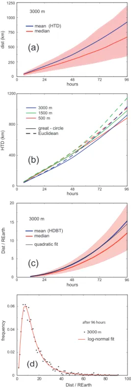
Dist / REarth log-normal fit frequency Dist / REarth (HDBT) (HTD)Figure 1. (a) Evolution of the mean, median and 25th and 75th
quartiles of the set of distnvalues computed with GC distances for trajectories arriving at 3000 m. (b) Evolution of HTD at the 3 al-titudes with the 2 distance measures. (c) Evolution of the mean, median and 25th and 75th quartiles of the Distn values computed with GC distances for trajectories arriving at 3000 m. (d) Density distribution of Distn at 96 h for the trajectories arriving at 3000 m using the GC distance.
of NCEP operational model runs (FNL data), converted from a 1◦ latitude-longitude grid and 13 pressure levels (Draxler
and Rolph, 2003). Three-dimensional trajectories that use the vertical wind component of the data set were considered. The statistical measures of trajectory sensitivity employed are closely related to those used in earlier studies (Rolph and Draxler, 1990; Stohl et al., 1995; Harris et al., 2005). The Horizontal Transport Deviation (HTD) t hours out is investi-gated by analyzing the frequency distribution of distn(t), the (GC or EU) distance between the two points corresponding to t hours of the nth pair of trajectories (FNL, RP) to com-pare. Then, for example, the HTD t hours out is the mean
HTD(t)=1 N N X n=1 distn(t), (1)
where N is the number of trajectory pairs to compare. This is identical, when computing Euclidean (latitude, longitude) distances, to the Absolute Horizontal Trajectory Deviation (AHTD) used in the literature. The great-circle distance bet-ween two points is the shortest distance in spherical geome-try; it was calculated using the haversine formula. An avera-ge Earth radius of 6731 km is used to convert GC distances from degrees to km. We have also considered the Horizontal Deviation Between Trajectories (HDBT) after t hours as the mean of the accumulated distance, Distn(t), between points of the trajectories being compared up to t hours
HDBT(t)=1 N N X n=1 Distn(t), Distn(t)= Z H 0 distn(t) dt (2)
with H the time interval between the starting and ending points of the trajectories. Calculation of Distn(t) is performed in practice as a summation that will depend on the number of points used along the trajectories; therefore some care should be taken when comparing this accumulated measure to other studies, as both hourly and 6-h trajectories are commonly found in the literature. As long as all trajectories have the same number of points, HDBT can be computed by summing the HTD values up to hour t.
The classification of the FNL and the RP trajectory sets was performed by k-means cluster analysis. Hourly latitude and longitude were used as input variables in the clustering procedures. We have followed the method described by Dor-ling et al. (1992) to reduce the subjectivity in the selection of the appropriate number of clusters: the algorithm was run for a range of cluster numbers between 30 and 2, and the per-centage change in the total RMSD (i.e. the sum of the RMSD of each cluster) when the number of clusters is reduced from
k to k−1 was used to find out the proper number of
clus-ters. When this percentage change is large (Dorling et al., 1992) or exceeds some predefined value, e.g. 5% (Brankov et al., 1998; Jorba et al., 2004), k is selected as the appro-priate number of clusters. We retain the smallest number of clusters k for which the smallest total RMSD change is found
65W 45W 25W 5W 15E 85W 60N 20N 40N 3000 m FNL RP 65W 45W 25W 5W 15E 85W 1500 m FNL RP 65W 45W 25W 5W 15E 85W 500 m FNL RP 6 clusters 7 clusters 5 clusters 6 clusters 6 clusters 6 clusters NWmod NWfast NWslow W SW SWslow MedR NWmod NWslow W SW WR MedR Med MedR NEU NWslow NWmod WR
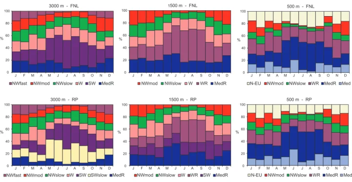
Figure 2.Final centroids (cluster means) for the trajectories arriving at 3000 m (left), 1500 m (center) and 500 m (right) for the 7-year study period computed with the FNL and the NCEP/NCAR reanalysis (RP) data.
NWfast NWmod NWslow W SW MedR
0 20 40 60 80 100 J F M A M J J A S O N D % 3000 m - FNL
NWmod NWslow W WR MedR
0 20 40 60 80 100 % 1500 m - FNL J F M A M J J A S O N D
N-EU NWmod NWslow WR MedR Med
0 20 40 60 80 100 % 500 m - FNL J F M A M J J A S O N D
NWfast NWmod NWslow W SW SWslow MedR
0 20 40 60 80 100 % 3000 m - RP J F M A M J J A S O N D
NWmod NWslow W WR SW MedR
0 20 40 60 80 100 % 1500 m - RP J F M A M J J A S O N D
N-EU NWmod NWslow WR MedR Med 500 m - RP J F M A M J J A S O N D 0 20 40 60 80 100 %
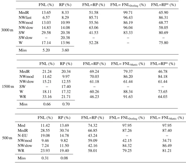
Figure 3.Seasonal variation of the frequency of the identified air mass types for the trajectory sets computed with the FNL and the RP data.
when decreasing from k+1 to k; that means that it is possible to reduce by one the number of clusters with small worsening in the total RMSD.
With respect to the way of reducing clusters from k to k−1, and the way of dealing with the dependence of the final clus-ter solution on the initial centroids, different approaches have been considered. The details of the clustering methodology we have followed and its comparison with the procedures of Dorling et al. (1992) and Mattis (2001) will be published elsewhere. Here we note that the computation of 100 000 clustering analyses for each k made independently from the previous k+1 clustering, with initial cluster centroids taken from randomly chosen real trajectories, provides smaller to-tal RMSDs and hence better clustering solutions than the ap-proaches usually found in the literature. We have considered as best solution for each k the one with the smallest RMSD.
3 Results and discussion
Figure 1 shows how the differences grow over time along the trajectories. Differences grow linearly at least up to 48 h, showing faster growing around 72 h in all cases. The distri-bution of the differences is strongly skewed. The horizontal transport deviation (HTD) at 96 h is 20% smaller than that found by Harris et al. (2005) in their comparison between tra-jectories computed with the ERA-40 and the NCEP/NCAR reanalysis data. Trajectory differences exhibit similar growth behavior using EU and GC distances (Fig. 1b) as most of the trajectories arriving at the study site remain in mid latitudes, though larger differences are found when computing EU dis-tances. The use of the GC distance is more appropriate when trajectories pass over high latitudes so this distance metric should be preferred. The highest differences are found in both cases for trajectories arriving at 1500 m: on one hand,
68 M. Cabello et al.: Influence of meteorological input data on backtrajectory clustering
Table 1.Percentage of daily trajectories classified into each air flow type for each trajectory set (columns FNL and RP) where Miss stands for days when trajectories were not available for the cluster analysis. Percentage of trajectories that fall in the same type of air flow both in FNL and RP trajectories (column FNL=RP). Percentage of days classified in the same type of air flow for the FNL trajectories when considering different clustering procedures (columns FNL= FNLDorling, FNL= FNLMattis). Percentage of trajectories classified into the same
type of air flow considering the results for the same number of clusters both for FNL and RP trajectories (column FNL=RP*).
3000 m FNL (%) RP (%) FNL=RP (%) FNL= FNLDorling(%) FNL=RP* (%) MedR 13.65 8.33 51.58 99.71 65.90 NWfast 6.57 8.29 85.71 96.43 86.31 NWmod 13.03 10.99 55.56 86.19 68.77 NWslow 14.83 14.08 63.06 96.04 58.05 SW 29.58 20.38 41.53 83.33 80.69 SWslow − 20.38 − − − W 17.14 13.96 52.28 − 75.80 Miss 5.20 3.60 1500 m FNL (%) RP (%) FNL=RP (%) FNL= FNLMattis(%) FNL=RP* (%) MedR 21.24 20.34 69.24 79.37 46.78 NWmod 11.62 9.97 70.03 86.20 84.18 NWslow 15.21 12.55 61.18 61.44 61.44 SW − 17.40 − − − W 18.11 17.32 60.26 88.34 73.65 WR 33.16 21.71 46.23 91.63 64.03 Miss 0.66 0.70 500 m FNL (%) RP (%) FNL=RP (%) FNL= FNLDorling(%) FNL= FNLMattis(%) Med 11.42 13.69 74.32 97.95 97.95 MedR 28.55 30.74 66.85 87.26 87.40 N-EU 19.08 14.78 43.24 − − NWmod 9.46 9.82 59.09 42.15 34.71 NWslow 7.24 11.50 42.16 84.32 86.49 WR 23.93 19.40 58.01 79.25 81.21 Miss 0.31 0.08
the higher the altitude, the longer the trajectories can be and the larger the differences can grow; on the other hand, the lower the altitude, the higher the probability of a low pressure gradient situation that could lead to large differences between the computed trajectories.
The mean and median values of the horizontal deviations between trajectories (HDBTs) grow up as t2 up to nearly
72 h, showing a higher growing rate at longer times (Fig. 1c). HDBTs are log–normal distributed for the trajectories arriv-ing at 3000, 1500 and 500 m, irrespective of the computed (EU or GC) distance (the case for 3000 m, using the GC dis-tance, is shown in Fig. 1d). This would imply that HDBTs are the result of many small, multiplicative random effects, although dramatic differences between trajectories are found in some cases when the air parcels go through low pressure gradient regions.
Trajectories arriving at 3000, 1500 and 500 m computed with the FNL data are found to be clustered in 6, 5 and 6 groups, respectively, while trajectories computed with RP data are clustered in 7, 6 and 6 groups, respectively (Figs. 2 and 3).
Most of the 3000 m trajectories correspond to westerly flows, identified as northwesterlies (NW) of different speeds, and southwesterly (SW) and zonal (W) flows. At lower al-titudes there is an elevated occurrence of slow flows due to low pressure gradient situations that last several days: 54% (59%) of the days for trajectories arriving at 1500 m, and 72% (65%) at 500 m, for the FNL (RP) data. The slow flows correspond to short trajectories which show a path-way variability within the cluster that is greater than the cen-troid length, induced by weak synoptic forcing. Such flows include regional Mediterranean recirculations (MedR), slow westerlies (WR), and SW (arriving at 1500 m computed with
RP data) and N-Eu (arriving at 500 m) flows. Stagnant situa-tions, as well as situations where sea-breeze regime and the Iberian thermal low can develop thus inducing mesoscale re-circulations in the spanish Mediterranean basin (Millan et al., 1997), are associated to these slow flows. A short description of the identified air masses with FNL data trajectories can be found in Cabello et al. (2008). It is noteworthy that the origin of the trajectories at the different heights is strongly decou-pled. Air flows arriving in SE Spain show a clear seasonal pattern (Fig. 3), northwesterlies are more frequent during the winter, while SW (3000 m) and slow flows and recirculations are common in summertime.
Clustering results are sensitive both to the meteorologi-cal input data set and to the initialization stage of the cluster algorithm. One more cluster is identified with RP ries than with the FNL ones for 3000 and 1500 m trajecto-ries. For 3000 m, this additional cluster, slow southwester-lies (SWslow), is classified within SW and MedR types when employing the FNL data; for 1500 m, SW flows found with RP data are mainly within WR and W flows when FNL is used. Looking at the number of days classified into the same type of trajectory when using distinct methods (see Table 1), clustering results are more sensitive to the input meteorolo-gical data than to the initial selection of centroids. On the other hand, sensitivity to the initial centroids is greater the lower the trajectory arrival height, while sensitivity to the in-put data does not depend significantly on it.
If we retained the same number of clusters for the 3000 and 1500 m trajectories computed with the two input data, even though that would add some subjectivity to the analy-sis, it would be found that overall, trajectories were classi-fied into the same type of air flows in greater (but moderate) proportion (Table 1). However, identifying a different num-ber of clusters due to differences in the meteorological data could be of some relevance for later studies of dependence of pollutants concentrations on the identified air flows.
4 Conclusions
We have computed 96-h backtrajectories arriving in SE Spain at 3000, 1500 and 500 m with the HYSPLIT single–particle Lagrangian model for a 7-year period using two widely em-ployed meteorological input data sets. Differences in trajec-tories caused by using different meteorological data are sig-nificant. Such differences grow linearly at least up to 48 h, showing faster growth after 72 h in all cases.
Agreement among trajectories obtained from different in-put data or from different numerical models would give more confidence to the trajectory pathway. Similarly, agreement among trajectory sets with common characteristics would lend confidence to the trajectory analysis and its applications. Therefore, in addition to computing trajectory differences, their influence on subsequent analysis should be assessed.
The main flows identified by means of backtrajectory clus-ter analysis do not differ substantially with respect to the meteorological data, even though the number of trajectory groups is different. However, differences caused by the in-put meteorological data are higher than those obtained when comparing different trajectory cluster procedures. Trajectory membership to the identified flows is in general more sensi-tive to the input meteorological data than to the initial selec-tion of centroids.
Acknowledgements. The authors acknowledge early discus-sions with Oriol Jorba (BSC), and thank Paul Nordstrom for his assistance. Work supported by the Spanish MEC under the CGL2004-04419/CLI (RESUSPENSE) project.
Edited by: A. Baklanov
Reviewed by: two anonymous referees
References
Brankov, E., Rao, S. T., and Porter, P. S.: A trajectory-clustering-correlation methodology for examining the long-range transport of air pollutants, Atmos. Environ., 32, 1525–1534, 1998. Cabello, M., Orza, J. A. G., and Galiano, V.: Air mass origin and its
influence over the aerosol size distribution: a study in SE Spain, Adv. Sci. Res., 2, 47–52, 2008.
Dorling, S. R., Davies, T. D., and Pierce, C. E.: Cluster analysis: A technique for estimating the synoptic meteorological controls on air and precipitation chemistry-Method and applications, At-mos. Environ., 26, 2575–2581, 1992.
Draxler, R. R. and Rolph, G. D.: HYSPLIT Model access via NOAA ARL READY Website (http://www.arl.noaa.gov/ready/ hysplit4.html), NOAA Air Resources Laboratory, 2003. Harris, J. M., Draxler, R. R., and Oltmans, S. J.:
Tra-jectory model sensitivity to differences in input data and vertical transport method, J. Geophys. Res., 110, D14109, doi:10.1029/2004JD005750, 2005.
Jorba, O., P´erez, C., Rocadenbosch, F., and Baldasano, J. M.: Clus-ter analysis of 4-day back trajectories arriving in the Barcelona Area, Spain, from 1997 to 2002, J. Appl. Meteorol. 43, 887–901, 2004.
Mattis, I.: Compilation of trajectory data. EARLINET: A European Aerosol Research Lidar Network to Establish an Aerosol Clima-tology, Scientific Report for the period Febr. 2000 to Jan. 2001, J. B¨osenberg, Max Planck Inst. f¨ur Meteorologie, 26–29, 2001, available at: http://lidarb.dkrz.de/earlinet/scirep1.pdf, 2005. Millan, M. M., Salvador, R., Mantilla, E., and Kallos, G.:
Photo-oxidant dynamics in the Mediterranean basin in summer: results from European research projects, J. Geophys. Res., 102, 8811– 8823, 1997.
Rolph, G. D. and Draxler, R. R.: Sensitivity of three-dimensional trajectories to the spatial and temporal densities of the wind field, J. Appl. Meteorol., 29, 1043–1054, 1990.
Salvador, P., Art´ı˜nano, B., Alonso, D. G., Querol, X., and Alastuey, A.: Identification and characterisation of sources of PM10 in Madrid (Spain) by statistical methods, Atmos. Environ., 38, 435– 447, 2004.
Stohl, A.: Computation, accuracy and applications of trajectories – a review and bibliography, Atmos. Environ., 32, 947–966, 1998.
70 M. Cabello et al.: Influence of meteorological input data on backtrajectory clustering
Stohl, A., Wotawa, G., Seibert, P., Kromp-Kolb, H.: Interpolation errors in wind fields as a function of spatial and temporal resolu-tion and their impact on different types of kinematic trajectories, J. Appl. Meteorol., 34, 2149–2165, 1995.
Stohl, A., Eckhardt, S., Forster, C., James, P., Spichtinger, N., and Seibert, P.: A replacement for simple back trajectory calcula-tions in the interpretation of atmospheric trace substance mea-surements, Atmos. Environ., 36, 4635–4648, 2002.