Solar 11-Year Cycle Signal in Stratospheric Nitrogen Dioxide—Similarities and Discrepancies Between Model and NDACC Observations

HAL Id: insu-02928896

https://hal-insu.archives-ouvertes.fr/insu-02928896

HAL is a multi-disciplinary open access

archive for the deposit and dissemination of sci-entific research documents, whether they are pub-lished or not. The documents may come from teaching and research institutions in France or abroad, or from public or private research centers.

L’archive ouverte pluridisciplinaire HAL, est destinée au dépôt et à la diffusion de documents scientifiques de niveau recherche, publiés ou non, émanant des établissements d’enseignement et de recherche français ou étrangers, des laboratoires publics ou privés.

Solar 11-Year Cycle Signal in Stratospheric Nitrogen

Dioxide-Similarities and Discrepancies Between Model

and NDACC Observations

Shuhui Wang, King-Fai Li, Diana Zhu, Stanley Sander, Yuk Yung, Andrea

Pazmino, Richard Querel

To cite this version:

Shuhui Wang, King-Fai Li, Diana Zhu, Stanley Sander, Yuk Yung, et al.. Solar 11-Year Cycle Sig-nal in Stratospheric Nitrogen Dioxide-Similarities and Discrepancies Between Model and NDACC Observations. Solar Physics, Springer Verlag, 2020, 295 (9), pp.117. �10.1007/s11207-020-01685-1�. �insu-02928896�

Solar 11-Year Cycle Signal in Stratospheric Nitrogen Dioxide – Similarities

and Discrepancies between Model and NDACC Observations

Shuhui Wang1* ● King-Fai Li2 ● Diana Zhu3 ● Stanley P. Sander4 ● Yuk Yung5 ● Andrea

Pazmino6 ● Richard Querel7

1 _{Joint Institute for Regional Earth System Science and Engineering, University of California,}

Los Angeles, California, USA

2 _{Department of Environmental Sciences, University of California, Riverside, California, USA}

3_{Harvard University, Cambridge, MA, USA (currently Mounds View High School)}

4_{NASA Jet Propulsion Laboratory, California Institute of Technology, Pasadena, California,}

USA

5 _{Divisions of Geological and Planetary Sciences, California Institute of Technology, Pasadena,}

California, USA

6 _{LATMOS/IPSL, Sorbonne Université, UVSQ, CNRS, Paris, France}

7 _{National Institute of Water & Atmospheric Research Ltd (NIWA), Lauder, New Zealand}

*_{Corresponding author: Shuhui Wang (shuhui@ucla.edu)}

Abstract

NOx (NO2 and NO) plays an important role in controlling stratospheric ozone. Understanding the

change in stratospheric NOx and its global pattern is important for predicting future changes in

ozone and the corresponding implications on the climate. Stratospheric NOx is mainly produced

by the reaction of N2O with the photochemically produced O(1D) and, therefore, it is expected to

vary with changes in solar UV irradiance during the solar cycle. Previous studies on this topic,

often limited by the relatively short continuous data, show puzzling results. The effect of the

1991 Pinatubo eruption might have caused interference in the data analysis. In this study, we

examine the NO2 vertical column density (VCD) data from the Network for the Detection of

Atmospheric Composition Change (NDACC). Data collected at 16 stations with continuous

long-term observations covering the most recent Solar Cycles 23 and 24 were analyzed. We found

positive correlations between changes in NO2 VCD and solar Lyman-α over nine stations

(mostly in the Northern Hemisphere) and negative correlations over three stations (mostly in the

Southern Hemisphere). The other four stations do not show significant NO2 solar-cycle signal.

The varying NO2 responses from one location to another are likely due to different geo-locations

(latitude and altitude). In particular, two high-altitude stations show the strongest positive NO2

solar-cycle signals. Our 1D chemical-transport model calculations help explain the altitude

dependence of NO2 response to the solar cycle. NO2 solar-cycle variability is suggested to play

an important role controlling O3 at an altitude range from 20 km to near 60 km, while OH

solar-cycle variability controls O3 at 40 – 90 km. While observations show both positive and negative

NO2 responses to solar forcing, the 1D model predicts negative NO2 responses to solar UV

dynamics in addition to photochemistry. The energetic particle-induced NO2 variabilities could

also contribute significantly to the NO2 variability during solar cycles.

1. Introduction

The 11-year solar cycle, also known as the sunspot cycle, is caused by the changes in magnetic

features near the solar surface every 11 years (e.g. Ermolli et al., 2013; Solanki et al., 2013).

The solar magnetic activity is weak during a polarity change when the number of sunspots is the

lowest. In contrast, the magnetic activity is the strongest in between two polarity changes when

the number of sunspots is the highest. The solar irradiance also varies closely with the magnetic

activity over the 11-year solar cycle. While the total solar irradiance (TSI) varies by only 0.1 %,

in phase with the solar activity, solar ultraviolet (UV) irradiance varies up to 100 % and has

significant impacts on the terrestrial atmosphere through radiative heating and photochemistry.

Solar UV variability during 11-year cycles has been shown to cause quasi-periodic signals in

temperature and many important atmospheric species such as ozone (O3), hydroxyl (OH), and

nitrogen dioxide (NO2) (e.g. Liley et al., 2000; Hood and Soukharev, 2006; Gruzdev, 2008,

2009; Remsberg, 2008, 2013; Haigh et al., 2010; Merkel et al., 2011; Beig et al., 2012; Swartz et

al., 2012; Wang et al., 2013; Ball et al., 2014). These atmospheric responses directly or indirectly

affect the O3 layer and climate. In the past decade, understanding the O3 response to solar forcing

in the context of changes in anthropogenic forcings has been a key topic for studies on the Sun–

climate interaction. Large disagreement among various space-borne and ground-based

observational solar-cycle signals in middle atmospheric O3 and discrepancies between models

suggested to have contributed to these discrepancies (Li et al., 2016). These discrepancies make

it very challenging to quantify solar contribution to the climate change.

While the global O3 solar-cycle responses appear to be complex, involving direct (O3 photolysis)

and various indirect processes (e.g. through photochemical variabilities in O3-controlling species

such as NOx (primarily NO and NO2) and HOx (primarily OH and HO2), O2 photolysis,

dynamics, and temperature), the middle atmospheric O3 solar-cycle variability is expected to be

mostly controlled by photochemistry (Swartz et al., 2012). The variability in catalytic HOx cycles

is suggested to dominate O3 solar-cycle changes in the upper stratosphere and the mesosphere

(40 – 80 km) (Wang et al., 2013). At lower altitudes, the catalytic NOx cycle is expected to

replace HOx cycles in controlling O3 loss (e.g. Solomon, 1999). Other photochemical processes

play a role as well. In particular, the enhanced effects of O2 photolysis (as a source of O3) and O3

photolysis (as a sink of O3) during solar maxima partially cancel out due to the opposite impacts

on O3 variability. Between models using two solar spectral irradiance (SSI) inputs that differ by a

factor of 2 – 6 in UV variability during Solar Cycle 23 (from the Naval Research Laboratory

model and various versions of measurements by Solar Radiation & Climate Experiment,

respectively), the vertically resolved latitudinal dependences of O3 solar-cycle signal show very

different features at the upper middle atmosphere (above 40 km where HOx cycles dominate) and

the lower middle atmosphere (where NOx cycles are important) (Swartz et al., 2012). More

interestingly, the differences between models at these two altitude regions are in opposite

directions, implying that HOx‒O3 chemistry and NOx–O3 chemistry reponds to solar forcing in

different ways and thus have different impacts on O3. It is therefore critical to quantify and

HOx response to solar forcing and the corresponding impacts on O3 (e.g. Wang et al., 2013,

2015). In the present study, we focus on NOx response to solar cycles.

The primary source of stratospheric NOx is the reaction of O(1D), from UV photolysis, with N2O,

transported from the troposphere (reaction 1).

N2O + O(1D) → 2NO (1)

O(1_{D) mainly comes from O}

3 photolysis, while N2O photolysis also contributes:

O3 + hν → O2 + O(1D) (2)

N2O + hν → N2 + O(1D) (3)

NO from reaction (1) can be converted into NO2 by reaction with O3 (reaction 4).

NO + O3 → NO2 + O2 (4)

The partitioning between NO and NO2 depends on ozone levels and other atmospheric

conditions (e.g. UV photolysis rate).

NO2 + hν → NO + O (5)

O + O2 + M → O3 + M (6)

If all the atomic oxygen (O) from reaction 5 recycles back to O3 through reaction 6, the sum of

reactions 4 – 6 would have no effect on O3. However, reaction 7 takes O away.

NO2 + O → NO + O2 (7)

The combined result of reactions 4 + 7 yield O3 + O → 2O2, leading to a net loss of O3 (Jacob,

1999). This catalytic NOx reactions cycle effectively destroys O3 without changing the level of

Therefore, the solar UV variability directly and indirectly affects stratospheric NO2 level, and the

variation of stratospheric NO2 has important impacts on O3. More detailed description of the

middle atmospheric NOx–O3 chemistry can be found in Brasseur and Solomon (2005).

In addition to the photochemical sources and sinks, at polar regions where energetic particle

precipitation (EPP) has an important impact on the middle atmosphere, NOx species are also

formed through complex ion chemistry (e.g. Rusch et al., 1981). The ion chemistry is trigured by

the reactions of energetic electrons e* with N2 and O2, which produce N2+, N+, N, O+, and O,

followed by a series of interchange and recombination reactions. More detailed descriptions of

the ion chemistry can be found in Rusch et al. (1981). The EPP-induced production of NOx can

be transported downward into the upper stratosphere and affect the variabilities at high latitudes

(e.g. Langematz et al., 2005; Semeniuk et al., 2011; Jackman et al., 2012).

Due to its sensitivity to solar UV changes, stratospheric NO2 variabilities are dominated by

seasonal cycles. Dynamics-driven signals such as quasi-biennial oscillations (QBO) and El

Niño–Southern Oscillation (ENSO) also contribute. A long-term trend resulting from the gradual

increase of tropospheric N2O sources is another major factor. The more subtle solar-cycle

response is buried under these mixed signals.

In this work, we use NO2 data from the international Network for the Detection of Atmospheric

Composition Change (NDACC) to extract the solar-cycle signal. There have been past studies

using NDACC NO2 data. However, they mostly focused on the long-term trend or other

stations (e.g. Liley et al., 2000; Hendrick et al., 2012), while others were conducted over

relatively short periods due to the availability of continuous data at the time of the investigations

(Gruzdev, 2008; 2009; Johnston et al., 1989). The latitudinal pattern of the extracted atmospheric

response to solar irradiance (Gruzdev, 2008, 2009) appeared to be unclear, with large scatters of

both positive and negative values. The possiple impacts of EPP on the extracted solar cycle

signals at high latitudes were not discussed. Futher more, the analysis also included data during

the years when stratospheric NO2 was largely affected by the Pinatubo eruption. The recovery of

NO2 levels after the eruption took as long as five years, which could potentially affect the

extracted solar-cycle signals. A more recent study (Gruzdev, 2014) focused on the Pinatubo

effect on NO2 in the context of the solar cycle. The summary of observed solar-cycle variability

in NO2 shows a complex latitudinal pattern (both positive and negative responses were observed)

with large uncertainties, while a 2D model used by Gruzdev (2009) predicted a weak negative

response almost everywhere except over the southern polar region. These discrepancies were not

resolved. No implications for the corresponding O3 changes were given.

It has been another five years since the latest research on the NDACC NO2 response to solar

cycles. Many stations now have data that cover the two most recent solar cycles, excluding

earlier years when the interference of Pinatubo eruption has to be considered. We are in a much

better position to revisit this issue and provide updated evidence to help resolve the puzzle.

Our primary goals are: i) to verify earlier findings of the NO2 solar cycle signal using updated

and longer time series of NDACC measurements; ii) to understand the photochemical

and the corresponding impacts on O3 using our 1D photochemical model; iii) to evaluate the

importance of other processes (in particular, dynamics) based on the comparison of observational

signals and the photochemical models (both 1D and 3D).

2. Data Description

The NDACC is composed of over 70 remote-sensing research stations that provide long-term

observations of atmospheric species around the globe. To ensure the consistency and continuity

of the data analysis, we focus on stations with long-term, continuous measurements of NO2 total

vertical column density (VCD) with the same experimental technique (UV–Visible

spectroscopy). The data are publicly available at www.ndaccdemo.org/. Sixteen stations with

two, or nearly two, complete solar cycles of UV-visible NO2 data since 1996 are selected.

Assuming that the recovery of NO2 after the Pinatubo eruption needed no more than five years,

our analysis using NO2 data after 1996 should have minimal interferences from the Pinatubo

effect. The locations and altitudes of these stations are shown in Table 1. Most of these NDACC

stations are located at remote areas far from pollution sources or at high altitudes (above the

boundary layer), which helps minimize the tropospheric contribution to the total NO2 VCD. The

observed NO2 VCD is often assumed to be mostly from the stratosphere. Ideally, long-term

global NO2 vertical profile measurements would be the best for investigating the detailed vertical

structure of NO2 variabilities. The currently available long-term NO2 data from satellite

instruments are often provided as total columns and partial columns in the stratsphere and the

troposphere. The partial column retrieval generally requires a combined

modeling/retrieval/assimilation approach, with the stratospheric part being estimated through

instruments, e.g. the SCanning Imaging Absorption spectroMeter for Atmospheric

CHartographY (SCIAMACHY) (e.g. Bauer et al., 2012), provide NO2 vertical profile

measurements. However, they are generally not long enough for solar cycle studies. The

latitudinal coverage is often uneven and it takes multiple days to have a global coverage. There

also have been some partical column measurements at selected NDACC stations during certain

time periods, but we are not able to find continuous long-term data records that are good enough

for investigating variabilities on the solar cycle time scale.

For solar UV irradiance, we use the long-term composite of the solar Lyman-α flux (at 121.5

nm) from the Laboratory for Atmospheric and Space Physics (LASP) as a proxy,

(lasp.colorado.edu/lisird/data/composite_lyman_alpha/). This Lyman-α composite is built upon

measurements from multiple satellite instruments as well as model simulations in order to

construct a long-term time series history of the full-disk integrated solar irradiance over 121 –

122 nm. Measurements are used whenever they are available and of sufficient quality.(Woods et

al., 2000). The values are all scaled to match the reference levels of the SOlar Stellar Irradiance Comparison Experiment (SOLSTICE) on board the Solar Radiation and Climate Experiment

(SORCE) as discussed by Machol et al. (2019).

3. Model Description

Both 1D and 3D models are used in this study. The 1D model is the Caltech/JPL

chemical-transport model. It covers the atmosphere from the surface to 130 km in 65 layers. It includes

vertical transport (including eddy, molecular, and thermal diffusion) and coupled radiative

1999; Mills et al., 2003). It currently has over 100 species and over 460 chemical reactions. This

model has been used to investigate the sensitivity of middle atmospheric OH to solar UV change

(Wang et al., 2013).

To get hints about the dynamical influence that is not represented in the 1D model, we also

examine the NO2 solar response simulated in the Whole Atmosphere Community Climate Model

(WACCM). How the solar cycle interacts with the dynamics is beyond the scope of this work.

To focus on the NO2 response alone, we therefore use the WACCM Specified Dynamics

(RefC1SD) simulations that have been submitted to the Chemistry-Climate Model Initiative

(CCMI: Morgenstern et al., 2017). The outputs of the simulation are publicly accessible from the

Climate Data Gateway at the US National Center for Atmospheric Research

(www.earthsystemgrid.org). The simulation is performed using WACCM version 4 (Marsh et al.,

2013), where the wind and temperature below the altitude of the 1 hPa pressure level are driven

by the Modern-Era Retrospective analysis for Research and Applications (MERRA) from 1970

to 2014. The free simulation of the dynamics from this altitude to the lower thermosphere closely

reproduces the observations (Garcia et al., 2014). The solar cycle in the model is driven by the

10.7-cm solar radio flux (Tapping, 2013). The aurora energetic particle precipitation (EPP)

events are parameterized using the Kp planetary geomagnetic index (Maeda et al ., 1989). Peck et

al. (2015) shows that a doubling of the EPP-induced increase in the polar stratospheric NOy from

solar minimum to solar maximum in WACCM4 does not significantly alter the associated

changes in temperature and wind. Thus, as we will show, the RefC1SD run captures the

important meridional structure of the NO2 solar response and provides insights about the

4. Data Analysis

The extraction of the relatively weak NO2 solar-cycle response among other variability is

challenging. Simple methods, such as the multiple linear regression used in previous studies

(Gruzdev, 2008, 2009, 2014), usually assume that NO2 responds to the solar forcing linearly,

which may not hold in reality. Modern machine-learning algorithms, in contrast, are designed to

detect nonlinear signals without any assumptions. In this work, we separate solar-cycle signals

from other variabilities using the Empirical Mode Decomposition (EMD) (Huang et al., 1998).

EMD is an adaptive time–space analysis method for decomposing a stationary and

non-linear time series into different components of different characteristic periods, called the Intrinsic

Mode Functions (IMFs) by the sifting process. The uncertainties of the IMFs can be estimated by

creating an ensemble of IMFs that are obtained by a set of white noise to the raw time series, a

procedure known as the ensemble EMD (EEMD) (Wu and Huang, 2009). The EEMD can better

detach climate signals of different time scales naturally without prior information than the EMD

(Kobayashi-Kirschvink et al., 2012; Shi et al., 2013; Newman et al., 2016).

The original NO2 VCD measurements generally have precision errors of order of a few percent.

Before running EEMD analysis, we applied a monthly mean to the data to smooth out the

day-to-day noise. Through error propagation, the precision error bars became much smaller in the

monthly mean data (on the order of 0.01%) and also generally small compared to the solar-cycle

signals that we aim to extract. The monthly averaged NO2 VCD data are decomposed into a

number of IMFs with various temporal frequencies. The IMF that has a period closest to 11 years

The results over station Issyk-Kul are shown in Fig. 1 as an example. Left panels are NO2

signals, with the raw data on the top panel and decomposed modes (IMFs) below. Right columns

show the corresponding time period. In this case, IMFs 1 and 2 represent the semi-annual (mixed

with noise) and annual cycles (the dominant component in the original time series), respectively.

IMF 3 is a mixture of QBO with annual signal. IMF 4 is related to ENSO. IMF 5 is identified as

the solar 11-year cycle signal, with two NO2 peaks in Solar Cycles 23 and 24 (around 2002 and

2013), respectively. IMFs 6 and 7 are longer-term variabilities with a time period close to 20

years. The last mode, which is the residual of the EEMD, suggests a secular change that is most

likely associated with an increasing trend that is consistent with the increase of N2O from the

troposphere.

While the majority of the selected NDACC stations show similar EEMD results, a few stations

show significantly different features of IMFs. For example, Fig. 2 illustrates the decomposition

of NO2 variabilities at station Kerguelen. Similarly, the NO2 variability is dominated by the

annual cycle (IMF 2), with significant contributions from QBO (IMF 3), and ENSO (IMF 4).

However, in contrast to the case of station Issyk-Kul, the extracted solar-cycle mode (IMF 5)

over Kerguelen appears to have an opposite sign from the solar cycle, with minimum NO2 levels

around solar peaks (in 2002 and 2013 – 2014) and maximum NO2 levels at the solar minima. The

resulting long-term secular change (shown as the residual mode) is generally negative, which is

opposite to the apparent trend over station Issyk-Kul and cannot be explained by the increase of

Earlier studies focusing on the stratospheric NO2 long-term trend have reported stratospheric

NO2 trends with a wide range from a large positive number that is twice the N2O increasing trend

(Liley et al., 2000) to a negative number in both ground-based measurements and spacecraft data

(Hendrick, et al., 2012). These discrapencies have not been completely understood. Our EEMD

analysis over NDACC stations also found both positive and negative long-term changes (or

apparent trends) in NO2. Note that these signals are a side-product of our solar-cycle analysis,

produced as the residual after separating NO2 variabilities of different time scales. The

low-frequency IMFs suggest possible longer-term variabilities (e.g. IMFs 6 and 7 in Fig. 1, IMF 6 in

Fig. 2) that could contribute to the residual, if not carefully separated. In addition, although

NDACC stations are mostly located far from local tropospheric pollution, we cannot completely

rule out the possible contribution from tropospheric NO2 which has different trends than in the

stratosphere. An accurate evaluation of the stratospheric NO2 trend requires data records that are

much longer than 20 – 30 years and is not the focus of this article.

To quantify the sensitivity of NO2 solar-cycle signals with respect to the magnitude of solar UV

changes, the IMF associated with the NO2 solar response is correlated with the solar UV

irradiance. The daily Lyman-α data are averaged into monthly means to effectively remove the

large oscillations due to solar 27-day rotational cycles and are correlated with the corresponding

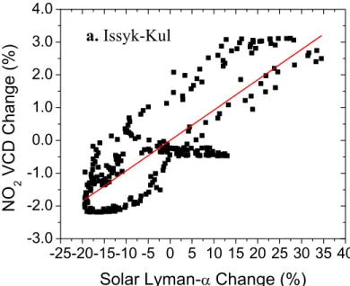
NO2 variabilities. Figure 3 shows the scatter plots of NO2 VCD changes versus the solar

Lyman-α irradiance changes over Issyk-Kul (Fig. 3a) and Kerguelen (Fig. 3b). The slope of the linear

regression represents the sensitivity of NO2 VCD to the changes in solar Lyman-α. The

correlation coefficient [R2_{] represents the goodness of the linear fit and is a measure of the}

strong positive response of NO2 to solar UV changes (near 10 % increase in NO2 VCD with

100 % increase in solar Lyman-α). The correlation of signals over station Kerguelen shows a

negative slope, suggesting a near 3 % decreasing of total NO2 with a 100 % increase in solar

Lyman-α (Fig. 3b). Note that although the extracted NO2 signal has a significant correlation with

solar UV, the correlation sometimes shows non-statistical features when the variability of NO2

does not perfectly align with the timing of solar maxima and minima.

We examined NO2 data from all 16 stations. Nine of the stations show significant positive

solar-cycle responses, with three stations showing negative or weak signals. For the remaining four

stations, we did not find any clear correlation between NO2 and Lyman-α. The analysis results

are summarized in Table 1.

5. Discussions on Analysis Results

EEMD is able to decompose a raw time series into various quasi-periodic signals, but the

decompositions may be affected by strong sporadic events. For NO2, one of the most significant

interferences comes from major volcano eruptions that inject large amounts of aerosols into the

stratosphere and cause reduction in NO2 levels. The Ultra Plinian of Mount Pinatubo eruption on

15 June 1991 produced the second-largest terrestrial eruption of the 20th century, resulting a

remarkable reduction in stratospheric NO2. The recovery of NO2 levels after the major eruption

could take a few years. Earlier studies used all available data at the time, with the Pinatubo years

in the middle of the time series (e.g. Gruzdev, 2009, 2014). While previous analysis was very

carefully carried out to simulate the corresponding aerosol impacts by using aerosol optical depth

may not be completely ruled out. Shorter time series outside the multi-year window of Pinatubo

effect could also lead to larger uncertainties in the resulting solar-cycle signals in NO2.

Therefore, to minimize the interference of Pinatubo eruption, our EEMD analysis only includes

data starting from 1996, assuming that NO2 levels had fully recovered by 1996. The time series

from 1996 to the present covers the entire Solar Cycles 23 and 24.

The results of our analysis are summarized into latitudinal-dependence patterns in Fig. 4 and

compared to those of Gruzdev (2014). Note that our results are the NO2 VCD sensitivity to

100 % Lyman-α change (left axis), while the earlier study (right axis) showed the estimated

average NO2 VCD changes between solar minimum and solar maximum for the investigated

time period (the Lyman-α change varies from one cycle to another). In the earlier study, the

extracted NO2 solar-cycle signal had no clear latitudinal dependence. Stations located at similar

latitudes often showed completely different results, with both positive and negative NO2

changes. The scatter range of the signal magnitude was wide in both hemispheres. In the present

study, the sign and magnitude of NO2 solar-cycle signal do not seem to have a clear latitudinal

dependence either. However, most of the stations with strong positive NO2 responses to solar UV

are located in the Northern Hemisphere, while the Southern Hemisphere stations show either

weak or negative NO2 solar-cycle signals. Note that some stations are located at high latitudes

where the complex NOx enhancement due to EPP in the mesosphere and the downward transport

into the stratosphere (e.g. Langematz et al., 2005; Semeniuk et al., 2011; Jackman et al., 2012)

could contribute significantly to the extracted solar-cycle signal. While the impact due to EPP

typically lasts a few days. the more frequent and stronger EPP events duing solar maximum lead

in NO2 at high latitudes could include the impacts of EPP. Moreover, the strongest solar proton

events (SPEs) often occur during the decline phase of the solar cycle, making the impacts of

these events and the UV-induced solar-cycle signal slightly out of phase. At low latitudes, the

impacts of EPP are generally small.

In addition to latitude, the altitude of the station also contributes to the differences in NO2

solar-cycle signal. Figure 5 shows the NO2 solar-cycle signal as a function of both latitude and

altitude, based on the results summarized in Table 1. The scatters are color coded according to

the percentage change in NO2 VCD with 100 % change in solar Lyman-α. The sizes of the

scatters are proportional to the correlation coefficient [R2], which is an indicator of the statistical

significance of the corresponding NO2 signal. It is clearly shown that the two stations located at

the highest altitudes, Issyk-Kul (1650 m, red circle) and Jungfraujoch (3580 m, orange circle),

have the largest positive NO2 response to solar UV. The correlation coefficients for these stations

are also among the highest. Although NDACC stations are mostly at remote areas far from local

tropospheric pollution, we cannot completely rule out the possible contribution from

tropospheric NO2. The NO2 total VCD measured at high-altitude stations does not include the

lower part of the troposphere where pollution sources are. The variability signal is therefore

more likely to be for stratospheric NO2 only. Thus the solar-cycle signals at these high altitude

stations appear to be the strongest. For stations at much lower altitudes but at very remote

locations, for example the Kerguelen Islands (located in the Southern Indian Ocean, thousands

miles away from the nearest continent), the correlation is as strong as those from the

high-altitude stations. However, the magnitude of the solar cycle response is much smaller. The

variations that could interfere with our solar cycle analysis, but could dilute the overall solar

cycle response, which is reflected in the small solar-cycle signal with a large correlation coefficient (see the large purple scatter at 49˚S in Fig. 5). For the low-altitude stations that are

not as remote, the correlations are generally weaker (shown by the smaller size of the scatters in

Fig. 5).

6. Comparison with Models

To help understand the mechanisms that control NO2 responses to solar UV changes and to

predict the corresponding impacts on O3, we performed 1D photochemical-transport model runs

to study the vertical and spectral distribution of NO2 sensitivity to solar UV change. The

Caltech/JPL 1D model covers from the surface to 130 km, with over 100 species and over 460

chemical reactions. It is currently configured for the mid-latitude conditions at Equinox.

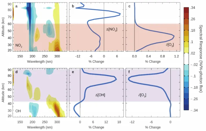
Figure 6a shows the vertically and spectrally resolved NO2 response to changes in solar UV

irradiance. The spectral NO2 response is defined as the ratio of the percentage change in NO2 to

the percentage change in solar photon flux at the top of the atmosphere (%-[NO2] / %-photon

flux). Using the percentage solar UV change as the basis, we can avoid the impact of the large

discrepancy in SSI variabilities (as mentioned in Sect. 1). By integrating the NO2 change across

the wavelength window from solar minimum to solar maximum, we calculated the overall NO2

solar-cycle variability at each altitude (Fig. 6b). The corresponding impacts on O3 purely due to

the NO2 solar-cycle changes are also calculated and shown in Fig. 6c. The largest impact on O3

is around 40 km, with the altitude range extending from about 20 km to near 60 km. Throughout

signal, which means less NO2 at solar maximum than at solar minimum, which leads to more O3

at solar maximum than minimum (Fig. 6c).

In our previous investigations on OH (Wang et al., 2013), model results suggested that the OH

solar-cycle responses have impacts on O3 above 40 km (the highlighted region is 40 – 90 km).

More OH (Fig. 7e) leads to less O3 (Fig. 7f) at solar maximum than at solar minimum.

Comparing the features in the top panels and the bottom panels in Fig.s 6, the NO2 and OH

solar-cycle effects on O3 have completely opposite directions. Their combined effects determine the

solar-cycle change in middle atmospheric O3. In the upper middle atmosphere, OH effects

dominate and more OH leads to less O3. Between 40 – 60 km where the two effects overlap, they

partially cancel out, leading to smaller O3 variabilities due to solar cycles. At the lower part of

the middle atmosphere, below 40 km, NO2 effects plays a more important role.

In order to fully understand the chemical mechanisms behind the NO2 solar-cylce response

pattern in Fig. 6a, we investigated the precursors of NO2 and the key chemical reation rates. Fig.

7 shows the vertically and spectrally resolved response of the key species and chemical reactions

to the changes in solar UV irradiance. The spectral response functions highlight individual

chemical reactions involved in the NOx solar-cycle responses, which helps isolate the dynamical

impacts in 3D models.

The stratospheric NO2 mainly comes from reaction 4, the reaction of NO (Fig. 7b) with O3 (Fig.

7e). As seen in Fig. 7a, with the increasing solar UV flux at solar maxima, NO2 shows a strong

negative response around 200 nm throughout the middle atmosphere and an extended positive

response around 300 nm thoughout the middle atmosphere, especially in the stratosphere. A

smaller positive response at 35 – 55km and a smaller negative response at 40 – 60 km are also

shown. These responses partially cancel out with each other, resulting the overall negative

vertical profile of NO2 solar-cycle signal in Fig. 6b.

The features of NO2 UV responses in Fig. 7a clearly resemble the responses of its production

rate through reaction 4 (NO + O3  NO2 + O2) in Fig. 7f. The combination of the responses in

NO (Fig. 7b) and O3 (Fig. 7d) thus explains the patterns in Fig. 7f as well as Fig. 7a. To further

understand Fig. 7b, the NO responses to UV changes, we need to analyze its source species N2O

and O(1D). When solar UV increases, O(1D) is enhenced via two photolysis reactions 2 and 3: O3

+ h  O2 + O(1D) and N2O + h  N2 + O(1D). The enhanced N2O loss through its direct

photolysis, reaction 3, leads to the strong negative N2O response around 200 nm. The decreasing

effect at lower altitudes is clearly due to the rapidly decreasing UV as light penetrating through

the stratosphere. The much weaker negative N2O response around 300 nm is most likely a result

of the enhanced N2O loss through its reaction with increasing O(1D). This hypothesis is

confirmed by the strong positive O(1D) response (Fig. 7e) and the negative O3 response (Fig. 7d)

at the same wavelengths with very similar patterns. The other positive O(1D) response at shorter

wavelengths (below 240 nm) and above 35 km is due to the enhanced photolysis of O2 at the

corresponding wavelengths. The negative O(1_{D) response at below 35 km is a typical result of}

the atmospheric shielding effect – The enhanced O3 during solar maxima at these wavelengths

part of the stratosphere. This shielding effect results in less short-wavelength UV available at

below 35 km for O2 photolysis and O(1D) production at the corresponding wavelengths. These

combined effects of N2O and O(1D) result in the NO responses to solar UV changes. NO quickly

reacts with O3 in the NOx cycle; updating the equilibrium state with NO2 and Thus the reaction

between NO and O3 determines the changes in NO2. The spectral response of NO2 (Fig. 7a) is

therefore very similar to those of the direct NO2 production rate through NO + O3  NO2 + O2

(Fig. 7f); the latter is close to a direct sum of the spectral responses in NO and O3 (Fig.s 7b and

7d), as expected in the photochemical equilibrium. This analysis decomposes the chemical

machnisms governing the NOx solar-cycle responses, which is very important for understanding

the NO2 variabilities in more complex 3D models and to identify the impacts from dynamics.

While the 1D model predicts a negative NO2 solar-cycle signal throughout the highlighted

altitude region (20 – 60 km) where NO2 plays an important role controlling O3, most NDACC

stations show positive NO2 solar-cycle signals in the observed NO2 VCD. In the previous study

by Gruzdev (2014), the comparison between NDACC observations and 2D model results showed

similar discrepancies.

Due to the strong diurnal variability, NO2 as well as the solar zenith angle (SZA) change rapidly

during sunrise and sunset when NDACC NO2 VCD measurements are carried out. The changes

in the observed NO2 solar-cycle signal during the measurement time window have to be

quantified. We did sensitivity studies with the 1D model to investigate the sensitivity of NO2

solar-cycle signals to the time of day. Figure 8 shows the calculated NO2 variability between

and sunset. The resulting vertical profiles are somewhat different in the magnitude. However, the

negative sign remains for all cases. Therefore, the fact that measurements might not be always

carried out at exactly the same SZA could possibly introduce additional uncertainties to the

magnitude of the extracted solar-cycle signal, but will not change the sign of it.

Besides geo-locations (altitude and latitude) and the measurement time, other factors that could

also contribute to the observed signals in Fig. 5 include the distance from major pollution sources

and long-range atmospheric transport. The impacts due to these factors may be examined using

global 3D chemistry-transport models.

As a preliminary investigation, Fig. 9 shows the zonally averaged NO2 solar-cycle signals

extracted from the CCMI WACCM-SD model run from 1979 to 2014. In order to investigate the

contribution of NO2 variability in each vertical grid to the total VCD NO2 variability, we present

the model calculated NO2 solar-cycle signal as the corresponding NO2 VCD changes (%) per

100% change in Lyman-α changes at each vertical interval of 1 km. The patterns in different

seasons are shown in the four panels: 9a (December – February), 9b (March – May), 9c (June –

August), and 9d (September – November). There is a seasonal difference on top of the vertical

and latitudinal patterns. At mid-latitudes, the NO2 solar-cycle signal is generally negative or very

small (in agreement with the 1D model results), except for the thin layer at the bottom of the

middle atmosphere (40 – 100 hPa) where NO2 solar-cycle signal has a significant positive value.

This positive NO2 solar-cycle signal is especially strong at the tropical region and is generally

stronger in the northern hemisphere than in the southern hemisphere, which leads to an overall

This is consistent with the mostly positive solar-cycle signals in NO2 VCD data from NDACC

stations in the northern hemisphere and the weak or negative signals in NO2 VCD from stations

in the southern hemisphere. The seasonal difference at these latitudes is not very strong. This

layer of strong positive NO2 solar-cycle signal was not predicted in our 1D model or the 2D

model used by Gruzdev (2014). Thus, the positive solar response in the NO2 column observed

over the NDACC network is likely a result of the general circulation. The simpler 1D or 2D

models are not adequate to reveal these complex features, resulting in the apparent discrepancies

in NO2 solar-cycle variability between NDACC observations and 2D models as reported by

Gruzdev (2014).

At high latitudes where the dynamics of polar vortex and the EPP effects play a crucial role (e.g.

Langematz et al., 2005; Semeniuk et al., 2011), the model results show totally different patterns.

The high-latitude NO2 variability is far more complex than at mid- to low-latitudes. The dramatic

seasonal differences and the deep vertical extension of the high-latitude NO2 solar-cycle

variability suggest significant impacts of NO2 intrusions from the mesosphere, especially during

the polar winter (see the North Pole in Fig. 9a and the South Pole in Fig. 9c). Further

investigations with models specialized in polar chemistry and transport (including polar vortex

dynamics and accurate prescription of the solar proton events and energetic electron

precipitation, etc.) are needed to fully understand the high-latitude NO2 variability. At mid- to

low-latitudes where the contribution of mesospheric NO2 variability is much smaller, the

observed total column NO2 variability comes mostly from the stratosphere.

To see how the complex responses in the 3D model may impact the ground-based observations,

we integrate the WACCM-SD NO2 concentration from 250 hPa to 0.7 hPa (focus on the

change over the 11-year solar cycle (shown in Fig. 10 as the blue-solid line). The annual average

corresponds to a robust solar response that is expected if we had a globally dense surface

network. The resultant NO2 solar response exhibits a double-well structure: there is a positive

maximum of about 8 % near the Equator due to the thin layer of positive NO2 changes in the

lower stratosphere (shown in Fig. 9), and two negative minima of about –3 % in northern and

southern subtropics due to photochemistry. Beyond 60° latitude, the polar dynamics is dominant

and the solar response is strongly positive. To further isolate the photochemical effect at low

latitudes, we calculate the solar response in the upper stratospheric region from 10 hPa to 0.7 hPa

(Fig. 10, pink-dashed line), which is predominantly negative of about –3% below 60° latitude.

The tropical maximum is solely due to the lower stratospheric response, as is shown by the

orange-dashed line in Fig. 10. For comparison, the upper-stratospheric response (pink-dashed

line) agrees with the 2D model simulation used by Gruzdev (2009) (Fig. 10, green-thick line).

We also integrate the NO2 column in our 1D model from 12 km to 50 km. The 1D model result

shows that, without any meridional circulation, the tropical solar response may be slightly more

negative, which is –3.4 % in the diurnal average (Fig. 10, black triangle).

Lastly, we compare the simulated stratospheric NO2 solar-cycle response with the NDACC

observations in Fig. 4. In contrast to Gruzdev’s (2014) linear regression, our EMD-extracted

more positive solar-cycle responses in the northern hemisphere agree better with the WACCM

simulation, thus revealing the influence of EPP-induced NO2 in the northern stratosphere.

However, the EMD-extracted solar-cycle responses from 4 stations in the southern hemisphere

are much lower than the WACCM-SD simulation, suggesting that the observed EPP-induced

the zonal averaging of the WACCM-SD simulation, we have performed another calculation

using only the time series at model grid points closest to the four stations and verified that the

simulated NO2 solar-cycle responses at those grid points remain the same as in the zonal

averages. Unfortunately, there is not enough NDACC measurements of NO2 column to confirm

the positive response in the tropical region.

The WACCM-SD result discussed above implies that dynamics in the tropical lower stratosphere

and the polar stratosphere is the dominant contributing factor of the positive sign of the

simulated NO2 solar-cycle responses. Note that the ground-based measurements of total column

NO2 also consists of a significant fraction (20 % or less, depending on the altitude of the

station) from the tropospheric that could be affected by a number of factors such as urban

sources (less possible due to the remote location of many of the stations) and the tropospheric

circulation. The local NO2 solar responses over the NDACC stations likely contributed to the

more scattered variability in Fig. 4 than the smooth responses predicted by photochemistry and

WACCM-SD. The double-well structure as simulated in WACCM-SD may serve as a critical

test of dynamics impacts that are missing in the 1D or 2D models. Continuous network

measurements and long-term satellite measurements of NO2 are crucial for further improving our

ability to understand the coupled effects of atmospheric dynamics and chemistry.

7. Conclusions

The response of NO2 to solar UV irradiance changes during the most recent two solar 11-year

cycles was quantified using long-term observations from NDACC stations and compared with

We use EEMD approach to separate the NO2 solar-cycle signal from the variabilities of other

time scales as well as the longer-term trend. A positive correlation between the extracted

solar-cycle mode of NO2 with solar Lyman-α is found for data over nine stations, while a negative

correlation is reported for three stations. The stations with strong or moderate positive NO2

solar-cycle responses are all located in the Northern Hemisphere, leaving the Southern Hemisphere

stations with weak or negative NO2 responses. Further correlations with altitude show that the

stations with the highest altitudes and the minimal interference of tropospheric variabilities have

the strongest positive NO2 responses to solar cycles. At high latitudes where EPP could play a

significant role in the stratospheric NO2 variabilities, the extracted solar cycle signals could

include responses due to both solar UV and the EPP.

At low latitude where the EPP-induced NO2 signal is negligible, we use a 1-D photochemical

model to study the direct UV-induced NO2 solar-cycle response definitively. The detailed

analysis of the spectral responses of NOx and their precursor spices explains the spectral regions

and the altitude ranges where NOx show positive or negative responses to the soalr UV changes.

Our results suggest that the variability in NO2 and the corresponding NOx–O3 chemistry plays an

important role for O3 at the altitude range of about 20 km to near 60 km, with 40 km being the

center of the peak effect. Since OH variability and the HOx–O3 chemistry is believed to control

O3 variability at the upper middle atmosphere above 40 km, our results suggests that, at the 40 –

60 km region, the combined effects of NOx and HOx likely determine the variability in the O3

catalytic loss. Above 60 km, the chemical loss of O3 is likely dominated by HOx chemistry.

In contrast to the positive NO2 solar-cycle signal over most of the NDACC stations, the signal

predicted by the 1D model is negative throughout the altitude region where NOx is important for

O3, which agrees with the 2D modeling work by Gruzdev (2014), who showed that such a

negative response holds almost globally except the deep polar regions. While the stations are

located at remote areas or far from pollution sources, interferences from tropospheric NO2 cannot

be completely ruled out. The fact that the NDACC stations reveal scattered NO2 responses at

similar latitudes also suggests that dynamics may play an important role. Thus, we also

investigate the NO2 solar-cycle signal simulated by WACCM-SD. We found hints of a complex

seasonal difference in addition to the vertical and latitudinal patterns. The vertical profile of NO2

solar-cycle response is more complex than in the 1D model. In particular, the WACCM-SD

results reveal a significant positive NO2 response at the bottom of the stratosphere at mid- and

low-latitudes. This feature, together with the negative UV-induced NO2 response (as shown by

the 1D model results) and the EPP-induced response at high latitudes, creates a unique

double-well structure as a result of the coupled effects of atmospheric dynamics and chemistry.

Continuous network measurements and long-term satellite measurements of NO2 are required to

verify the simulated double-well structure.

This work provides new evidence of NO2 response to solar cycles to help resolve the

long-standing puzzles in the field.

Acknowledgments

We acknowledge the support from the NASA Living with a Star (LWS) program (“Solar Forcing

NO2 VCD data used in this publication were obtained from the Network for the Detection of

Atmospheric Composition Change (NDACC) and are publicly available (www.ndaccdemo.org/).

We thank Valery P. Sinyakov at the Kyrgyz National University, Kyrgyz Republic, for sharing

data over Issyk-Kul, Michel Van Roozendael and François Hendrick at the Belgian Institute for

Space Aeronomy (BIRA-IASB) for sharing data over the Jungfraujoch and Harestua, Udo Frieß

at the Institute of Environmental Physics, University of Heidelberg, for sharing data over

Neumayer (Frieß, et al., 2005), Geraint Vaughan at University of Manchester for sharing data

over Aberystwyth, Paul V. Johnston (Emeritus) at the National Institute of Water & Atmospheric

Research Ltd (NIWA), New Zealand, for sharing data over Kiruna. The solar Lyman-alpha

composite used in this work includes measurements from multiple instruments and models. It

was provided by Martin Snow from the LASP Interactive Solar Irradiance Datacenter

(lasp.colorado.edu/lisird/ ).

Disclosure of Potential Conflicts of Interest

The authors declare that they have no conflicts of interest.

References

Allen, M., Lunine, J.I., Yung, Y.L.: 1984, The vertical distribution of ozone in the mesosphere

and lower thermosphere. J. Geophys. Res. 89, 4841, doi:10.1029/JD089iD03p04841.

Allen, M., Yung, Y.L., Waters, J.W.: 1981, Vertical transport and photochemistry in the

terrestrial mesosphere and lower thermosphere (50-120km). J. Geophys. Res. 86, 3617,

Ball, W.T., Mortlock, D.J., Egerton, J.S., Haigh, J.D.: 2014, Assessing the relationship between

spectral solar irradiance and stratospheric ozone using Bayesian inference. J. Space Weather

Space Clim. 4, A25, doi:10.1051/swsc/2014023.

Bauer, R., Rozanov, A., McLinden, C.A., Gordley, L.L., Lotz, W., Russell III, J.M., Walker,

K.A., et al.: 2012, Validation of SCIAMACHY limb NO2 profiles using solar occulation

measurements. Atmos. Meas. Tech., 5, 1059-1084, doi:10.5194/amt-5-1059-2012.

Beig, G., Fadnavis, S., Schmidt, H., Brasseur, G.P.: 2012, Inter-comparison of 11-year solar

cycle response in mesospheric ozone and temperature obtained by HALOE satellite data and

HAMMONIA model. J. Geophys. Sci. 117, D00P10, doi:10.1029/2011JD015697.

Boersma, K. F., Eskes, H. J., Dirksen, R. J., van der A, R. J., Veefkind, J. P., Stammes, P.,

Huijnen, V., et al.: 2011, An improved retrieval of tropospheric NO2 columns from the Ozone

Monitoring Instrument. Atmos. Meas. Tech., 4, 1905-1928, doi:10.5194/amt-4-1905-2011.

Brasseur, G.P. and Solomon. S.: 2005, Aeronomy of the middle atmosphere: Chemistry and

physics of the stratosphere and mesosphere. Third edition, Springer, Dordrecht, the Netherlands.

Dirksen, R.J., Boersma, K.F., Eskes, H.J., Ionov, D.V., Bucsela, E.J., Levelt, P.F., Kelder, H.M.:

2011, Evaluation of stratospheric NO2 retrieved from the Ozone Monitoring Instrument:

Intercomparison, diurnal cycle, and trending. J. Geophys. Res., 116, D08305,

doi:10.1029/2010JD014943.

Ermolli, I., Matthes, K., Dudok de Wit, T., Krivova, N.A., Tourpali, K., Weber, M., et al.: 2013,

Recent variability of the solar spectral irradiance and its impact on climate modeling. Atmos.

Frieß, U., Kreher, K., Johnston, P., Platt, U.: 2005, Ground-based DOAS measurements of

stratospheric trace gases at two Antarctic stations during the 2002 ozone hole period, J. Atmos.

Sci. 62, 765.

Garcia, R.R., López-Puertas, M., Funke, B., Marsh, D.R., Kinnison, D.E., Smith, A.K., and

González-Galindo F.: 2014, On the distribution of CO2 and CO in the mesosphere and lower

thermosphere, J. Geophys. Res. Atmos. 119, 5700–5718, doi:10.1002/2013JD021208.

Gruzdev, A.N.: 2008, Latitudinal dependence of variations in stratospheric NO2 content. Atmos.

Ocean. Phys. 44, 319, doi:10.1134/S0001433808030079.

Gruzdev, A.N.: 2009, Latitudinal structure of variations and trends in stratospheric NO2. Int. J.

Rem. Sens. 30, 4227, doi:10.1080/01431160902822815.

Gruzdev, A.N.: 2014, Estimate of the effects of Pinatubo eruption in stratospheric O3 and NO2

contents taking into account the variations in the solar activity. Atmos. Oceanic Opt. 27, 403,

doi:10.1134/S102485601405008X.

Haigh, J.D., Winning, A.R., Toumi, R., Harder, J.W.: 2010, An influence of solar spectral

variations on radiative forcing of climate. Nature 467, 696, doi:10.1038/nature09426.

Hendrick, F., Mahieu, E., Bodeker, G.E., Boersma, K.F., Chipperfield, M.P., De Maziere, M.,

et al.: 2012, Analysis of stratospheric NO2 trends2 trends above Jungfraujoch using

ground-based UV-visible, FTIR, and satellite nadir observations. Atmos. Chem. Phys. 12, 8851–8864.,

doi:10.5194/acpd-12-8851-2012.

Hood, L.L., Soukharev, B.E.: 2006, Solar induced variations of odd nitrogen: Multiple regression

Huang, N.E., Shen, Z., Long, S.R., Wu, M.L.C., Shih, H.H., Zheng, Q.N., et al.: 1998, The

empirical mode decomposition and the Hilbert spectrum for nonlinear and non-stationary time

series analysis. Proc. R. Soc. Lond. A 454, 903, doi:10.1098/rspa.1998.0193.

Jacob, D. J.: 1999, Introduction to Atmospheric Chemistry,. Princeton University Press.

Johnston, P. V., McKenzie, R. L.: 1989, NO2 observations at 45°S during the decreasing phase

of solar cycle 21, from 1980 to 1987. J. Geophys. Res. 94, 3473,

doi:10.1029/JD094iD03p03473.

Kobayashi-Kirschvink, K.J., Li, K. F., Shia, R.-L. Yung, Y.L.: 2012, Fundamental modes of

atmospheric CFC-11 from empirical mode decomposition. Adv. Adaptive Data Anal. 4,

1250024, doi:10.1142/S1793536912500240.

Langematz, U., Grenfell, J.L., Matthes, K., Mieth, P., Kunze, M., Steil, B., and Bruhl, C.: 2005,

Chemical effects in 11-year solar cycle simulations with the Freie Universität Berlin Climate

Middle Atmosphere Model with online chemistry (FUB-CMAM-CHEM). Geophys. Res. Lett.,

32, L13803, doi: 10.1029/2005GL022686.

Li, K.-F., Zhang, Q., Tung, K.-K., Yung, Y.L.: 2016, Resolving a long-standing

model-observation discrepancy on ozone solar cycle response. Earth and Space Sci. 431.

doi:10.1002/2016EA000199.

Liley, J.B., Johnson, P.V., McKenzie, R.L., Thomas, A.J., Boyd, I.S.: 2000, Stratospheric NO2

variations from a long time series at Lauder, New Zealand. J. Geophys. Res. 105, 11633–11640,

doi:10.1029/1999JD901157.

Machol, J., Snow, M., Woodraska, D., Woods, T., Viereck, R., Coddington, O.: 2019, An

Maeda, S., Fuller-Rowell, T.J., and Evans, D.S.: 1989, Zonally averaged dynamical and

compositional response of the thermosphere to auroral activity during September 18–24, 1984, J.

Geophys. Res., 94(A12), 16869–16883, doi:10.1029/JA094iA12p16869.

Marsh, D., Mills, M.J., Kinnison, D.E., Garcia, R.R., Lamarque, J.-F., Calvo, N.: 2013, Climate

change from 1850–2005 simulated in CESM1 (WACCM). J. Climate 26, 7372–7391,

doi:10.1175/JCLI-DD-12-00558.1.

Merkel, A.W., Harder, J.W., Marsh, D.R., Smith, A.K., Fontenla, J.M., Woods, T.N.: 2011, The

impact of solar spectral irradiance variability on middle atmospheric ozone. Geophys. Res. Lett.

38, L13802, doi:10.1029/2011GL047561.

Mills, F. P., Cageao, R.P., Sander, S.P., Allen, M., Yung, Y.L., Remsberg, E.E., et al.: 2003, OH

Column Abundance Over Table Mountain Facility, California: Intra-annual Variations and

Comparisons to Model Predictions for 1997–2001. J. Geophys. Res. Atmos, 108, 4785,

doi:10.1029/2003JD003481.

Morgenstern, O., Hegglin, M.I., Rozanov, E., O'Connor, F.M., Abraham, N.L., Akiyoshi, H., et

al.: 2017, Review of the global models used within phase 1 of the Chemistry–Climate Model

Initiative (CCMI), Geosci. Model Dev. 10, 639, doi:10.5194/gmd-10-639-2017.

Newman, S., Xu, X., Gurney, K.R., Hsu, Y.K., Li, K.L., Jiang, X., et. al.: 2016, Toward

consistency between trends in bottom-up CO2 emissions and top-down atmospheric

measurements in the Los Angeles megacity. Atmos. Chem. Phys. 16, 3843, doi:

10.5194/acp-16-3843-2016.

Peck, E.D., Randall, C.E., Harvey, V.L. and Marsh, D.R.: 2015, Simulated solar cycle effects on

doi:10.1002/2014MS000387.

Remsberg, E.E.: 2008, On the response of Halogen Occultation Experiment (HALOE)

stratospheric ozone and temperature to the 11-year solar cycle forcing. J. Geophys. Res. 113,

D22304., doi:10.1029/2008JD010189.

Remsberg, E.E.: 2008, On the response of Halogen Occultation Experiment (HALOE)

stratospheric ozone and temperature to the 11-year solar cycle forcing. J. Geophys. Res. 113,

D22304., doi:10.1029/2008JD010189.

Remsberg, E.E.: 2013, Decadal-scale responses in middle and upper stratospheric ozone from

SAGE II version 7 data. Atmos. Chem. Phys. Discuss. 13, 20239,

doi:10.5194/acpd-13-20239-2013.

Rusch, D.W., Gerard, J.-C., Solomon, S., Crutzen, P.J., and Reid, G.C.: 1981, The effect of

particle precipitation events on the neutral and ion chemistry of the middle atmosphere – I. odd

nitrogen. Planet Space Sci. 29(7), 767 – 774.

Semeniuk, K., Fomichev, V.I., McConnell, J.C., Fu, C., Melo, S.M.L, and Usoskin, I.G.: 2011,

Middle atmosphere response to the solar cycle in irradiance and ionizing particle precipitation.

Atmos. Chem. Phys., 11, 5045-5077, doi:10.5194/acp-11-5045-2011.

Shi, Y., Li, K.-F., Yung, Y.L., Aumann, H.H., Shi, Z., Hou, T.Y.: 2013, Principal modes of

variability in the tropics from 9-Year AMSU data. Climate Dyn. 41, 1385,

doi:10.1007/s00382-013-1696-x.

Solanki, S.K., Krivova, N.A., Haigh, J.D.: 2013, Solar irradiance variability and climate. Annual

Ann. Rev. of Astron. Astrophys. 51, 311. doi:10.1146/annurev-astro-082812-141007.

Geophys. 37, 275. doi:10.1029/1999RG900008.

Swartz, W.H., Stolarski, R.S., Oman, L.D., Fleming, E.L., Jackman, C.H.: 2012, Middle

atmosphere response to different descriptions of the 11-yr solar cycle in spectral irradiance in a

chemistry-climate model. Atmos. Chem. Phys., 12, 5937, doi:10.5194/acp-12-5937-2012.

Tapping, K.F.: 2013, The 10.7 cm solar radio flux (F10.7), Space Weather 11, 394,

doi:10.1002/swe.20064.

Wang, S., Li, K-F., Pongetti, T.J., Sander, S.P., Yung, Y.L., Liang, M.-C., et al.: 2013,

Atmospheric OH response to the most recent 11-year solar cycle. Proc. Natl. Acad. Sci. 110,

2023–2028, doi: 10.1073/pnas.1117790110

Wang, S., Zhang, Q., Millan, L., Li, K.-F., Yung, Y.L., Sander, S.P., et al.: 2015, First evidence

of middle atmospheric HO2 response to 27-day solar cycles from satellite observations. Geophys.

Res. Lett. 42, 10004, doi:10.1002/2015GL065237.

Woods, T.N., Tobiska, W.K., Rottman, G.J., Worden, J.R.: 2000, Improved solar Lyman α

irradiance modeling from 1947 through 1999 based on UARS observations. J. Geophys. Res.

Space Phys. 105, A12, 27195. doi: 10.1029/2000JA000051.

Wu, Z., Huang, N.E.: 2009, Ensemble empirical mode decomposition: A noise-assisted data

analysis method. Adv. Adaptative Data Analysis 1, 1, doi:10.1142/S1793536909000047.

Yung, Y.L., DeMore, W.D.: 1999, Photochemistry of Planetary Atmospheres, Oxford University

Press, Oxford.

Figure 1. EEMD decomposition results for station Issyk-Kul. Left panels are timeseries of NO2

signals [1015 cm-2], with the raw data on the top and decomposed signals below. Right columns

show the corresponding power spectra. For the raw data, the power spectrum is obtained using

marginal Hilbert spectrum (MHS). The residual is the longer-term trend on top of the baseline

Figure 2. EEMD decomposition results for station Kerguelen. Left panels are signals, with the

raw data [1013 cm-2] on the top and decomposed signals below. Right columns show the

corresponding power spectra. The residual is the longer-term trend on top of the baseline value.

Figure 3. Linear correlation of the extracted NO2 solar-cycle signal (from Figs. 1 and 2) and

Figure 4. Latitudinal pattern of the NO2 sensitivity to solar Lyman-α change. The analysis results

from this study are shown in orange. The numbers stand for percentage change in NO2 VCD

with 100% change in solar Lyman-α. The NO2 VCD solar-cycle variability [%] from Gruzdev

Figure 5. The altitude and latitude dependence of the NO2 sensitivity to solar Lyman-α change.

The scatters are color-coded according to the percentage change in NO2 VCD with 100 %

change in solar Lyman-α. The sizes of the scatters are proportional to the correlation coefficient

Figure 6. Vertical profile of NO2 solar-cycle signal in comparison with OH solar-cycle signal

and their implications for O3 from the 1D model. (a) The vertically and spectrally resolved NO2

response (% change in NO2) to changes in solar UV irradiance (% change in the photon flux). (b)

Vertical profiles of NO2 solar-cycle signal from the model. (c) The corresponding O3 variability

solely due to the changes in NO2 in Panel b. The highlighted altitude region (≈20 – 60 km)

shows where NO2 solar-cycle changes have significant impacts on O3. Panels d, e, and f are the

same as Panels a, b, and c except that they are for OH instead of NO2. The highlighted altitude

region (≈40 – 90 km) shows where OH solar-cycle changes have significant impacts on O3. See

Figure 7. The vertically and spectrally resolved response of chemical species and key chemical

Figure 8. Changes in NO2 number density [107 molecules cm-3] between solar maximum and

Figure 9. CCMI WACCM SD model run from 1979 to 2014. The NO2 solar-cycle response in

each of the four seasons is shown as the corresponding changes in NO2 VCD (%) per 100%

change in solar Lyman-α changes at each vertical interval of 1 km. (a) December – February, (b)

Figure 10. The 11-year solar-cycle response of vertically integrated NO2 from the WACCM

Specified Dynamics (WACCM-SD) model run. The blue, orange, and pink lines represent results

from different vertical ranges of the NO2 column integration. The results of the 2D model used

by Gruzdev (2009) are shown by the green-thick line. The corresponding result of the 1D model

in this work (24-hour diurnal average) is marked by the black triangle. The unit is %-NO2 VCD

Station Latitude [°] Longitude [°] Altitude [m ASL] NO2 solar-cycle signal [% change/100% change in Lyman-α] Error R2 Neumayer -70.62 8.37E 42 -0.27 0.02 0.58 Dumont -66.67 140.0E 20 1.6 0.2 0.14 Kerguelen -49.3 70.3E 10 -2.7 0.1 0.61 Lauder -45.04 169.68W 370 2.1 0.2 0.38 Issk-Kul 42.6 77.0E 1650 9.3 0.4 0.69 Jungfraujoch 46.55 7.98E 3580 7.4 0.6 0.45 Aberystwyth 52.4 4.1W 50 5.3 0.4 0.42 Harestua 60.2 10.8E 596 2.9 0.4 0.18 Zhigansk 66.8 123.4E 50 8.3 1 0.26 Sodankyla 67.37 26.65E 179 4.6 0.6 0.18 Kiruna 67.84 20.41E 419 -1.1 0.1 0.39 Scorebysund 70.48 21.97W 68 5.9 0.4 0.43

Table 1. Summary of the 12 stations with significant NO2 solar-cycle signal.

The % response in NO2 VCD is determined by the slope in the linear correlation between NO2

changes and Lyman-α changes (as shown in Fig. 3). The error bar is determined by the

uncertainty of the linear regression. The correlation coefficient [R2_{] represents the goodness of}