Inter-hemispheric linkages in climate change: paleo-perspectives for future climate change

HAL Id: hal-00298056

https://hal.archives-ouvertes.fr/hal-00298056

Submitted on 26 Oct 2006

HAL is a multi-disciplinary open access

archive for the deposit and dissemination of

sci-entific research documents, whether they are

pub-lished or not. The documents may come from

teaching and research institutions in France or

abroad, or from public or private research centers.

L’archive ouverte pluridisciplinaire HAL, est

destinée au dépôt et à la diffusion de documents

scientifiques de niveau recherche, publiés ou non,

émanant des établissements d’enseignement et de

recherche français ou étrangers, des laboratoires

publics ou privés.

Inter-hemispheric linkages in climate change:

paleo-perspectives for future climate change

J. Shulmeister, D. T. Rodbell, M. K. Gagan, G. O. Seltzer

To cite this version:

J. Shulmeister, D. T. Rodbell, M. K. Gagan, G. O. Seltzer. Inter-hemispheric linkages in climate

change: paleo-perspectives for future climate change. Climate of the Past, European Geosciences

Union (EGU), 2006, 2 (2), pp.167-185. �hal-00298056�

www.clim-past.net/2/167/2006/

© Author(s) 2006. This work is licensed under a Creative Commons License.

Climate

of the Past

Inter-hemispheric linkages in climate change: paleo-perspectives for

future climate change

J. Shulmeister1, D. T. Rodbell2, M. K. Gagan3, and G. O. Seltzer4†

1_{Department of Geological Sciences, University of Canterbury, Private Bag 4800, Christchurch, New Zealand} 2_{Department of Geology, Union College, Schenectady, NY 12308, USA}

3_{Research School of Earth Sciences, The Australian National University, Canberra 2000, ACT, Australia} 4_{Department of Earth Sciences, Heroy Geology Lab, University of Syracuse, Syracuse NY 13244, USA} †_deceased

Received: 20 December 2005 – Published in Clim. Past Discuss.: 22 February 2006 Revised: 31 August 2006 – Accepted: 16 October 2006 – Published: 26 October 2006

Abstract. The Pole-Equator-Pole (PEP) projects of the PANASH (Paleoclimates of the Northern and Southern Hemisphere) programme have significantly advanced our un-derstanding of past climate change on a global basis and helped to integrate paleo-science across regions and research disciplines. PANASH science allows us to constrain predic-tions for future climate change and to contribute to the man-agement of consequent environmental changes. We identify three broad areas where PEP science makes key contribu-tions.

1. The pattern of global changes. Knowing the exact timing of glacial advances (synchronous or otherwise) dur-ing the last glaciation is critical to understanddur-ing inter-hemispheric links in climate. Work in PEPI demonstrated that the tropical Andes in South America were deglaciated earlier than the Northern Hemisphere (NH) and that an ex-tended warming began there ca. 21 000 cal years BP. The general pattern is consistent with Antarctica and has now been replicated from studies in Southern Hemisphere (SH) regions of the PEPII transect. That significant deglaciation of SH alpine systems and Antarctica led deglaciation of NH ice sheets may reflect either i) faster response times in alpine systems and Antarctica, ii) regional moisture patterns that in-fluenced glacier mass balance, or iii) a SH temperature forc-ing that led changes in the NH. This highlights the limitations of current understanding and the need for further fundamen-tal paleoclimate research.

2. Changes in modes of operation of oscillatory climate systems. Work across all the PEP transects has led to the recognition that the El Ni˜no Southern Oscillation (ENSO) phenomenon has changed markedly through time. It now ap-pears that ENSO operated during the last glacial termination Correspondence to: J. Shulmeister

(james.shulmeister@canterbury.ac.nz)

and during the early Holocene, but that precipitation tele-connections even within the Pacific Basin were turned down, or off. In the modern ENSO phenomenon both inter-annual and seven year periodicities are present, with the inter-annual signal dominant. Paleo-data demonstrate that the relative im-portance of the two periodicities changes through time, with longer periodicities dominant in the early Holocene.

3. The recognition of climate modulation of oscillatory systems by climate events. We examine the relationship of ENSO to a SH climate event, the Antarctic cold reversal (ACR), in the New Zealand region. We demonstrate that the onset of the ACR was associated with the apparent switching on of an ENSO signal in New Zealand. We infer that this re-lated to enhanced zonal SW winds with the amplification of the pressure fields allowing an existing but weak ENSO sig-nal to manifest itself. Teleconnections of this nature would be difficult to predict for future abrupt change as boundary conditions cannot readily be specified. Paleo-data are critical to predicting the teleconnections of future changes.

1 Introduction

1.1 Background to the Pole-Equator-Pole projects of PANASH

The aim of all PANASH science is to understand the modes of climate and environmental variability. This work is prob-lem/project focused. The ENSO climate system, for exam-ple, has been a particular focus for research. These research problems are tackled through multi-proxy climate and envi-ronmental reconstructions and paleo-climate modeling.

Within PANASH, the largest projects have been the three PEP transects. PEP I covers the Americas, PEPII covers

168 J. Shulmeister et al.: PEP overview the East Asia to Australasia region, and PEPIII extends from

Northern Europe to Southern Africa. Under the auspices of the PEPs hundreds of scientists have been involved in dozens of projects. The PEPs have played a major role in bringing together disparate regions and research disciplines into co-hesive science programmes and numerous, substantive out-puts have been achieved (e.g. Markgraf, 2001; Battarbee et al., 2004; Dodson et al., 2004). Given the scale of the PEP projects, it is not feasible to attempt to summarise the whole of the science programme in a single paper. Instead this paper identifies three general areas of research where PEP projects have significantly contributed to the understanding of past and present climate systems. In order to further focus the paper we have chosen to review progress in one region, the South Pacific Basin, using a case study approach.

We highlight how the understanding derived from “paleo” work can assist in the understanding of future change. We fo-cus on the need to work on high-resolution records that will allow paleoclimate science to interface with climate mod-elling and management but we also emphasise the need for on-going fundamental research into past environments and climates. Despite many decades of paleoenvironmental re-search we do not have adequate understanding of the patterns of change over huge swathes of the globe’s surface, notably Africa, the SH in general and much of the world’s oceans.

The three topics we have chosen to highlight are: 1) Pat-terns of global change, 2) Changes in the modes of oscil-latory climate systems, and 3) Climatic teleconnections of climate events. The latter two topics deal with the unique power of ‘paleo’ science to deal with longer-term changes and extreme events. The first topic, however, highlights a cautionary note about the limits of our knowledge.

2 Contribution 1: The pattern of global changes: Case study – The Last Glacial Maximum (LGM) and the timing of deglaciation in the Southern tropics and mid-latitudes

One of the longest standing debates in global climate change has been on the mechanism of climate signal transfer from the region of climate forcing to the rest of the globe. The largest climate changes of the recent geological past are the ice ages. On a glacial-interglacial timescale, the timing of glacial advances in the mid-latitude SH appears to be broadly synchronous with those of the main northern ice advances (e.g. Nelson et al., 1985). This is unexpected, as SH con-ditions based on orbital (Milankovitch) forcing of solar in-solation, should be out of phase with the Northern Hemi-sphere (Mercer, 1984; Berger, 1992). The apparent syn-chrony requires rapid transfer of cooling from the North-ern Hemisphere (NH). The main candidates for this forcing are changes in greenhouse gas concentration in the atmo-sphere (e.g. Petit et al., 1999; Inderm¨uhle et al., 2000) and/or

changes in heat transport through ocean (thermohaline) cir-culation (e.g. Broecker, 2000; Stocker, 2000).

The focus for much of this work has centred on the ter-mination of the last ice-age. The primary reason for this is that the warming associated with this termination is of simi-lar or even simi-larger magnitude than the human-induced climate modification expected under future greenhouse-gas scenar-ios (Watson et al., 2001) although the rate of change was much slower. A second reason is that numerous climate archives that span the last deglaciation are both available and well dated. Emerging from these well dated archives have been the observations of offset timing between late glacial-interglacial transition (LGIT) cooling events, such as the SH Antarctic Cold Reversal and NH Younger Dryas. These ob-servations have lead to the idea of the so-called climate “see-saw” where one hemisphere leads the climate in the other. This, in turn, appears to support an ocean thermohaline cir-culation mechanism of global climate transmission.

Though the thermohaline circulation mechanism is not universally accepted, there is little doubt that there is an inter-hemispheric offset in climate change. It is not, however, easy to resolve whether the North leads the South, or vice-versa (e.g. Steig and Alley, 2002). Antarctica started to warm at ∼17 000 calendar years ago and is a widespread view that the warming which is associated with a glacial termination in Greenland did not occur until ∼14 700 years ago (e.g. Ras-mussen et al., 2006). In contrast, Alley et al. (2002) among others, suggest that NH cooling peaked much earlier, near 24 000 years ago, and that the real trend to warming in the NH was established soon after this point. Following this logic NH warming leads SH warming. The differences in ages from the different viewpoints reflect different ways of determining the onset of events (warming) rather than differ-ent data sets.

The whole debate has proceeded without much reference to either the tropics or the mid-latitude SH. Here we present a cautionary note, wherein we summarise evidence for an early “LGM” and an early start to deglaciation in the tropics and southern mid-latitudes. These data can be interpreted to imply that deglaciation started in the tropics and propagated firstly to low mid-latitudes before extending to either Antarc-tica or Greenland.

2.1 Timing of the LGM and deglaciation in the SH tropics and mid-latitudes

2.1.1 Tropical South America

Recent work (Smith et al., 2005a) has highlighted evidence for the relative unimportance of the globally defined LGM (23 000–19 000 years ago, Mix et al., 2001) in the Andes of Peru and Bolivia. There, moraines from six valleys (3 valley systems), previously attributed to LGM advances, proved to be much older (Fig. 1). The moraines that date to the global LGM advance are located significantly up valley from their

Fig. 1. Exposure ages of moraines in the Junin Valleys (Peru; A) and Milluni and Zongo Valleys (Bolivia; B) based on cosmogenic dating

with10Be. Thin gray lines are contour lines, with altitudes in m a.s.l.; contour inteverals are 200 m (A) and 500 m (B). Many of the moraines of Group D, once thought to be correlative with the LGM, are more than 100 000 yr old. The LGM corresponds with moraines (labelled B) from a relatively minor advance. The most extensive glaciation of the last glacial cycle occurred between 34 and 22 kcal yr BP. Reprinted with permission from Smith et al., Early Local Last Glacial Maximum in the Tropical Andes, Science, 308, 678–681, 2005. Copyright 2005 AAAS.

originally inferred LGM ice positions. In addition, a late last glaciation (OIS 3) advance, dating to between 34 000 and 28 000 years ago, was significantly bigger than the subse-quent OIS 2 LGM advances in all these systems. Ice may have remained in an advanced position until about 23 000 years ago, after which it retreated rapidly up valley. There-fore, it appears that the global LGM was marked by a minor re-advance during the local deglaciation of the tropical An-des.

A major strength of the recent work of Smith et al. (2005a) is the scale of the dating. Several hundred10Be ages were determined of which 106 ages relate to late last glaciation advances. The general pattern of the ages is compelling.

One long-standing climate inference regarding global cooling, based on estimates of equilibrium line altitude (ELA) depression during the global LGM, is also challenged by the Smith et al. (2005a) findings. With the dramatic re-duction in the revised extent of the LGM comes a new cal-culation of the ELA depression during the LGM (Smith et al., 2005b). ELA depressions of only 300–600 m are esti-mated for the western side of the tropical Andes, indicating LGM cooling of only 2–4◦C. This is much closer to the trop-ical ocean cooling inferred for the Pacific than the changes derived from the Atlantic Basin.

The Smith et al. (2005a) conclusion of relatively minor ice extent during the LGM in the Peruvian Andes is consistent

with several other studies from the tropical Andes. Seltzer (1994) reported basal radiocarbon dates from a moraine-dammed lake in a cirque in the Cordillera Quimsa Cruz Bo-livia of ∼20,000 cal yr BP. These dates require deglacia-tion before this time, and a maximum glacial ELA lower-ing of <500 m, far less than the purported global average of ∼1000 m for the LGM (Broecker and Denton, 1989; Porter, 2001). Likewise, Mark et al. (2002) report a maximum ELA depression of 500 m for LGM paleoglaciers in the Quelccaya Ice Cap region of southern Peru. In contrast, in the Andes of northern Peru, Ecuador, and Colombia workers have reported considerably higher (up to ∼1500 m) estimates of the mag-nitude of ELA depression during the LGM (e.g., Clapperton, 1986; Rodbell, 1992; Mark and Helmens, 2005), with univer-sally more ELA depression on the eastern side of the Andes than on the western side. This latter was echoed in the find-ings of Smith et al. (2005b). These differences raise two sig-nificant questions: 1) Does the apparent northward increase in ELA depression for purported LGM paleoglaciers reflect a real paleoclimatic gradient or is it the product of poor age control in northern regions? 2) Do the apparent increases in ELA depression from west to east across the Andes re-flect real paleoclimatic gradients or are they the product of different glaciological conditions on the eastern side of the Andes than on the western side. These latter could include the positive feedback set up by paleoglaciers advancing into

170 J. Shulmeister et al.: PEP overview 300 km Southern Alps New Zealand Mapourika LGM 34-28ka 300 km Southern Alps New Zealand Rakaia Valley Lake Coleridge Rakaia River

Tui Creek -late OIS3

Moraine position

Bayfields - LGM

Fig. 2. LGM vs OIS 3 limits in New Zealand. (a) displays the Rakaia Valley in Canterbury, in the eastern South Island, where recent work

(Shulmeister et al., unpublished data) has dated a presumed OIS 4 advance in late OIS 3. This makes OIS 3 advances significantly bigger than LGM advances in this eastern system. (b) demonstrates that a late OIS 3 advance is larger than the LGM advance in this west coast system (Suggate and Almond, 2005). A similar age advance, also larger than the LGM advance, is noted at Mt Kosciusko, in SE Australia (Barrows et al., 2001). The LGM is defined as 23 000–19 000 years ago, following Mix et al. (2001). (b) is reprinted from Suggate, R. P. and Almond, P., The Last Glacial Maximum (LGM) in western South Island, New Zealand: Implications for the global LGM and MIS 2, Quaternary Science Reviews, 24, 1923–1940, 2005, with permission from Elsevier.

regions of increasing mean annual precipitation, or higher debris cover on glaciers on the eastern side of the Andes, which generally flowed down deeply incised bedrock val-leys, whereas those on the western side were mostly pied-mont glaciers that expanded out onto Inter-Adean plateaus at ∼4000 m a.s.l., such as the Altiplano of southern Peru and Bolivia.

2.1.2 Temperate Australasia

During the peak of the last ice age at least discontinu-ous glaciation extended from Antarctica as far north as the Snowy Mountains in southeastern Australia (36◦450S) in the SW Pacific region. Here again a traditional view of last glacial maxima coinciding with the global LGM has required revision as new age control data have come to light.

The classic glacial sequence in New Zealand comes from the Kumara-Moana area in Westland (Suggate, 1990). The LGM is defined by the Larrikins-2 advance in north West-land and the M52 advance in south Westland (Suggate and Almond, 2005). These date to 24 500 to 21 500 years ago. They are not, however, the largest advances during the lat-ter part of the last ice age. Instead the Larrikins-1/M51 ad-vance between 34 000 and 28 000 years ago extended further and is volumetrically bigger (Fig. 2). The main LGM ad-vance on the eastern side of the Alps is poorly dated except in the Rakaia Valley in Canterbury. Here the Bayfield

ad-vances (Soons and Gullentops, 1973), which may represent two Last Glacial maxima yield a mean age of less than 23 500 years ago roughly co-eval with moraines on the west coast. Recent luminescence dating (Shulmeister et al., unpublished data) of outwash deposits previously mapped as OIS 4 in-dicates that late OIS 3 advances (provisionally post 37 000 years ago) are also recorded (Fig. 2). These OIS 3 ice limits are significantly greater than the true LGM limits. While the timing of relationships between the eastern and western ad-vances requires further work, one conclusion is that the LGM is not the major glacial advance in the latter part of the last glaciation in New Zealand.

The New Zealand pattern is partially confirmed by discon-tinuous data from Australia. On the eastern highlands at Mt Kosciusko (36◦450S) Barrows et al. (2001) recognised a sig-nificant glacial advance at about 32 000 cal yr ago. A pseudo-LGM advance dating to between 24 and 22 000 cal yr ago is also noted but is significantly smaller than the late MIS 3 advance. In contrast, glacial advances in Tasmania during the latter half of the last glaciation are limited to small scale cirque readvances (e.g. Barrows et al., 2002; Kiernan et al., 2004). The LGM moraines were constructed around 20 000– 17 000 years ago. They may, or may not, have reoccupied late OIS 3 positions.

A further notable feature of New Zealand paleoclimate is the apparent lack of cooling at the LGM. Traditional proxies

such as ELA depression (Porter, 1975) and sea-surface tem-perature reductions in the Tasman Sea (Barrows and Jug-gins, 2005) indicate cooling of between 3–7◦_{C with most}

re-constructions indicating 4–5◦C. These values are lower than many other regions of the globe but recent efforts to quantify cooling on land have challenged even these moderate figures. Reconstructions from beetle work shows maximum cooling of ∼4◦C during the LGM (Marra et al., 2004) with cool-ing durcool-ing parts of the LGM averagcool-ing only 1◦C from a site immediately proximal to an advanced glacier (Marra et al., 2006)! Physical modelling of ice accumulation conditions also suggest that cooling of as little as 2–4◦C could trigger large-scale ice advances in New Zealand (Rother and Shul-meister, 2005). The distinct impression is that while small-scale readvances do occur during the LGM, the peak cool-ing preceeds the LGM by several thouasand years, possibly in direct response to the SH insolation minimum at 35 000– 30 000 years ago (Vandergoes et al., 2005). Arguments for direct NH forcing are difficult to sustain.

In contrast to New Zealand, temperature reconstructions for Australia suggest significant LGM cooling (ca. 9◦C) (Barrows et al., 2001). This trans-Tasman conundrum needs resolution, but we note that there are many more data for New Zealand than temperate Australia.

2.1.3 The deglaciation

The only comprehensively dated deglaciation sequence in New Zealand comes from Cobb Valley in the north-western South Island (Shulmeister et al., 2005). Here, seven sep-arate ice terminal positions over a 21 km sequence of end moraines, roche mouton´ees and glacially carved bed forms effectively yield a single deglaciation age of 16,400±2400 years from surface exposure age dating. Calibration issues mean that the precise age may move by a few percent, and is most likely to be older, but the overwhelming message from this site is the stagnation and rapid disappearance of the local ice cover early in the deglaciation. A rapid and massive deglaciation, as observed in most of the major valley systems, is consistent with evidence for a substantial retreat from LGM positions without early stage deglaciation. This situation is mirrored in Tasmania and the Australian main-land, where no late last deglaciation readvances are observed, indicating early ice evacuation from these areas.

The well known Waiho Loop advance of the Franz Josef Glacier (e.g. Denton and Hendy, 1994) demonstrates that some glaciers did readvance during the deglaciation. In the case of the Waiho Loop it is unclear whether this advance is synchronous with the Younger Dryas Chron (YD) or im-mediately preceeded it. The lack of biological evidence for cooling (see below) and the confinement of YD readvances to high elevation catchments suggests that precipitation, rather than temperature decline, is the primary forcing for this ad-vance (e.g. Shulmeister et al., 2005).

Support for an early and fairly continuous deglaciation comes from at least two other terrestrial proxies from the New Zealand region. Williams et al. (2005) have recently presented a composite speleothem record from South Island, New Zealand covering the last 22 500 years. The interpre-tation of these records is not straightforward as the isotope signals reflect changes in source water, ice volume effects, karst and epikarst processes among others and critically the thermodynamic fractionation and precipitation effects drive the isotope temperature signal in opposite directions. Based on modern relationships in New Zealand, warmer areas yield more positive δ18O. Stable isotope (δ18O) values reach their most negative values at about 18 500 years and a gradual shift from glacial to non-glacial conditions started at this time. Modern values were achieved by ∼15 000 years ago (Fig. 3). This record is quite noisy and suggests a greater degree of variability during the deglaciation than is evident from ei-ther the pollen or glacial records. The first biological evi-dence for a switch from full glacial conditions is recorded in a high resolution pollen record from Auckland in northern New Zealand also ∼18 500 years (Sandiford et al., 2003). For many years, pollen records from New Zealand have gen-erally indicated a pattern of fairly continuous climatic warm-ing durwarm-ing the deglaciation with little evidence of any signif-icant reversals (e.g. McGlone, 1995). More recently, Turney et al. (2003) and McGlone et al. (2004) presented a series of high resolution pollen records supported by intensive radio-carbon dating. For their more southerly sites, they concluded that initial warming began shortly before 17 000 years ago and continued until at least 14 600 years ago without a break. Thereafter, they inferred a short-lived cool episode of 1000 years duration which they correlated to the Antarctic Cold Reversal. Sustained warming was observed during the YD. 2.1.4 Middle to low latitude South America

The evidence from mid-latitude South America is somewhat contradictory. On the one hand, there is clear evidence for a major advance of the glaciers in southern Chile at, or about, 28 000 cal yr BP (Lowell et al., 1995). This advance also ap-pears to show up further north in the marine record off Chile at 33◦S (Lamy et al., 1999). In contrast, Kaplan et al. (2004) demonstrate that multiple late glacial advances occurred at Lago Buenos Aires in Patagonia. The earliest and largest of these advances occurred at 23 000±1200 years. They find no pre-23 000 year advances belonging to the last glacial cycle. One possible explanation is that this strongly eastern glacial location was starved of moisture when glaciers were most extended west of the Andes.

Lake sediment records from two localities in the tropical Andes indicate that initiation of deglaciation there preceeded that in the NH (Seltzer et al., 2002). Cores from Lakes Junin and Titicaca, which are among the relatively few lakes in the Andes that are located beyond the extent of LGM pa-leoglaciers, record glaciation in the surrounding cordillera as

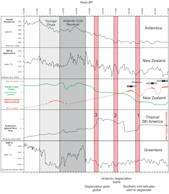
172 J. Shulmeister et al.: PEP overview 10,000 11 ,000 12,000 13,000 14,000 15,000 16,000 17,000 18,000 19,000 20,000 21,000 - 430 - 440 - 450 - 460 - 470 - 480 (delta D) Vostok Deuterium - 3.30 - 3.10 - 2.90 - 3.50 - 3.70 NW SI Speleothem (delta O)18 GISP II O 18 (delta O)18 - 3.50 - 3.60 - 3.70 - 3.80 0 - 1 1 S-America (glacial flour flux) (Petit et al. 1999) (Williams et al. 2005)

(Grootes ans Stuiver 1997) (Rodbell, unpub data)

Pukaki Crater Pollen - 1 0 1 2 (Log podocarp / grasses) ? Max. ice extent

Min. ice extent

Glacial records (New Zealand) Westland ? Younger Dryas Antarctic Cold Reversal Years BP Deglaciation goes global Antarctic deglaciation starts Southern mid-latitudes start to deglaciate Main Deglaciation complete *

3

2

1

Fig. 3. Interhemispheric timing of post-glacial warming: An alternative view. Here we summarise rock flour records from tropical South

America (Rodbell, unpublished data) and pollen (Sandiford et al., 2003), glacial (Suggate, 1990) and speleothem records (Williams et al., 2005) from New Zealand and compare them to standard deuterium records from Vostok in Antarctica (Petit et al., 1999) and the oxygen isotope ice core record from GISP II (Grootes and Stuiver, 1997). We highlight shifts in climate (Bands 1–3). Band 1 shows a shift towards warm (interglacial) conditions in New Zealand and tropical South America at about 18 500 calibrated years ago. Band 2 marks the onset of continuous warming in the Antarctic at about 17 000 calibrated years ago and Band 3 marks a second warming phase in South America and New Zealand and the first indication of warming in Greenland. In summary, these data suggest that warming initiates in the tropics and southern mid-latitudes and is transmitted to the Antarctic before warming initiates in northern high latitudes. It is recognised that some workers place NH warming much earlier (e.g. Alley et al., 2002, see text).

increases in the abundance of glacial flour. These records clearly show the initial reduction in glacial flour flux begin-ning prior to 20 000 cal yr BP, and cessation by ∼19 000 cal yr BP. Sediment records from lakes within the LGM ice limits record a late glacial readvance that was underway by 14 000 cal yr BP, and rapid ice retreat that began ∼13 000 cal yr BP (Rodbell and Seltzer, 2000). Most paleoglaciers re-treated to nearly modern (∼1950 AD) limits by 12 500 cal yr BP, but some actually disappeared for several thousand

years before reforming in the mid-late Holocene (Abbott et al., 2003).

There has been considerable disagreement over the moraine evidence for an ice advance synchronous with the YD advance of the NH (reviewed in Rodbell and Seltzer, 2000). In general, there is neither the necessary age con-trol nor the unambiguous stratigraphic evidence to provide compelling evidence for a significant ice advance during the YD in the tropical Andes. The aforementioned lake sediment

evidence, which is both well-dated and continuous, provides solid evidence for rapid ice retreat during the YD. The YD, however, was apparently cold in the tropical Andes as evi-denced by the Huascaran Peru ice core record (Thompson et al., 1995). Thus it appears that conditions must have become suddenly drier during this time in order to drive significant ice retreat.

2.1.5 Summary

The timing of the maximum glaciation in the latter part of the last ice age in the Andean tropics of South America pre-ceded the LGM by 5–10 kyr. There is widespread evidence of late OIS 3 advances in the tropics and mid-latitudes of the SH. These advances are bigger and more pervasive than the LGM advance, at least in the South American Andean trop-ics and in Australasia. A reasonable case can be made that the first step towards an interglacial climate occurred at about 18 500 cal yr BP in the southern mid-latitudes.

The available paleo-records suggest that the sequence of events for the last deglaciation could be re-interpreted as fol-lows (see Fig. 3): Tropical (and mid-latitude SH) glacial maxima were achieved 5–10 000 years before the LGM. The deglaciation in both regions effectively starts soon af-ter 28 000 years ago but is inaf-terrupted by smaller-scale re-advances during the LGM. This is some 4000 years before the maximum cooling in the NH as defined by Alley et al. (2002). In short, something caused deglaciation to start in the tropics and mid-latitude SH well before the NH reached maximum cooling (Mix et al., 2002). Alternatively, if step-wise warming is taken as the marker for the onset of deglacia-tion, SH tropical and mid-latitude regions started a drift to interglacial conditions about 18 500 years ago. This is 1500 years before the inferred warming of Antarctica at ∼17 000 years ago and more than 3000 years ahead of Greenland, which warmed abruptly after 14 700 years ago (e.g. Ras-mussen et al., 2006). In both Australasia and tropical Andean South America there are glacial fluctuations around 14 000 years ago though it is unclear whether their timing coincides. The significance of these observations is that they chal-lenge the basic assumptions of climate change on which we base our predictions of global climate response. The records could be interpreted to demonstrate that the Andean trop-ics and mid-latitude SH lead the polar regions, or they may be compatible with an NH climate lead. Our purpose, how-ever, is not to directly dispute the understanding of patterns of global change. It is to emphasise the extent of the un-certainty, given the limitations of the available paleoclimate records. It is imperative, therefore, that fundamental research into the basic patterns of long-term global change continues to be supported. There are large areas of the planet, notably Africa, the SH and large sections of the oceans where our un-derstanding of long-term climate and environmental change is inadequate. We will not be successful in predicting future

responses to climate modification if we cannot even specify the patterns of past changes.

3 Contribution 2. The recognition and definition of longer-term changes in modes of operation of climate phenomena. Case study: the Holocene evolution of ENSO and change from long frequency to biennial os-cillation ENSO dominance

The ENSO phenomenon contributes a large portion of the interannual (2–7 yr) variability in the modern climate sys-tem (Gagan et al., 2004). Work across all the PEP transects has led to the recognition that ENSO has changed markedly through time. In particular, a mid-Holocene shift or drift in ENSO activity by ∼5000 yr BP has been postulated from both modelling studies (e.g. Clement et al., 1999) and paleo-ENSO records (e.g. Shulmeister and Lees, 1995; Shulmeis-ter, 1999; Rodbell et al., 1999; Moy et al., 2002). A fur-ther intensification of ENSO is often invoked at around 3000 yr BP (e.g. Sandweiss et al., 2001; Woodroffe et al., 2003; Gagan et al., 2004). Understanding ENSO variations un-der mid-late Holocene conditions is particularly important because global sea-level and ice cover are effectively mod-ern, leaving potential forcings such as extra-tropical forcing, changes in mean temperature and the like to be examined (Diaz and Markgraf, 1992).

The following brief review of the ENSO phenomenon fol-lows Cane (2005) (Fig. 4). ENSO is an ocean-atmosphere circulation pattern in the Pacific set up by 2–7 year oscil-lations in the temperature contrast between the western and eastern tropical Pacific. This zonal temperature contrast is due to upwelling of cold water in the eastern equatorial cific, while warm surface waters in the tropical western Pa-cific are maintained by inflow from the equatorial regions under the prevailing easterly trade wind systems. The tem-perature contrast maintains the trade wind flow and pro-vides a positive feedback, the so-called “Bjerknes mecha-nism” (Cane, 2005). If the trade winds weaken, the flow collapses and ultimately reverses. The mechanism explains why the circulation breaks down (to an El Ni˜no) once cooling has started in the western Pacific but it does not provide the trigger for the switch to an El Ni˜no state. This is most proba-bly provided by wave propagation in the tropical ocean ther-mocline which is described as the delayed oscillator (Cane, 2005).

The bandwidth for modern ENSO oscillations is 2-7 years. Changes in the dominant period of ENSO variability can be identified from the analyses of instrumental records (e.g. Se-toh et al., 1999; An and Wang, 2000) as well as predicted conceptually from modelling (Lau and Sheu, 1988). It should be noted that some climatologists and oceanogra-phers (e.g. Federov and Philander, 2000) sound a warning on the existence of multiple modes of ENSO periodicities, pointing out that they may indicate changes in longer term

174 J. Shulmeister et al.: PEP overview

Figure 4. ENSO pattern (from Cane, 2005). (a) During normal conditions trade winds

drive upwelling off the South American coast and force warm surface waters from the

eastern tropical Pacific to the western Pacific. The deep pool of warm water in the

western tropical Pacific (a.k.a. West Pacific Warm Pool –WPWP) causes intense

convection over the WPWP. Rising air circulates eastward and subsides in the eastern

Pacific over the cooler upwelling water, closing the circulation loop. (b) During El Niño

events, the trade winds decline and warm water flows from the WPWP to the eastern

Pacific. The shoaling of the WPWP causes a decline in convection in the western Pacific

and a convective cell migrates eastward. This causes widespread modification of global

weather patterns. Reprinted from Earth and Planetary Science Letters, 230, M.A. Cane,

The evolution of El Niño, past and future, 227-240, 2005, with permission from

Elsevier

Fig. 4. ENSO pattern (from Cane, 2005). (a) During normal conditions trade winds drive upwelling off the South American coast and force

warm surface waters from the eastern tropical Pacific to the western Pacific. The deep pool of warm water in the western tropical Pacific (a.k.a. West Pacific Warm Pool – WPWP) causes intense convection over the WPWP. Rising air circulates eastward and subsides in the eastern Pacific over the cooler upwelling water, closing the circulation loop. (b) During El Ni˜no events, the trade winds decline and warm water flows from the WPWP to the eastern Pacific. The shoaling of the WPWP causes a decline in convection in the western Pacific and a convective cell migrates eastward. This causes widespread modification of global weather patterns. Reprinted from Cane, M. A., The evolution of El Ni˜no, past and future, Earth Planet. Sci. Lett., 230, 227–240, 2005, with permission from Elsevier.

background climatology modifying the apparent expression of ENSO rather than the phenomenon itself.

Tomita and Yasunari (1993) identified two types of ENSO; a long-frequency ENSO with a mean duration of 57 months and a biennial-oscillation ENSO with a duration of 30 months. This bi-modal ENSO of Tomita and Yasunari has not been widely recognised and the example is provided as a case study of how variable ENSO periodicities could im-pact regional climates. According to the authors the biennial-oscillation ENSO causes a sea surface temperature (SST) anomaly for only one year in the eastern tropical Pacific but is associated with a clockwise eddy of wind-stress anoma-lies in the western tropical Pacific during the “mature” El Ni˜no phase (Tomita and Yasunari, 1993). This wind stress anomaly assists in terminating the El Ni˜no phase of the ENSO phenomenon and forms part of a teleconnection to the East Asian winter monsoon. Long-frequency ENSO causes SST anomalies in the eastern equatorial Pacific for three suc-cessive years but has no wind-stress anomaly in the western tropical Pacific.

ENSO has very significant climatic impacts within the Pa-cific basin, and through teleconnections to other parts of the globe. Substantial progress has been made in understanding the modern phenomenon, but ENSO has proved very variable in both temporal and spatial impacts, and modern ocean and atmosphere records are not long enough to decipher long-term changes in ENSO behaviour. Here we present a series of ENSO records from across the South Pacific Basin. Cu-mulatively these records clearly indicate that the frequency of ENSO events has increased through the course of the Holocene and that the mean strength of El Ni˜no events has also increased. The records do not, however, imply that the ENSO system has ever switched off.

3.1 ENSO in South America

The impact of ENSO on the western margin of South Amer-ica has been documented for the past several centuries (e.g., Quinn et al., 1987). During non-El Ni˜no years in the trop-ical eastern Pacific, tradewind circulation dominates, SSTs

are cool, and the ∼75 km wide onshore coastal belt below 3000 m a.s.l. is very dry. During El Ni˜no events tradewinds slacken, the thermocline in the eastern Pacific deepens, and rainfall increases dramatically along the coast. During strong El Ni˜no years, rising motions occur in parts of the eastern Pacific troposphere that are normally characterized by subsi-dence and inversion. Under these conditions, rainfall along the coast can be extreme, driven by intraseasonal bursts of deep convection and torrential rainfall.

The inland extent of precipitation events is limited, and, generally, east of the crest of the Andes the climatic response to El Ni˜no events is muted, and in some regions the response is opposite of that noted along the coastal belt. One region where the latter is especially true is on the Peruvian-Bolivian Altiplano. In this region, El Ni˜no events are marked by a significant reduction in precipitation.

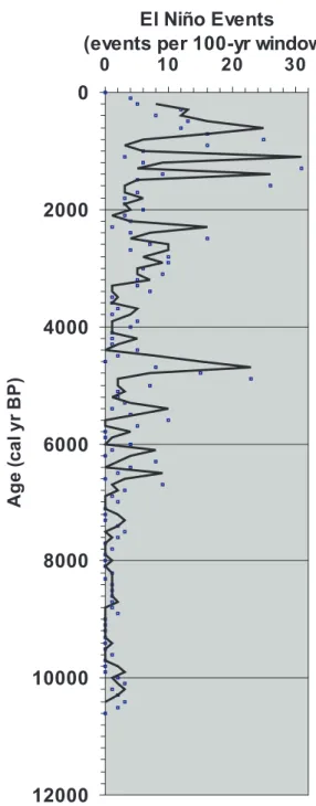
The best known record from the high Andes is the Laguna Pallcacocha (Ecuador) record (Rodbell et al., 1999; Moy et al., 2002). Here a 15 000-year record of clastic sediment in-flux to a lake marks precipitation driven run-off events in a normally semi-arid setting. Spectral analysis of colour changes in the sediments related to the influx events shows that for the last 150 years the colour banding contains signifi-cant spectral variance in the 2–7 year ENSO bandwidth. The influx bands are associated with warm SST excursions off the coast of Ecuador during El Ni˜no events. Modern ENSO band variance, along with decadal to centennial scale vari-ance, appears after about 6000 years ago.

The Laguna Pallcacocha record demonstrates a long-term drift from long period variability to shorter period variability (Fig. 5). During the early Holocene, all the spectral variabil-ity occurs at long time periods dissimilar to modern ENSO signals. From 6000 to about 3000 years ago the period of variability shortens and a ca. 7 yr ENSO signal becomes vis-ible. In the last 3000 years the signal frequency has been in-creasing and 3–4 year period signals have become important. In short ENSO frequency appears to have increased through the Holocene at this site.

A limitation of the Lake Pallcacocha record is that the banding is non-annual and the bands reflect individual sed-imentation (precipitation) events. Consequently, there is a minimum threshold that needs to be exceeded before a band will be deposited. Changes in the amplitude of ENSO events could mimic the effect of changes in periodicity, if the changes in amplitude fluctuate around the threshold value. Changes in amplitude are interpreted to be present in the record.

Over the last 6000 years, where ENSO has been visible in this record, it is not consistently strongly “on”. Instead at least three phases of enhanced ENSO events centred around 5000, 3000 and 1000 years ago can be recognised. This was inferred by Moy et al. (2002) to represent a roughly 2100 year cyclicity. This repetitive pattern may be forced by inso-lation (solar activity).

0

2000

4000

6000

8000

10000

12000

0

10

20

30

El Niño Events

(events per 100-yr window)

A

g

e

(cal

yr

B

P

)

Fig. 5. Number of strong El Ni˜no events recorded in Laguna

Pall-cacocha Ecuador per 100 year overlapping window (from Moy et al., 2002). The early Holocene was marked by fewer events and the frequency of events increased through the Holocene beginning

∼6000 cal yr BP and peaked several times in the last 2000 yr.

Recently, the first nearly-continuous 20,000-year long archive of past El Ni˜no activity has been obtained from ma-rine sediments off the coast of Peru (Rein et al., 2005). This record shows significant El Ni˜no activity as early as 17 000 cal yr BP, strong activity during the late glacial, and a marked reduction in El Ni˜no activity from 9–5000 years BP. The Holocene portion of this record agrees well with the

176 J. Shulmeister et al.: PEP overview

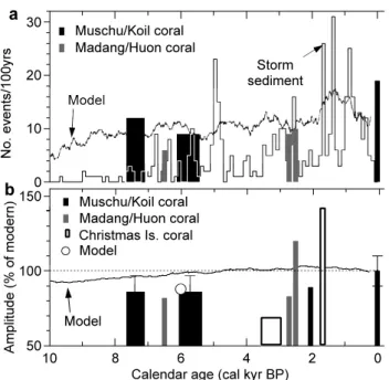
Fig. 6. From McGregor and Gagan (2004) (a) Changes in El Ni˜no

frequency given by coral δ18O records from Muschu Island, Koil Is-land, and Madang, PNG (Tudhope et al., 2001), lacustrine storm de-posits (Moy et al., 2002), and model results (Clement et al., 2000). Data are scaled to events/century to facilitate direct comparison. (b) Changes in El Ni˜no amplitude given by coral δ18O records in panel (a), the standard deviation of coral δ18O in microatolls from the cen-tral equatorial Pacific (Woodroffe et al., 2003), and model results (Clement et al., 2000; Liu et al., 2000). The threshold amplitude analysis of the Tudhope et al. (2001) coral records is restricted to El Ni˜no events to facilitate comparison with other records. Error bar for the modern Muschu Island coral record is the standard error of the mean for all El Ni˜no events recorded for 1950–1997. Errors for fossil coral percentage changes include the standard errors for both the modern and fossil corals. Reprinted with permission from Mc-Gregor, H. V. and Gagan, M. K., Western Pacific coral δ18O records of anomalous Holocene variability in the El Ni˜no-Southern Oscilla-tion, Geophys. Res. Lett., 31, L11204, 1–4, 2004, Copyright 2004 AGU.

aforementioned Pallcacocha record, however this is the first evidence of strong El Ni˜no activity during MIS 2 from the eastern tropical Pacific.

3.2 Coral records of ENSO in the West Pacific Warm Pool Viewed as an oceanic system, the Western Pacific Warm Pool (WPWP) and Indonesia form the “down-drift” core region for ENSO. Under normal conditions, the surface waters of the WPWP are very warm (>28◦C) and provide vast quan-tities of atmospheric water vapour and latent heat that drive the world’s climate. The resulting high levels of convective rainfall make the surface waters of the WPWP less saline than average tropical seawater. This low density warm pool water is displaced eastward during El Ni˜no events and SSTs in the WPWP decline by about 1◦C, mainly in response to

the thinning of the surface mixed layer and greater mixing with underlying, cooler water. Consequently, atmospheric convection in the WPWP region is disrupted during El Ni˜no events (Rasmusson and Carpenter, 1982) causing drought conditions in the WPWP region (Ropelewski and Halpert, 1987).

El Ni˜no events are recorded by massive, long-lived corals in the WPWP region through changes in the δ18O values in their skeletons. These changes in skeletal δ18O reflect the combined effect of cooler SSTs and the reduction in18 O-depleted rainfall during El Ni˜nos. Analysis of fossil corals from northern Papua New Guinea dating to 7600–5400 years years ago suggests that ENSO amplitude was reduced to 85– 40% of modern (Tudhope et al., 2001; McGregor and Gagan, 2004; Fig. 6). Records from Christmas Island in the central equatorial Pacific also contain a strong ENSO signal indi-cating ENSO amplitudes 80–60% of modern from ∼4000 to 3300 years ago (Woodroffe and Gagan, 2000; Woodroffe et al., 2003). In contrast, large and protracted El Ni˜no events are identified for 2500–1700 years ago (McGregor and Gagan, 2004) and remained above modern until the last 1000 years (Moy et al., 2002).

Analysis of individual ENSO events reveals that the pre-cipitation response to El Ni˜no temperature anomalies was subdued in the mid-Holocene (Gagan et al., 2004). There-fore, while ENSO strength may be reduced in the early Holocene, there is no suggestion from coral records for the WPWP that ENSO is eliminated. In fact, coral records doc-umenting the early Holocene climate in Indonesia (Gagan et al., unpublished data) show clear seasonal ENSO SST sig-nals, and in terms of temperature, mid-Holocene El Ni˜nos on the Great Barrier Reef were similar in amplitude to recent events (Gagan et al., 2004). Unlike recent events, however, summer rainfall was only marginally reduced, producing a record with much less interannual rainfall variability.

The relative failure of the precipitation anomaly to de-velop in these WPWP records may explain the absence of ENSO signals in Ecuador during the early Holocene. With strong convection still occurring over the WPWP, the Walker and Hadley circulations were probably still operating in their usual meridional positions, even if somewhat reduced. Therefore, the opportunity for a strong convective cell to de-velop in the eastern Pacific may have been reduced. Alter-natively, El Ni˜no-driven precipitation only reaches Lake Pal-cacocha during strong-very strong events when convection reaches ∼4000 m and the absence of El Ni˜no signals at this site during the early Holocene may indicate the absence of such strong events.

Just as the amplitude of ENSO varied through the Holocene, so too did the frequency. Unlike Laguna Pallca-cocha, where ENSO bandwidths are effectively absent until about 6000 years ago, ENSO-like phenomena are in place at 12 000 years ago elsewhere in the tropics (Rein et al., 2005). By 10 000 years ago the spectral signal shows strong forcing at 1.5–3 year bandwidths. During the peak ENSO

frequency period (about 2000 to 1000 years ago) the fre-quency of events becomes nearly annual before dropping back to a 1.5 yr bandwidth in the last millennium. The over-all frequency of events observed in coral records from the WPWP is much greater than in Ecuador, but the trend to-wards high frequency oscillation is similar. The difference between the records may again be that the Ecuador lake sediments only record El Ni˜no events when they are strong enough to trigger a rainfall anomaly in western tropical South America.

3.3 ENSO teleconnections in the SW Pacific (New Zealand)

ENSO is the principle EOF in most analyses of the New Zealand inter-annual climate. The climatic effects of ENSO were mapped in some detail by Gordon (1985) who demon-strated that the impacts in New Zealand vary by season and locality. Also, Mullan (1995) demonstrated that the effects were partially non-stationary and consequently impacts may vary through time. Despite these riders, the strong topo-graphic division of New Zealand makes regional precipita-tion signals highly sensitive to small-scale synoptic changes and these are what allow us to recognise ENSO effects. The primary ENSO impacts in New Zealand are related to the waxing and waning of surface pressure over eastern Aus-tralia in response to El Ni˜no events. During El Ni˜no events, anomalous high pressure over eastern Australia causes an acceleration of the regional southwest air-flow over New Zealand. By contrast, reduced zonal flow and more frequent development of blocking highs over the country occurs dur-ing La Ninas. Within New Zealand the northern part of North Island is particularly responsive to changes in the South-ern Oscillation (SO). Auckland and the surrounding regions have significant SO correlations (p<0.05) for temperature in Spring, Summer and Winter and for rainfall in Spring and Summer (Gordon, 1986). It just misses significance in Win-ter. The regional climate of Auckland is dominated by SW flows and the pressure anomaly maps (Fig. 11 in Gordon, 1986) highlight the susceptibility of this flow to SO varia-tions.

In the following sections we examine the impact of ENSO on the Holocene glacial records in New Zealand and on pale-oclimate records from a maar in the Auckland region. These data are then compared to the recently developed regional composite speleothem record of Williams et al. (2005). 3.3.1 Records of glacial activity and speleothems

It has been demonstrated that the strength and pattern of westerly wind flow and concomitant precipitation and cloud cover are critical to modern glacier mass balance in New Zealand (Fitzharris et al., 1992; Tyson et al., 1997; Hooker and Fitzharris, 1999). Changes in westerly air-flow can be directly correlated with ENSO and, at least for the west coast

glaciers, a prima facie relationship between a westerly index and glacier fluctuation has been established. Specifically, the modern west coast glaciers respond with a 5–7 year lag to average seasonal synoptic conditions, with advances occur-ring after years of positive zonal (southwesterly) flow and re-treats associated with years of meridional (northerly) anoma-lies. East coast glaciers, on the other hand, have longer re-sponse times and respond to longer period (decadal) forc-ing. Millennial-scale changes in the westerlies will be con-trolled by the pole-equator temperature gradient, which is most likely driven by orbital forcing through modification of insolation derived seasonality (e.g. Dodson, 1998; Shulmeis-ter, 1999; Shulmeister et al., 2004).

The long-term records from these glaciers indicate a re-markable absence of evidence for glacial advances from 9000 to 5000 years ago. After 5000 years the glacial sys-tems switched on. The best-studied Holocene glacial record comes from the west coast, Franz Josef Glacier, which ad-vanced at 5000, 2500, 1500 years ago and during the Little Ice Age (Wardle, 1973). This suggests ENSO activity has stepped-up in the latter half of the Holocene.

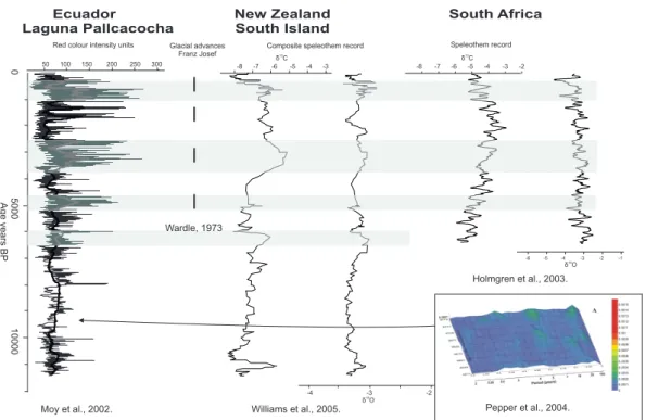
Until recently, there was no long-term continuous record to compare with the intermittent glacial record. The compila-tion of a composite speleothem stable isotope record for New Zealand (Williams et al., 2005) provides one. In Fig. 7, this speleothem record is plotted against the Franz Josef glacial record, the colour spectral signal of ENSO from Laguna Pall-cacocha (Moy et al., 2002) and, as an independent check, against a composite speleothem record from South Africa (a SH site that is affected by, but not a core region for, ENSO impacts). The comparison supports the coherence of paleo-ENSO records for New Zealand and South America through the Holocene. In both Laguna Pallcacocha and New Zealand, the earliest flickering of a signal of greater variability occurs about 6000 years ago and the systems swing strongly to a new (ENSO) mode after 5000 years ago. In contrast, the South African record shows very little similarity to Laguna Pallcacocha and New Zealand.

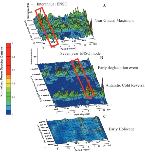
Thus far, nothing in the New Zealand record gives in-sight into changes in ENSO frequency. We cannot demon-strate a Holocene change in bandwidth from New Zealand, but we can demonstrate that ENSO operated differently dur-ing the LGM and deglaciation. Laminated sediment records from Auckland Maar craters are the key (e.g. Horrocks et al., 2005). Some of these laminae are at least quasi-annual and, as they are largely organic, they are measures of primary pro-ductivity. The laminae become thinner from the LGM to the Holocene, so they cannot be driven by either temperature or insolation (Pepper et al., 2004) (Fig. 8). Instead, nutrient lim-itation is the likely driver because the maar lakes are small, deep, closed basins without catchments, so fluvial activity is minimal. The only likely source of variable nutrients is via aeolian input. Both dry and wet deposition are possible but, given that the regional dominant wind (SW) is also the major rain-bearing wind, the sources for both wet and dry

178 J. Shulmeister et al.: PEP overview 0 Age years BP 5000 10000 -8 -7 -6 -5 -4 -3 -8 -7 -6 -5 -4 -3 -2

Ecuador New Zealand South Africa

Laguna Pallcacocha South Island

-6 -5 -4 -3 -2 -1 ä O18 -4 -3 -2 ä O18 ä C13 ä C13 50 100 150 200 250 300

Red colour intensity units Glacial advances Composite speleothem record Franz Josef Speleothem record Holmgren et al., 2003. Pepper et al., 2004. Williams et al., 2005. Wardle, 1973 Moy et al., 2002.

Fig. 7. Comparison between the Holocene ENSO records from Laguna Pallcacocha in Equador (Moy et al., 2002), New Zealand glaciers

(Wardle, 1973) and speleothem records (Williams et al., 2005) and South African speleothem records (Holmgren et al., 2003) for the Holocene. Gray bars have been used to highlight apparent periods of strong ENSO activity in the Ecuador and New Zealand records. These suggest strong coherence between the South American and New Zealand records and a stronger but distinctly episodic ENSO signals in the last ca. 5000 years. South Africa shows little coherence. A short early Holocene record from Auckland Maar Lakes (Pepper et al., 2004) is inset. This record shows no spectral power in ENSO time domains. It confirms the weak teleconnections to New Zealand at this time.

Va r ia t ion of la mina e down c or e

0.00 0.20 0.40 0.60 0.80 1.00 1.20 1.40 1.60 Laminae Thickness (mm) 0 200 400 800 1000 1200 1400 1600 1800 2000 2200 2400 2600 2800 600 Number of Laminae Thin section of laminae Deglaciation segment Pre-LGM segment

Antarctic Cold Reversal Early Holocene segment 1 mm From Pepper 2003 300 km New Zealand Onepoto maar

b

a

c

Fig. 8. After Pepper (2003). Laminated lake sediments in thin section (a) from Onepoto Maar (b) in Auckland. Graph (c) displays laminae

thickness for three selected periods in early Holocene, the Last Glacial Interglacial Transition and just prior to the LGM. The laminae are generally thicker during the last glaciation than during the Holocene. The laminae are largely biological (algal) in origin and reflect quasi-annual to quasi-annual productivity in the Maar. These records display a general pattern of declining lamina thickness from the LGM to the Holocene but with two periods of greatly enhanced laminae (= productivity) during the deglaciation. This is believed to reflect increased wet and dry deposition of dust under zonal SW winds at this time.

0 0.2 0.4 0.6 0.8 1 Period (years) 2 2.5 3 4 5 7 10 20 100

B

A

C

Antarctic Cold Reversal

Early deglaciation event

Near Glacial Maximum

Interannual ENSO

Seven year ENSO mode

Early Holocene

Fig. 9. Spectral analyses of lamina thickness from Onepoto Maar during parts of (a) immediately prior to the LGM (b) the deglaciation and (c) the early Holocene. The deglacial section displays a 7 year ENSO like periodicity during two distinct episodes, which coincide with the

sections of thickened laminae in Fig. 7. The younger of these matches the onset of the Antarctic Cold Reversal (ACR). The ACR appears to be reflected in New Zealand by a strengthening of the regional SW flow which amplifies the ENSO signal enough for it to be reflected in the record. Reprinted with permission from Pepper, A. C., Shulmeister, J., Nobes, D. C., and Augustinus, P. C., Possible ENSO signals prior to the last Glacial Maximum, during the deglaciation and the early Holocene from New Zealand, Geophys. Res. Lett., 31, L15206 1–4, 2004, Copyright 2004 AGU.

deposition coincide. Therefore, we interpret these records to show variability in the southwest wind which, in the Auck-land region, is strongly related to ENSO variability (Gordon, 1985). The Auckland Maar record shows strong coherence at a 2–3 year bandwidth near the LGM. There is no visible ENSO signal in the early Holocene, but during the deglacia-tion there are two brief periods showing strong spectral forc-ing at a 7 year bandwidth (Fig. 9).

3.4 Discussion/Summary: Changes in the amplitude and frequency of ENSO events

ENSO switches up and down (rather than on and off) dur-ing the Holocene. Clearly, there are important changes in paleo-ENSO dynamics in the middle Holocene. To in-terpret the Holocene evolution of ENSO, we lean towards the hypothesis of Haug et al. (2001) who suggested that the ITCZ was located further north during the early-middle Holocene. This may have strengthened the links between ENSO and the NH monsoonal systems but weakened the

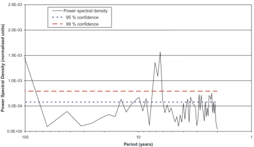
180 J. Shulmeister et al.: PEP overview Significant Peaks in PSD 0.0E+00 5.0E-04 1.0E-03 1.5E-03 2.0E-03 2.5E-03 1 10 100 Period (years) P o w e r S p ect ra l D en sity (n or ma lised un its )

Power spectral density 95 % confidence 99 % confidence

Fig. 10. Statistical significance of PSD peaks in the time period of the Antarctic Cold Reversal. The 5–7 year peaks are significant at 3 σ

and there are significant peaks in interannual and decadal periods at 2 σ . The peak near the 100 year period is an edge effect (see Pepper et al., 2004).

link between the Southern Oscillation and ITCZ rainfall pat-terns in the southern tropics. This would allow the oceanic ENSO temperature signal to be maintained through the early Holocene, as indicated by coral records in the WPWP, in the absence of detectable rainfall anomalies in Ecuador and New Zealand. After 5000 years ago, and especially after 3000 years ago, strengthening links between a southward drifting ITCZ and the Southern Oscillation established the modern rainfall anomalies.

The second half of the Holocene is clearly a period of en-hanced ENSO variability, but it is not uniformly enen-hanced. A critical feature of the Laguna Pallcacocha and New Zealand records is that they suggest phases of enhanced ENSO activ-ity that extend for at least several hundred years, which are separated from each other by hundreds to thousands of years. The evidence from the WPWP shows that ENSO is likely to have been active at inter-annual bandwidth, if at somewhat reduced amplitude, through the entire period. The implica-tion is that transmission of ENSO signals, even to the proxi-mal tropical coast of western South America, requires more than the ENSO oscillation itself.

We conclude that the frequency patterns visible in sites connected by rainfall anomaly teleconnections may not re-flect true ENSO base frequencies. While the records indi-cate that El Ni˜no events became stronger and more frequent through the Holocene, it is likely that they reflect the inci-dence of extreme events within the ENSO cycles. Never-theless, they represent a real shift towards shorter frequency El Ni˜nos. The pattern is important because bi- or multi-modal oscillations are discernable in the modern ENSO cy-cle. These modes have similar but not identical climatologies and a systematic shift in the frequency means a systematic

shift in climatological responses. It is important because the mode helps to indicate which teleconnections are likely to operate. This will allow us to both better predict the nature of ENSO events themselves and the long-distance climate impacts.

We propose that the strengthened ENSO regime of the late Holocene is a function of a strong SH seasonality that en-hances zonal circulations in the SH and reinforces the South-ern Oscillation. This sets up the conditions for both increased ENSO amplitude and increased ENSO frequency. Therefore, it is probably not accidental that the most extreme period of ENSO activity (∼2500–1500 years ago) coincides with max-imum SH seasonality.

4 Contribution 3: The recognition of climate modula-tion of oscillatory systems by climate events. Interac-tions between climate phenomena and climate events – the case of the Antarctic Cold Reversal

Human systems are capable of dealing with gradual environ-mental drift but a rapid change, even of relatively small mag-nitude, can cause extreme hardship and potentially system collapse. This can be observed on all time scales. For ex-ample, the Tambora eruption of 1815, which created the so-called “year without a summer”, disrupted agriculture across much of the globe and caused famines in Europe and else-where (Strothers, 1984). The implications of a major abrupt change, such as the shut-down of the global thermohaline cir-culation that has recently caught the popular imagination, are widespread and potentially catastrophic for human societies. Unlike gradual climate drift, which can be modelled with General Circulation Models (GCMs) using standard flux

equations and modern boundary conditions, changes in sys-tem mode will not (normally) fall out of climate models. The only real strategy to predict mode changes is to examine the history of climate systems from the paleo-record, to see whether and how the system has behaved in the recent geo-logical past. Some syatem changes over the last 20 000 years are now becoming well recognized, in particular the late-last glaciation abrupt cooling known as the Younger Dryas, and oscillatory changes such as Dansgaard-Oescher events. Recognition of these events allows us to estimate the direc-tion and extent of change possible in climate systems. It also may allow us to identify the trigger, which gives us the po-tential for managing some of the changes. As the quality and density of paleo-records improves we are also beginning to recognise the global teleconnections linked to climate change events and can make useful, if still unquantified statements about far-field effects of change. Here we present one ex-ample, the Antarctic Cold Reversal (ACR) where the climate link between a change in one region (coastal Antarctica) and its effect in another (New Zealand) can be demonstrated. 4.1 The Antarctic Cold Reversal in the New Zealand record In Sect. 2.3.2 we highlighted a maar lake record from the Auckland region, New Zealand, that demonstrates strong ENSO-like periodicities (Pepper et al., 2004). Within that record the transition from the last glaciation to the present in-terglaciation presents a clear story. For most of the deglacia-tion, there is no evidence of strong inter-annual variability in the Auckland region. During two brief interludes, how-ever, strong inter-annual variability at a 7 year ENSO pe-riodicity is observed and is statistically significant (Fig. 10). The younger of these two events aligns well with the onset of the Antarctic Cold Reversal between 14 800 and 14 500 years ago (Jouzel et al., 1995; Blunier et al., 1997). The duration of the event is much shorter than the ACR, lasting about 150 years as opposed to the 1700 years of the ACR. Neverthe-less the coincidence of the timing of initiation is compelling. Furthermore, there is a strong ACR record from the ocean off New Zealand (Carter et al., 2003) and it shows up in terrestrial paleoecological records (e.g. Turney et al., 2003; McGlone et al., 2004).

The ACR manifests itself in Antarctica as a cool anomaly recorded in the oxygen isotope ratios of ice formed at ∼14 800 years ago. Simplistically, a decrease in tempera-tures in the Antarctic margin would be expected to increase the speed of the zonal westerlies to the north by increasing the thermal (pressure) contrast between the polar region and the surrounding ocean. A general increase in westerly cir-culation at southern mid-latitudes would be expected. This is observed from the Auckland record. The individual lami-nae in the maar records are interpreted as annual and reflect aeolian flux to the maar under zonal south-westerly flows. During the ACR event the laminae are significantly thicker than at any other time since the LGM (Fig. 8). In short the

general pattern of the Auckland record is compatible with a simplistic predicted change in westerly wind strength under Antarctic cooling.

The additional factor is the apparent enhancement of an ENSO signal in the New Zealand region during this event. ENSO has been identified as an important driver of Antarctic climate change on inter-annual to decadal scales (e.g. Kwok and Comiso, 2002). Under modern conditions, ENSO tele-connections exist between New Zealand and the Antarc-tic. Links between ENSO warm events in the South Pa-cific and impacts in Antarctica have been recognised, partly through the mechanism of blocking highs hindering migra-tion of the Amundsen Sea Low (Renwick, 1998; Bertler et al., 2004). The connections are also interlinked with vari-ability in the Antarctic Oscillation (e.g. Fogt and Bromwich, 2006; L’Heureux and Thompson, 2006). The position (or ab-sence) of blocking systems in the South Pacific and eastern Australia, in turn, control the zonal flows over New Zealand during ENSO events (and at other times). This relationship is, however, both seasonal and non-stationary. In the Ross Sea, the regional climate shows a significant positive ENSO correlation during the last decade whereas no significant cor-relation is observed in the decade from 1971–1980 (Bertler et al., 2004).

Since the Antarctic is not the source area for ENSO, we do not suggest that ENSO actually switches on during the ACR. Rather, we infer that circulation changes associated with the ACR event amplified an existing ENSO signal in the New Zealand region. This occurred through an enhancement of zonal wind flows that magnified the signal sufficiently for it to become visible through primary production in the Auck-land maar.

This type of study provides insight into the climatology of a teleconnection for a climate change event. The El Ni˜no-style anomaly can be projected out of the NZ region using modern climatologies to provide a testable prediction of re-gional responses to the ACR. These predictions can be tested by further paleoclimate studies in other regions. However, it is likely that only high temporal resolution paleoclimate re-search will be capable of providing insights into how global climate change is transmitted.

5 Conclusions

The PEP projects of PANASH have extended our understand-ing of past climate change. The main messages from this paper are:

1) Low resolution records provide information on chang-ing background states on which ENSO, the monsoons and other climate phenomena are superimposed. This is a criti-cal underpinning for the higher resolution studies. In addi-tion, as we move towards higher precision, numerical, recon-structions of climate parameters we need the verification that broad reconstructions provide. Many of these low resolution

182 J. Shulmeister et al.: PEP overview records provide a higher reliability than the numerical

re-constructions. The presence of tree stumps in growth po-sition, for example, guarantees that local conditions were favourable enough for trees to grow. Such high reliability indicators greatly reinforce the inferences from numerical re-constructions.

The need for ongoing basic research is highlighted by the fact that although very significant advances have been made in the understanding of past climate systems, we cannot yet define the basic patterns of past climate change accurately. We cannot even hope to reconstruct global impacts of cli-mate change if we have very intermittent coverage of the globe. We note particular data deficiencies over much of the SH, the oceans and Africa. We have highlighted this predica-ment by demonstrating that one of the better studied periods, the transition from the Last Glaciation Maximum to the cur-rent Interglaciation can be re-interpreted in the light of recent paleo-climate finds. We cannot even specify with confidence whether the post LGM warming initiates at one of the Poles or the equator.

2) There is a real need for annually resolved paleoclimate records. This paper has highlighted the rapid growth in our understanding of the geological history of ENSO. The stud-ies that have provided this insight are annual in resolution, or higher, because only these studies can examine the phe-nomenon. In fact, the increase in understanding reduces our ability to make simple statements about the phenomenon. It is our view that the core ENSO system probably operates continuously through the Holocene but that teleconnections through precipitation and other anomalies are non-stationary on centennial and millennial scales. Major changes in cli-mate can occur without ENSO switching on or off. The change in frequency and the possible relationship of this change to insolation forcing is also important, both because it affects regional climate responses and because the geo-logical observations allow models of climate change to be tested against real data. The better we know the history of the climate systems, the better our hope of predicting cli-mate change and subsequently managing environmental con-sequences.

With respect to annual records, bioturbation of sea-floor sediments is a particular problem. While in earlier stud-ies the relatively high resolution (centennial scale) from ma-rine cores gave a comparative advantage over the available discontinuous terrestrial records, the situation is slowly re-versing. Ice core, laminated lake, dendro- and speleothem records all allow quasi-annual resolution on land. We need annual resolution to examine climatic phenomena, such as ENSO, which cannot be examined in centennial resolution records. There is an urgent need to identify higher resolu-tion marine records that can actually see these signals. Other than coral proxies, only a handful of records from anoxic sites (e.g. Rein et al., 2005) can actually be used to examine these types of change.

3) “Rates of change” is one of the critical pieces of the jig-saw that paleoclimate studies can provide. The risk of abrupt climate change is recognised as very important and inher-ently difficult for future climate change prediction (Watson et al., 2001). Human systems are quite adaptable to change so long as it is gradual and predictable. The same systems may collapse under even moderate change scenarios if the rate of change is too great. Paleoclimate work is the only reliable tool to evaluate how fast natural systems can change. The observation of interactions between abrupt climate phenomena and oscillatory systems requires well-dated high resolution paleoclimatic records. Thus far paleoclimate work has allowed us to recognise that abrupt climate changes have occurred and to specify some aspects of the change in the core affected regions. Paleoclimate work needs to extend to examining the teleconnections between the abrupt phe-nomena and distal climates. The importance of distal re-sponses to abrupt change has been recognised for some time (e.g. Broecker, 2000) but it is only with the proliferation of quasi-annual resolution records that we can start to recognise the climatic processes involved in the teleconnections them-selves.

4) Modelling work provides the global view and improves our understanding by giving insights into the processes con-trolling climate change. Paleo-data provide both verification for model runs and in some instances the data and ideas to generate the model scenarios. Modelling provide us with the dynamic reconstructions of past climates and the ability to examine teleconnections. It gives us the ability to turn re-constructions of local climates into powerful tools for pre-dicting future climate change and managing environmental consequences.

Acknowledgements. We dedicate this paper to the memory our

colleague and friend G. O. Seltzer, long-time leader of the PEPI project and a major player in much of the science presented in this paper. J. Shulmeister acknowledges Marsden Grant UOC301 and University of Canterbury internal grant U6508 for support of glacial work and PGSF grant VIC-009 for paleolimnological investigations. He thanks the Department of Geosciences, Idaho State University and the RMAP programme RSPAS, Australian National University for hospitality and facilities while writing this paper during a sabbatical visit. D. Rodbell acknowledges NSF grants EAR9418886 and ATM-9809229 for support of his work in the tropical Andes. M. K. Gagan acknowledges Australian Research Council grant DP0342917 for support of his work in the west Pacific Warm Pool region. We thank D. Nobes for help with the Onepoto spectral analyses and the anonymous referees for their comments that have resulted in a significantly tightened final manuscript.

Edited by: T. Kiefer

References

Abbott, M. B., Wolfe, B. B., Wolfe, A. P., Seltzer, G. O., Ar-avena, R., Mark, B. G., Polissar, P. J., Rodbell, D. T., Rowe,