HAL Id: hal-02396900
https://hal.archives-ouvertes.fr/hal-02396900
Submitted on 6 Dec 2019
HAL is a multi-disciplinary open access
archive for the deposit and dissemination of
sci-entific research documents, whether they are
pub-lished or not. The documents may come from
teaching and research institutions in France or
abroad, or from public or private research centers.
L’archive ouverte pluridisciplinaire HAL, est
destinée au dépôt et à la diffusion de documents
scientifiques de niveau recherche, publiés ou non,
émanant des établissements d’enseignement et de
recherche français ou étrangers, des laboratoires
publics ou privés.
Transition prediction on Reentry-F trajectory with PSE
at chemical equilibrium
Jean-Philippe Brazier, Jean Perraud, Jacques Couzi
To cite this version:
Jean-Philippe Brazier, Jean Perraud, Jacques Couzi. Transition prediction on Reentry-F trajectory
with PSE at chemical equilibrium. FAR 2019, Sep 2019, MONOPOLI, Italy. �hal-02396900�
TRANSITION PREDICTION ON REENTRY-F TRAJECTORY
WITH PSE AT CHEMICAL EQUILIBRIUM
Jean-Philippe Brazier
(1), Jean Perraud
(1), Jacques Couzi
(2)(1)
ONERA/DMPE, Université de Toulouse, France,
Jean-Philippe.Brazier@onera.fr
(2)
CEA CESTA, Le Barp, France,
Jacques.Couzi@cea.fr
ABSTRACT
The laminar-turbulent transition is a key feature of hypersonic flows on reentry vehicles. For a smooth wall, its position can be estimated by a stability analysis of the boundary-layer, using the Local Stability Theory (LST) or the Parabolized Stability Equations (PSE). These techniques have been applied to the trajectory of Reentry-F flight experiment, assuming an axisymmetric flow and air at thermochemical equilibrium. The results have been compared with experimental data and results from previous published works. The transition is found to move gradually closer to the nose when the altitude decreases and the Reynolds number increases.
Index Terms — Laminar-turbulent transition, hypersonic flows, boundary-layer stability, chemical equilibrium, PSE, Reentry-F
1. INTRODUCTION
Predicting the laminar-turbulent transition is a key issue for hypersonic reentry vehicles, since the occurrence of turbulent flow induces a dramatic increase of the wall heat flux, which must be taken into account for the design of the thermal protection. For a smooth wall, the transition is commonly triggered by the linear amplification of initially small perturbations, due to the intrinsic instability of the boundary layer. When the amplitude of the fluctuations reaches a sufficient level, nonlinear interactions occur, giving rise to chaotic phenomena and turbulence onset. A detailed description of boundary-layer linear stability theory has been given by Mack [1]. The most common approach to compute boundary-layer stability is the Local Stability Theory (LST). An improved theory, called Parabolized Stability Equations (PSE) has also been proposed by Herbert [2]. Both methods will be briefly explained in §2.
A particular aspect of reentry flows is that due to the very high velocities, the stagnation temperature reaches high values such that dissociation effects occur in the air, which can no longer be considered as a perfect gas. Thermochemical nonequilibrium may be observed in such
flows. In the present work, as a first step, only chemical equilibrium is addressed and air properties are interpolated in a Mollier diagram.
In order to evaluate the efficiency of these methods, they have been both applied to the sphere-cone used for the Reentry-F flight experiment, which took place in 1968 in the USA [3,4], for five points of the trajectory. This experiment was used as test case in several previous works [5-9]. The flight parameters are reminded in §3, together with information on the computation of the mean flow. The present stability results computed at the five selected altitudes are presented in §4 and compared with flight data and previous results.
2. PRINCIPLE OF STABILITY ANALYSIS
All the usual methods used to compute the instability of the boundary layer rely upon the difference of length scale along the flow and along the normal to the wall. Whereas the flow undergoes a fast variation across the boundary-layer thickness, it varies slowly in the streamwise direction, as long as the wall geometry is smooth and exhibits a curvature radius very large with regard to the boundary-layer thickness. The evolution of a small perturbation of a given mean flow is thus described by the linearized Navier-Stokes equations, where further simplifications are introduced by the method of multiple scales, to take into account the slow streamwise variation of the mean flow. In the present work, only axisymmetric flows will be addressed.
First, the following decomposition is applied to all the variables of the unsteady flow, where 𝜉𝜉 and 𝜂𝜂 represent respectively the streamwise and wall-normal coordinates, 𝑞𝑞� represents the steady mean flow, 𝑞𝑞′ the perturbation, and 𝜀𝜀 an arbitrary small parameter:
𝑞𝑞(𝜉𝜉, 𝜂𝜂, 𝑡𝑡) = 𝑞𝑞�(𝜉𝜉, 𝜂𝜂) + 𝜀𝜀𝑞𝑞′(𝜉𝜉, 𝜂𝜂, 𝑡𝑡)
2.1. Local stability theory (LST)
In this approach, only the dominant terms are retained in the perturbation equations. The mean flow is therefore supposed
to be locally invariant in the streamwise direction and Fourier transforms can be applied in both longitudinal and temporal directions. The perturbation can be expressed under the following form of a normal mode:
𝑞𝑞′(𝜉𝜉, 𝜂𝜂, 𝑡𝑡) = 𝑞𝑞�(𝜂𝜂)𝑒𝑒𝑖𝑖(𝛼𝛼𝛼𝛼−𝜔𝜔𝜔𝜔)
where ω is real and corresponds to the fixed angular frequency, whereas the streamwise wave number α is complex. The η-derivatives are expressed with a discretization scheme and the linear perturbation equations can be put under a generalized eigenvalue problem for α:
𝐴𝐴𝐴𝐴 = 𝛼𝛼𝛼𝛼𝐴𝐴
where X is the vector of all 𝑞𝑞� and the matrices A and B depend on ω and on the local mean flow field. When the imaginary part of the eigenvalue α is positive, the wave is damped, but when it is negative, the wave is amplified and the flow is convectively unstable.
2.2. Parabolized stability equations (PSE)
The PSE are derived following a similar approach but retaining dominant and first order terms. They should be more accurate since they include terms related to the axial variation of the mean flow and to the wall curvature. The perturbation reads now:
𝑞𝑞′(𝜉𝜉, 𝜂𝜂, 𝑡𝑡) = 𝑞𝑞�(𝜉𝜉, 𝜂𝜂)𝑒𝑒𝑖𝑖(𝜑𝜑(𝛼𝛼)−𝜔𝜔𝜔𝜔)
with
𝜑𝜑(𝜉𝜉) = � 𝛼𝛼(𝑥𝑥)𝑑𝑑𝑥𝑥𝛼𝛼
0
The ξ coordinate now appears twice. The phase function
φ(ξ) contains the fast axial variation of the perturbation,
related to the wave length, whereas the amplitude function 𝑞𝑞� represents the slow variation due to the axial gradient of the mean flow. A normalization condition such as
� 𝑞𝑞�𝛿𝛿 ∗ 0
𝜕𝜕𝑞𝑞�
𝜕𝜕𝜉𝜉 𝑑𝑑𝜂𝜂 = 0
associated to an iteration on α must be added to close the system [2]. The PSE are no longer an eigenvalue problem but evolution equations that read under matrix form
𝑀𝑀12 𝜕𝜕 2𝐴𝐴 𝜕𝜕𝜉𝜉𝜕𝜕𝜂𝜂 + 𝑀𝑀22 𝜕𝜕2𝐴𝐴 𝜕𝜕𝜂𝜂2 +(𝑀𝑀1+ 𝑖𝑖𝛼𝛼𝑄𝑄1)𝜕𝜕𝐴𝐴𝜕𝜕𝜉𝜉 +(𝑀𝑀2+ 𝑖𝑖𝛼𝛼𝑄𝑄2)𝜕𝜕𝐴𝐴𝜕𝜕𝜂𝜂 + �𝐴𝐴0+ 𝑖𝑖𝑖𝑖𝐴𝐴1+ 𝑖𝑖𝑑𝑑𝛼𝛼𝑑𝑑𝜉𝜉 𝐴𝐴2+ 𝑖𝑖𝛼𝛼𝐴𝐴3+ 𝛼𝛼2𝐴𝐴4� 𝐴𝐴 = 0
Since the amplitude functions exhibit slow evolution in the axial direction, the PSE can be solved by space marching with a large step size, in spite of the fact that they are not exactly parabolic. As usual, a very accurate discretization scheme is needed for η-derivatives whereas a simple first-order implicit backward Euler scheme is used for forward marching.
2.3. Transition prediction
From the local stability theory, the local amplitude A(ξ) can be deduced as
𝐴𝐴(𝜉𝜉) = 𝐴𝐴0� −Im[𝛼𝛼(𝑥𝑥)]𝑑𝑑𝑥𝑥 𝛼𝛼
𝛼𝛼0
where A0 is the initial amplitude and ξ0 is the abscissa where
the wave becomes unstable at the prescribed frequency. For PSE solutions, this expression should be completed with a contribution due to the slow evolution of the amplitude function 𝑞𝑞�. Then the so-called N factor is defined as
𝑁𝑁 = ln𝐴𝐴(𝜉𝜉) 𝐴𝐴0
and the transition is supposed to occur when N reaches a prescribed value NT depending on the free-flow turbulence
level. The commonly used value for 2D instabilities is
NT = 10 in flight, 7 in quiet wind-tunnels and less in noisy
facilities.
3. FLOW CONFIGURATION 3.1. Geometry and flight conditions
The body used for Reentry-F test was a circular cone of 5 degrees half-angle and 4 m length, with a small spherical nose of 2.54 mm initial radius. Except the graphite nose, the cone was made of beryllium to avoid chemical interaction between the flow and the wall and preserve wall smoothness. It was fitted with several thermocouples at different abscissa to measure the wall heat flux and deduce the position of the transition.
Five points have been selected in the reentry trajectory of the flight Reentry-F. The free-flow conditions are given in [4] and reminded in the table 1 below. The angle of attack is assumed to be null, which is true except for the lowest altitude, where the angle of attack in flight was estimated at 0.14 degree. It can be underlined that the Mach number remains nearly constant and close to 20, whereas the Reynolds number gradually increases when the altitude decreases, inducing a shift of the transition location towards upstream positions. Therefore this flight constitutes an interesting test case for transition prediction and it has been already used in several previous published works [5-9].
altitude (km) 36.6 30.5 27.4 25.9 24.4 velocity (m/s) 6043 5977 5998 5983 6011 Mach 19.25 19.79 20.08 20.03 19.97 pressure (Pa) 468 1114 1784 2253 2859 temperature (K) 245 227 222 222 225 density (kg/m3) 0.0066 0.017 0.028 0.035 0.044 Reynolds (106/m) 2.6 6.9 11.5 14.5 18.0 nose radius (mm) 2.9 3.1 3.2 3.3 3.4
Table 1: flight conditions
3.2. Mean flow computation
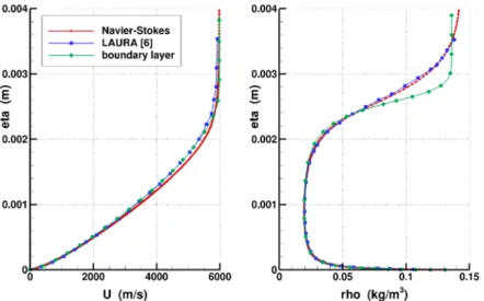
The steady mean flow past the cone was computed first for the five altitudes by solving the Navier-Stokes equations for an axisymmetric geometry, interpolating the gas properties in a Mollier diagram. The prescribed wall temperature is given in [5] for the last altitude 24 km and in [7] for 30 km. It was estimated for the other altitudes using a simplified reentry trajectory model. To ensure a fine description of the shock wave all along the cone, a very fine mesh was used with 303 cells along the wall and 600 cells along the normal. Grid convergence was checked by gradual increasing of the number of grid points along the normal, until the solution does no longer vary. The velocity and density profiles were also computed using a boundary-layer solver and compared with full Navier-Stokes solutions and with the profiles given in [5], computed with the NASA Navier-Stokes solver LAURA. A satisfactory agreement was obtained, as can be seen in Figure 1, where are plotted the velocity and density profiles at abscissa x = 2 m for the altitude Z = 24 km.
4. LOCAL AND PSE RESULTS
Local stability analysis and PSE solutions were carried out for each of the five selected altitudes. The detailed results will be presented for only 3 altitudes but the synthesis in section 4.4 will include all the computations. For this kind of high Mach number flow, the most unstable perturbations are streamwise waves of acoustic nature called “Mack’s second mode”, the first mode being the classical Tollmien-Schlichting wave observed in lower-speed flows [1]. Therefore only 2D waves will be computed here.
4.1. Altitude Z = 36 km
Figure 2 presents the stability results for the highest altitude. The amplification rates are plotted on the left and the N factors on the right. First, it must be underlined that the frequency band of the unstable waves is far higher than in subsonic flows. Frequencies from 100 kHz to 900 kHz are encountered here, requiring special measurement techniques like PCB in test facilities. Then, it can be observed that LST and PSE give close results. This can be explained by the fact
that on this low-angle cone, the streamwise evolution of the mean flow is very slow and thus the hypotheses of local theory are rather well verified for short wave-length perturbations.
The frequency of the unstable waves can be related to the boundary-layer thickness. Thus it is not surprising to observe a decrease of the peak frequency downstream, where the boundary-layer is thicker. At this altitude, the maximum value reached by the N factor is about 6 at 140 kHz, which seems insufficient to trigger the transition. Indeed the transition was not observed in flight at this altitude.
4.2. Altitude Z = 30 km
The N factors computed at altitude Z = 30 km are plotted in the left graph of Figure 3. In flight, the transition was observed at abscissa x = 2.9 m, corresponding to NT values
of 10 with the local approach and 9 with the PSE, both at frequency 270 kHz. A value NT = 7.9 at 240 kHz is reported
by Malik [7] for local stability and 9.8 for PSE, both with chemical equilibrium gas, as in the present work. PSE solution is thus seen to be less unstable than LST in the present work, whereas it was the opposite in [7]. However, the stability analysis depends strongly on the quality of the mean flow computation and thus some small differences on the mean flow can induce some deviations of the stability results. A value NT = 8.7 at 250 kHz is reported by Johnson
& Candler [8] for PSE with a nonequilibrium gas, computed on a refined grid with 400 cells along the normal.
4.3. Altitude Z = 24 km
The right graph of Figure 3 shows the N factors computed at the lowest altitude Z = 24 km. As pointed out by Johnson & Candler [9], below 30 km the transition abscissa measured in flight was different between both sides of the cone. This may be due to a wrong angle of attack or to a body deformation caused by differential heating. So both transition locations, denoted xT1 and xT2 in Figure 3, are
taken into account. Due to the higher Reynolds number, the boundary layer is now far thinner than in the previous cases and the frequencies of the unstable waves now reach 800 kHz. The critical N factor lies between 13 and 16 for local stability and between 10 and 14 for the PSE.
Attention should be paid to the eigenfunctions. Some examples are plotted in the next two figures, taken at the same abscissa x = 1 m. At 500 kHz, the eigenfunctions plotted in Figure 4 exhibit an exponential decrease outside of the boundary layer. On the other hand, at the higher frequency 900 kHz, the eigenfunctions plotted in Figure 5 exhibit a fast oscillation with slowly decreasing amplitude. This induces a strong constraint on the mesh in the normal direction for the stability computations.
4.4. Synthesis
All the stability computations are summarized in the last two pictures. Figure 6 shows the value of the N factor at the transition abscissa on both sides of the cone, computed with LST and PSE. It appears that this value varies more or less regularly, depending on the considered side. On the upper side, the PSE give a value close to 10. These results can be compared with those of Johnson & Candler [9], for a thermochemical nonequilibrium gas mixture. They obtain a similar result for the upper side but surprisingly they obtain lower values on the lower side. However they point out the key influence of the nose radius, whose estimation in flight may be somewhat inaccurate.
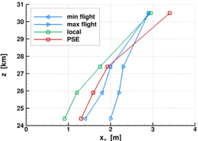
Changing the point of view, the last Figure 7 shows the transition abscissa estimated with LST and PSE, taking a constant value NT = 10. This abscissa is compared to the
transition location measured in flight on both sides of the body. Both stability approaches predict rather well the advance of the transition towards the nose when the altitude decreases. In the present case, slightly better results are obtained with the PSE.
5. CONCLUSION
The ability of two linear stability analysis methods to estimate the position of the laminar-turbulent transition has been tested on the trajectory of the Reentry-F flight test. Local stability equations and parabolized stability equations have been solved for five points of the trajectory. The high-enthalpy air was modeled by chemical equilibrium gas mixture. Relying upon the well-known eN method, both methods predict an advance of the transition location when the altitude decreases and the Reynolds number increases, for a constant Mach number. However, the uncertainties on some experimental parameters such as the nose radius or the effective angle of attack induce a range of uncertainty of the
N factor value at the transition.
Taking a constant value for NT all along the trajectory is
not necessarily justified since the free-stream turbulence level could vary with the altitude. However, doing so allows having a first approximation of the transition location. The PSE solution seems to give slightly better results, in accordance with the fact that they include higher order effects than the strictly local stability theory. Further computations should be carried out on different flight tests to refine the transition prediction method based on linear stability analysis of the boundary layer. In particular, the cross-flow instability appearing for a non null angle of attack should be carefully investigated.
ACKNOWLEDGEMENTS
This work was partially funded by a grant from the French Commissariat à l’Énergie Atomique et aux Énergies Alternatives (CEA).
REFERENCES
[1] L.M. Mack, “Boundary-Layer Linear Stability Theory”,
Special Course on Stability and Transition of Laminar Flows,
AGARD Report No. 709, 1984.
[2] T. Herbert, ‘Parabolized stability equations”, Annual Review of
Fluid Mechanics, Vol. 29, pp. 245-283, 1997.
[3] P. Stainback and C. Johnson and L. Boney and K. Wicker, A
comparison of theoretical predictions and heat-transfer measurements for a flight experiment at Mach 20 (Reentry F),
NASA Technical Report TM X-2560, 1972.
[4] C. Johnson, P. Stainback, K. Wicker and L. Boney,
Boundary-layer edge conditions and transition Reynolds number data for a flight test at Mach 20 (Reentry F), NASA Technical Report TM
X-2584, 1972.
[5] W. Wood, C. Riley and F. Cheatwood, Reentry-F flowfield
solutions at 80,000 ft, NASA Technical Report TM-112856, 1997.
[6] M. Malik, T. Zang and D. Bushnell, “Boundary layer transition in hypersonic flows”, AIAA Paper 90-5232, AIAA Second
International Aerospace Planes Conference, Orlando, 1990.
[7] M. Malik, “Hypersonic flight transition data analysis using parabolized stability equations with chemistry effects”, Journal of
Spacecraft and Rockets, Vol. 40 No 3, pp. 332-344, 2003.
[8] H.B. Johnson and G.V. Candler, “Hypersonic boundary layer stability analysis using PSE-Chem”, AIAA Paper 2005-5023, 35th
AIAA Fluid Dynamics Conference, Toronto, 2005.
[9] H.B. Johnson and G.V. Candler, “Analysis of laminar-turbulent transition in hypersonic flight using PSE-Chem”, AIAA Paper
2006-3057, 36th AIAA Fluid Dynamics Conference, San Francisco,
Figure 1: comparison of mean flow velocity and density profiles, Z = 24 km, x = 2 m
Figure 2: amplification rates (left) and N factors (right), Z = 36 km
Figure 4: eigenfunctions, Z = 24 km, x = 1 m, f = 500 kHz
Figure 6: N factor value at the flight transition abscissa (1: upper side, 2: lower side)