Diffusion models for computer-communications network

DIFFUSION MODELS FOR

COMPUTER-COMMUNICATIONS NETWORKS

by

Jose H. Barbera

This report is based on the unaltered thesis of Jose H. Barbera, submitted in partial fulfillment of the requirements for the degree of Master of Science at the Massachusetts Institute of Technology

in June, 1976. The research was conducted at the Decision and Control Sciences Group of the M.I.T. Electronic Systems Laboratory with partial support provided by the Advanced Research Project Agency of the Department of Defense under Contract N00014-75-C-1183.

Electronic Systems Laboratory

Department of Electrical Engineering and Computer Science Massachusetts Institute of Technology

methods derived earlier for message routing, can be used.

Finally, a comparison is made between the expressions obtained by dif-fusion techniques and those corresponding to the classical exponential M/M/1 queue.

by

Jose Heredia Barbera

Ingeniero de Telecomunicacion

E,T.S, IT,, Universidad Politscnica de Madrid (1971)

SUBMITTED IN PARTIAL FULFILLMENT OF THE REQUIREENTS FOR THE DEGREE OF

MASTER OF SCIENCE at the'

MASSACHUSETTS INSTITUTE OF TECHNOLOGY June, 1976

Signature of Author ... ,,...

Department of Electrical Engineering and Computer Science, May 7 1976

Certified by ,.,...., ,.,,., Su...iso.

Thesis Supervisor

Accepted by ,,,,,,,,, ,,,,,,*,,,.,,,,, .., ,, ,,,,,,.

Jose Heredia Barbera

Submitted to the Department of Electrical Engineering and Computer Science on May 7, 1976 in partial fulfillment of the requirements for the Degree of Master of Science.

ABSTRACT

The diffusion theory is used to model a computer-communication network in which messages flow from one computer center to another. The idea is to approximate the various queueing processes that occur in the system (of discrete nature themselves) as continuous-state processes. The messages waiting at the queues to be transmitted are considered of small duration so that in the limit the flow of messages is continuous.

With these ideas a general model for routing of messages in a computer network is established and expressions for the diffusion

parameters (drift and covariance per unit time) are derived in terms

of the network traffic. The mean length of the queues can thus be calculated and procedures to minimize the system overall queue size may be applied.

Examples for simple networks are shown. One of them corresponds to a load-sharing computer system and it is indicated how the general diffusion methods derived earlier for missage routing, can be used.

Finally, a comparison is made between the expressions obtained by diffusion techniques and those corresponding to the classical exponential M/M/1 queue.

THESIS SUPERVISOR: Adrian Segall

TITLE: Assistant Professor of Electrical Engineering and Computer Science

of this thesis.

This work was supported by the Fundacion del Instituto Tecnologico de Postgraduados of Spain and by the Advanced Research Project Agency of the Department of Defense (monitored by ONR) under Contract number N00014-75-C4183.

Acknowledgements III

TABLE OF CONTENTS IV

LIST OF FIGURES VI

1.- INTRODUCTION 1

1.1,- General Considerations 1

1.2.- Existing Models for Networks of Queues 4

1.3.- Objetives of this thesis 7

2.- THE DIFFUSION PROCESS 9

2.1.- The random walk process 9

2.2,- The diffusion process as a limit of a random walk 11

3.- SOLUTION OF THE DIFFUSION EQUATION 15

4.- DIFFUSION MODEL FOR MESSAGE ROUTING IN A COMPUTER NETWORK 18

4.1.- The general model 18

4.2.- Diffusion approximation for the routing model 23 4,3.- Calculation of the diffusion parameters 26 4.4.- Conditions for the diffusion to be valid 36

4.5.- Optimization procedure 38

5.- ILLUSTRATIVE EXAMPLES 44

5.1.- Example with two queues 44

5.2.- Example with four queues 70

5.3.- Diffusion approximation for computer load sharing 85

6.- COMPARISON BETWEEN THE DIFFUSION MODEL AND THE M/M/1 112

6.1.- Single queue 112

7,- CONCLUSIONS AND SUGGESTIONS FOR FURTIER WORK 124

REFERENCES 127

LIST OF FIGURES

Fig. NO. Title Page NO.

2,1. A random walk 10

2.2. Diffusion process as a limit of a random

walk 11

4.1. General configuration of a

computer-communication network 20

4.2. Detail of the queueing process at one node 22 4.3. Steady-State p.d.f. of a diffusion process 25 4.4. Average length of a diffusion queue in

Steady-State 27

4.5. Arrival and departure processes in a queue 28 4.6. Arrival and departure processes involved

in two queues 31

4,7. Detail of all queueing processes in a

network of four nodes 34

5.1. Network of three nodes: two sources and

one destination 45

5.2. Network of three nodes. Queues detail 46 5.3. Example 5.1. Routing variables and Fmin

in terms of q₁₃ 53

5.4. Example 5.1. Routing variables and F in

in terms of q₂₃ 54

55.5 Example 5.1. Routing variables and Fi _n

in terms of q₁₂ 56

5.6. Example 5.1. Routing variables and F

in terms of q₂₁ min 57

5.7.- Example 5.1. Routing variables and Fi

in terms of p₁₃ 58

5.8 Example 5.1. Routing variables and Frin

Fig. NO. Title Page NO

5.8a. Variation of the first derivative of the average

queue length in terms of ~ 61

5.9 Example 5.1. Routing variables and F in terms

of q9 rin 64

q

13

5.10 Example 5.1. Routing variables and F in terms

of q_{2 3} 655in

5.11 Example 5.1. Routing variables and Frin in terms

of q_{1 2} 66

5.12 Example 5.1. Routing variables and F . in terms

of q₂₁ 67

5.13 Example 5.1 Routing variables and F in terms

of p13 min 68

5.14. Example 5.1. Routing variables and F in terms

of P23 min 69

5.15. Network of three nodes, 3 sources and 2 destinations 70

5.16. Network of three nodes. Detail of queues at each

node 71

5.17. Example 5.2. Routing variables and F in terms

of q₁₂ in 78

5.18. Example 5.2. Routing variables and Fm in in terms

of q2₂₁ 79

5.19. Example 5.2. Routing variables and F i_n in terms

of q_{3 1} mn 80

5.20, Example 5.2. Routing variables and F in terms

of q₃₂ min 81

5.21. Example 5.2. Routing variables and F.. in terms

of q min 82

13

5.22. Example 5.2. Routing variables and F . in terms

of q2 3 min 83

5.23. Example 5.2. Routing variables and F in terms

Fig. NO, Title Page NO.

5.24. Example 5.2. Routing variables and F in terms

of p₂₁ in 86

5.25. Example 5.2. Routing variables and F in terms

of P₃₁ 87

5.26. Example 5,2. Routing variables and Fmin in terms

of p3 2 88

32

5.27. Load sharing example between two computers 90 5.28, Equivalent representation of the load sharing

example of figure 5.27. 93

5.29. Example 5,3. Control variables and F . in terms

of q13 101

5.30. Example 5.3. Control variables and F in terms

of q min 102

31

5.31. Example 5.3. Control variables and Fmin in terms

of p1 2 103

5.32. Example 5.3. Control variables and F in terms

of p34 min 104

5.33. Example 5.3. Control variables and Fmin in terms

od q - 106

13

5.34. Example 5.3. Control variables and F in terms

of q₃₁ min 109

5.35. Example 5.3. Control variables and F in terms

of p₃₄ 110

5.36. Example 5.3. Control variables and F . in terms

of p 111

12

6,1, Average length of a diffusion queue (solid lines)

and an exponential M/M/1 queue (dashed lines) with

the same drift for different size of buffer N 115 6.2. Network of three nodes and two queues 117 6.3. Variation of z* in terms of 61 for minimum

average queue length in example 5.1. 121 6,4. Comparison between the diffusion model results

(solid lines) and the M/M/l model (dashed lines)

1.1.- General considerations

A computer-communication system consists of several computers interconnected by communication channels. It is usually referred as a network in which the nodes represent the computers and the links represent the interconnecting channels, Messages are originated at some node and

have to reach some other destination node according to some routing strategy which will try to use the network in an efficient way.

The computer network considered here is assumed to operate in the "store and forward" mode: a message generated at a computer center will be directed into the appropiate outgoing channel according to the routing

policy and will be transmitted over this channel if it is free for transmission. If the channel is busy, the message will be stored at the node in some buffer joining other possible waiting messages. When the channel becomes free one of the wating messages is transmitted through the channel according to some queueing priority basis. This will be assumed "first-come, first-served" (FCFS) as it is usually referred in queueing literature. [7, 12, 22]

The queue of messages at each node- constitutes a queueing process

of discrete nature ni(t) such that ni(t) = Ai(t) - Di(t) where Ai(t) and Di(t) represent respectively the arrival and departure processes at node i, namely the number of arrivals and departures at the queue i up to the

In order to provide mathematical tractability a model for the network of queues has to be established.

The type of queue depends on the statistics of the interarrival and service times. The simplest type of queues is the M/M/1 queue (*). This means that the interarrival and service times are independent and obey an exponential distribution or equivalently- that the arrival and service rates follow a Poisson distribution, Because of the Poisson property

(see [17] for example) the expressions of the system dynamics are easy to obtain and the steady-state distribution of the queue length Pn is quite straightforward [7] :

pn-

(1-

) "n n = 0,

1,

2, .. (-la)

f

>>/}U

- c 1 (l-lb)

where

X

andi are respectively the arrival and service constant rates expressed in messages/unit time.

The condition XC is necessary to assure that the steady-state is reached and the process does not blow up.

The expression (1-1) allows to calculate the average queue length

(*) In queue literature it is usual to denominate a queue by the

symbols A/B/X/Y/Z where A indicates the interarrival-time distribution B the service-time distribution, X the number of parallel: servers Y the restriction on the queue length capacity and Z the queue discipline. Often the last two symbols are omitted and it is understood that Y = oo, that is no restrictions on the maximun queue length and Z = FCFS ("first come first served"),

The symbols used for A and B are: D for deterministic, M for

exponential, Ek for erlagian type k, G for general and GI for general independent. (Reference [7] )

n = n Pn' From the same expression, the waiting time distribution

(including also the time spent in the service, ie, transmission through

the channel) can be obtained and from this the average waiting time can

be drawn, An alternate way is using Little's formula [15] which states

that the average number of customers in a queueing system is equal to the

average arrival rate of customers to that system, times the average time

spent in the system:

n= E T] (1-2)

so that E [ T] can be calculated yielding

ET] = 1 (1-3)

In the computer network Ei T] is the average delay a message suffers going from one node to another and includes the average waiting time at

the entering node plus the average transmission time in the channel.

When a network of queues is considered, the messages arriving at a

new node along their path lose the independence property mentioned above

because of the strong dependency between interarrival times and lengths of

adjacents messages. For example if a message at node i has a length of s1

seconds and arrives at node j at time tl, it is clear that during the interval (tl, tl, + sl) no messages can arrive at j from i since they are transmitted in a sequential order, and therefore the independence assumption

is no longer valid. This makes the analysis very complicated from a

mathematical point of view, Kleinrock [11] overcomes this difficulty by

introducing the "independence assumpption" which specifies that each time

(exponentially distributed),

With this assumption an expression for the average delay over the entire network can be found in terms of the average delay in each link.

The desired routing strategy is that which minimizes the average delay and procedures to obtain the optimal strategy have been derived for example in [1] .

1.2.- Existing Models for Networks of Queues

One of the earliest models was established by Jackson 8 . He

considered an arbitrary network of N nodes each of them consisting of

ri servers with constant exponential mean service time ji. Messages

arrive at each node i from outside the network according to an homogeneous

Poisson process of rate X,. Each message upon being served, is directed

to some other node j according to some probability

eij

or leaves the

system with probability 1-

e.

ij. The transition probabilities

eij

are assumed corresponding to a 1st order Markov chain. The total arrival rate at each node i qi consists of the sum of the arrival rate from outside the network (Poisson) and the arrival rates from other nodes within the network:

i= i+ l

rj

ei (1-4)

3=1

Jackson showed that when i < ri _i for all i as far as the steady

state is concerned, the network behaves as if all nodes were independent Poisson processes M/M/ri with rate

Fi.

Therefore the steady-state joint

distribution can be expressed as the product of the corresponding marginal distributions, and expressions for the queue lengths and average delays can be easily found.

In a subsequent work [9] Jackson considered a more general network in which the arrival process still being Poisson, is allowed to have a rate dependent on the total number of customers in the network. Each node has r_i servers and the service time is exponentially distributed with mean dependent on the number of customers at that node. Still the joint

distribution factors into the product of the marginal ones and each node can be treated independently.

A modification of the Jackson's model was considered by Gordon and Newell [6] . They consider a closed system of queues which handles a finite and fixed number of customers. This model can be made equivalent

N

to that of Jackson by assuming i O0 for all i and E ij = 1. j=l

More general models that allow a service time discipline not

necesarily exponential, have been considered and explicit solutions have

been obtained, 120] .

In all cases the main difficulty comes from the fact that there is a very large system of equations due to the enormous number of states.

In order to overcome these difficulties and break away from the sometimes too simplistic models that assume exponential service time,

different approaches to network analysis have been made. Thus for example

Kingman [101 has shown in his treatement of heavy traffic theory that

properties of nearly saturated queues are rather insensitive to the specific form of arrival or service distribution.

The heavy traffic approximation is based upon the central limit

theorem. This leads to the idea of approximating a discrete-state processes by continuous-state ones which have been called diffusion processes and will be explained in a subsequent section.

The idea of approximating a discrete-state process by a diffusion

one is not new. (See for example Feller

[3]

). Nonetheless is rather

recent. Thus for example, Newell [16] gives an extensive treatement

of queues with time dependent arrival rate by using the diffusion

approximation. Gaver [4] applies diffusion approximation techniques to the waiting time in a M/G/1 queue. He shows that the waiting time is

exponential in the diffusion approximation provided the system was

initially empty. An asymptotic approximation is supplied for the mean waiting time near saturation and comparisons are made with the exact

solutions provided by the classical methods (see [7] for example). The

results show to be rather accurate for those conditions.

Gaver and Shedler [5] have applied the diffusion approximation

to evaluate the CPU utilization of a multiprogrammed system represented

by a cyclic queueing model. Solutions appear to be easier than the classical ones and yet the accuracy seems quite adequate; for the case studied₂

Kobayashi [13, 14] has analyzed a system of queues by diffusion

methods. His model is based on the Markovian model of Jackson (open networks) and Gordon and Newell (closed networks) which we mentioned earlier. In the first paper [131 and based upon central limit theorem arguments he finds the steady-state distribution of a single queue, and a system of queues (open and closed) assuming independent identically distributed interarrival

and service times with general distributions. In the second paper [14] and using diffusions methods too, the transient behavior of those systems

is analyzed. The analysis provides an estimation of the transient period which shows to be shorter as the system is less congested. A comparison -of results with those exactly known by classical methods is given in [19]

and they show to be rather accurate for utilization factors near 1.

1.3.- Objetives of this thesis

As it was pointed out in the preceeding section when the number of states of a Markov model becomes very large, although finite, the search of solutions appears quite cumbersome. The procedure of approximating the discrete-state process by a diffusion process can be therefore useful

because mathematical methods associated with a continuous space are very often more easily treated than those in a discrete-state space. In a

computer-communication network this is the case when the number of computer centers is relatively large.

The purpose of this thesis is to consider a general type of computer network and by using diffusion methods find a model for analysis of the behavior of the network. Then a strategy for routing messages throughout the system in an efficient way is to be found. In order to make an optimal use of the network, messages shall reach their destination as soon as possible and thus the performance criteria for routing will be to minimize the overall

average delay on the entire network.

of [23] assumes a deterministic scheme with known traffic-inputs whereas

here the model is stochastic in the sense that the inputs are-only known

2.- THE DIFFUSION PROCESS

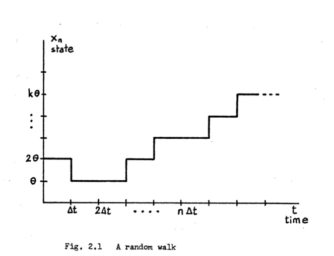
2.1.- The random walk process [21

It is introduced here the concept of random walk as a discrete-state discrete-time Markov process for the diffusion process can be drawn from

it in the limit. Consider the time divided in intervals of duration

At

:

0,

At, 2 At, ... n t ... and the state divided in intervals of

length

e

: 0, , 2e , ... ke ... . At time t = 0 the state is x 0= k

e.

At time t = At the state can jump one step

0

upwards with probability p, one step downwards with probability q or remain the same with probability 1 - p - q. No other transitions are allowed. In each interval of time later the same jumps with the same probabilities can happen and are

independent of the previous jumps. This is graphically shown in Fig.2.1 and can be considered as the motion of a particle in a one-dimensional space. If the particle continues to move indefinitely the random-walk is said to be unrestricted. Nonetheless it is frequently necessary to have the motion restricted in some way, usually by the presence of "barriers". For example a random walk starting at the origin can be

restricted to move between an upper barrier a > 0 and a lower barrier at b < O. Several types of barriers are encountered, One of these is an

"absorbing barrier": when it is reached the particle stays there and the motion ceases. Another type is a "reflecting barrier" defined as a state that when crossed in a given direction, say downwards, holds the particle

staeI

ke.

2 L

At

2At

.

n

At

t

time

Fig. 2.1 A random walk

until a positive jump occurs and brings the particle out of the barrier resuming the motion,

We shall examine here the properties of a random walk with reflecting barriers, It is of interest to determine the steady-state or equilibrium

distribution of the state as t goes to infinity.

Clearly the dynamics of the random walk _{exposed above are governed}

by the following equation:

Pk (n At + At)

pke

_{(n At) (l - p - q) + P(k-1) (n At) p}

₊

+ P(k-l)e (n At) q _{(2- l)}

where

Po (n At)

f

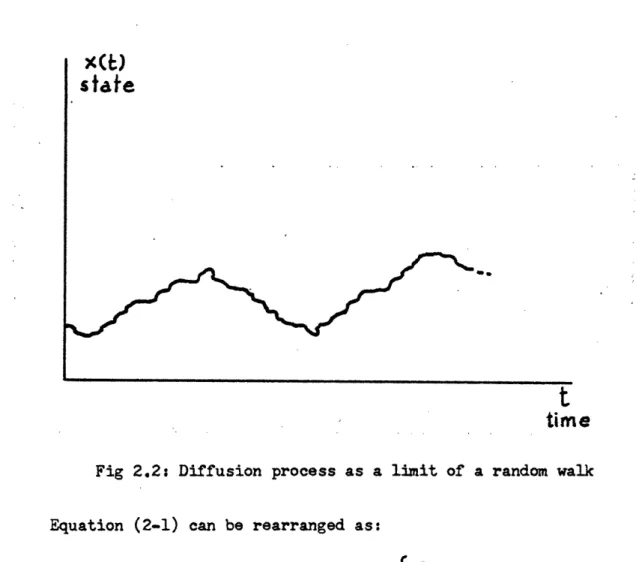
Prob. of being at state = ke at time nAt given that thel

Consider the random walk of section 2.1. Assume that

0

and At go

to zero so that n At - t and kI -~ x(t). The resultant process x(t)

becomes a continuous-sate continuous-time- Markov process. It is shown in Fig. 2.2

state

time

Fig 2.2: Diffusion process as a limit of a random walk

Equation (2-1) can be rearranged as:

P

(n At+ t) Pk(n At)= *

4

{

[P(k+l)(nAt) - Pico(nAt)J ]

-

[kIe

(nAt)

-

P(k-l)Q

(in

At)]

+

2

P(k+l){

(n

At)

mce(n At)]

+

[Pke

(nt)-

P(l)

(nAt)]

(2-2)

When 6t becomes very small, so that n t-- t, kG --_ x(t) and ko

-

x0o

the state probability: Pke (n

At)

-- p(x;t/xo).

Let At = K 2 (K being a constant) and divide both sides of (2-2) by At. Then

p(x;t + At/xo) - p(x;t/xo)

At

p+ q 1 [ p(x+e;t/xo) - p(x;t/xo) p(x;t/x_o ) - p(x- 8;txo)

2K

e

"

e

p - q 1 p(x e;t/xo) - p(x;t/xo) p(x;t/xo) - p(x- e t/xo)

2K

[px* etx

-

(

t/o

Taking limits when At- O

e0

-

o

bp(x;t/xo)

=li

p

+

1

[1p(x;t/x

O

)

bp(x-e ;t/xo)

at

.

e-o

2K

.L

x

.x

(2-4) -Pi - q 1 bp(x;t/xo)

6p(x-

;:t/x O) _ 1, x +2 _ bx if in O p +q K= (2-4a) and Jim (2-4b) Mo Ke =

oC and A being constants then (2-3) becomes

p(xt/x) P(xt/Xo) p(x;t/Xo)

bp t

₁

0x(/x -: -. x (2-5)

which is the diffusion equation [2 ].

For the conditions (2-4) to be satisfied, the probabilities p and q must be taken as:

p

=

K

(. +

= 2 ( +

')

(2-6)

1 K la

q = K : (OC e- ) =2 ( t (2-7)

that is the probabilities of jumping upwards and downwards have to be nearly the same, the difference being a term that tends to zero as it.

Notice that the parameters 3 and cM are respectively the incremental mean and variance of the process x(t) per unit time since

E [x(t + At) -x(t)/x(t)] =

.(p

- q) - (Ke2) =-.At

Var [x(t + At) - x(t)/x(t)]= 2(p + q) -

e

2(p - q)2

--b

e

2

K(of_

,

2

92)

=

c.

At

that is

13

= im E [x(t +

At)

- x(t)/x(t)] m E [x(t)/x(t] (2-8)

AtO-0

At

At-O

At

io = li. Var [x(t+

At)-x(t)/x(t))]

im a (2-9)

At-0

At

-

=

O-0

At

t

In general the parameters om and P can be dependent on the state x(t). We can consider as well a multidimensional diffusion process x(t) with vector mean per unit time 2 and covariance matrix per.ui.it:time

A

=

[ij]

.

In this case the diffusion equation relates the derivatives of the multidimensional p.d.f.p(x;t/x₀) and the expression (2-7) becomes

bp(X;t/xo) 1_ _ _2p(X;t/xo) e. p(x;t/Xo )

...bt = i= l 2 «it 8'- i bxj tX (2-10)

wheri=e j=1isth n oxi j i=l

E[Axi(t)/ x(t)]

1/~~~3i-~ at(2-11 limo

At- O

At

Cov

[x i(t) Ax.(t)/ x(t)]

04is t-O~~~~ lJ - (2-12)

At

i = 1, 2, ... m

The probability of each process i (i = 1,2,... m) jumping upwards Pi

and downwards qi have to satisfy now the conditions (2-6) and (2-7) for each process xi(t) to be considered as diffusion, and similarly for each

individual process it must be At = Ki

e.2

where the constant Ki are in

principle different,

In the computer-network system we are interested the state of each

process represents the total number of messages that are waiting to be transmitted at an specific queue. For each queue i there is a lower

reflecting barrier at xi = 0 because the number of messages in a queue

cannot be negative. If there is no restriction on the queue length, then there is no upper barrier. Practically the size of the queues are limited by the length of the buffers where the messages are stored. Therefore an

upper barrier is to be assumed too which if reached indicates that the buffer is full.

3.- SOLUTION OF THE DIFFUSION EQUATION

The solution of (2-5) or (2-10) depends upon the conditions imposed

on x(t). If x(t) is allowed to take any value: - 00 < x(t)< +oo the

joint p.d,f, (p(xQ;t/__O) solution of the diffusion equation is the corresponding to a multidimensional Wiener process with mean At and covariance matrix A

t:

ep[-

(x- ,- t)T (At)

1

(

-

-

t)]

(3-1

p(x_~; t/x~o) =

.

.

.

.

.

.

...

-- (3-1)

(2 n)m/2

J AtJ/2

.

(Taking in (3-1) the derivates a/ axi, ?2/ox_i 6 x and /

/t,

it can

be easily seen that (3-1) satisfies expression, (2-10).

Observe that (3-1) has no steady-state solution when't --Oo. If one reflecting barrier is considered, say at x = O, the solution

of the scalar diffusion equation (2-5) with initial condition p(x;O/x₀) =

6 (x - x) can be found by using the method of images [24]and it is [2]:

p(x ;t/xo) = t{e[t ) ] exp- exp .. 2 .. xO )

ex[ (x+ 3 t)2 + 2 I I exp - 2I ax

2 o Bt

/

where 22

4()=eu2/2 du

The first term of (3-2) corresponds to the transient period and the second one is the steady-state term. By inspection of (3-2) it is easy to see that when t -- C the first term of (3-2) vanishes and the second one becomes

0 p/>0

lim p(x; t/x_O) = p(X) = (3-3)

t -02~

exp

x

1,

-

;

3

<

O

f or x ? 0

that is an: steady-state solution exist for negative drift which physically means that the service process has to be faster than the arrival process so that the length of the queue does not become infinite,

If two barriers are considered at x = 0 and x = a > 0 for example then the equation (2-5) for the scalar diffusion with initial condition p(x; O/x_o) = 6(x - xO) and boundaries O x(t) < a,can be solved by the separation of variables method and the solution is: [25]

exp

a....

+

. 82 . exp (x x)

p(x;t/xO) 2ps x4- 2x) + eXpI t exp

(3-4) 00

4 exp ( 2 DC t) n2

a Exp

n

A()f Yn(x) Yn(xO)

n-n=l n2 _{+ ( )}2

and = n ; n =O,± , +2

Yn(x) = cos XnX + . sin XnX

Regardless of the sign ofS there is a steady-state solution when t - 00.

This distribution denoted by

p(x) = lim p(x; t/xo)

t

-00

can be obtained by taking limits in (3-4)

2 exp |$ x

)

p(x) _xp Oax a ; (3-5)

For the multidimensional process, define a vector

jX

-.

2

g2A

_(3-6)

and then the steady-state distribution of the process x(t) can be obtained by equating to zero the right hand side of (2-10).

This gives [14] m p(x) - lin P(x; 0o) Pt/xPi(xi) (3-? ) t - 00 i=l where

6

iX Pi(X) = i ; O SXi ai (3-7b)

4.- DIFFUSION MODEL, FOR MESSAGE ROUTING IN A COMPUTER NETWORK

4.1.- The general Model

Let us consider a general network of N computer centers (nodes).

The same notation as in [23] will be followed. Each node can be connected to any of the remaining (N-I) nodes in both directions. We have then a possible total number of communication lines N(N-1).

The nodes will be represented by letters i (i=1,2, ...,N) and the

branches by pairs (i,j) (i,j = 1,2, ... N I i i j). Call

I(i) the set of branches entering node i

D(i) the set of branches coming out from node i

At each node there can be a maximun of (N-l) queues where messages

with destination any of the other remaining nodes wait to be transmitted.

Clearly the total number of queues in the whole system M is such that

M SN(N-1). I

The queueing processes are of discrete nature themselves as was

pointed out in a preceding section. The diffusion model that is stablished

here makes the approximation of considering them as continuous processes.

In order to do this, the messages (that in principle have different lengths) are assumed to be divided in small packets of duration At units of time.

The time will be assumed divided in intervals (t, t +At) small enough so that the following events will occurs

aij(t) = Prob, that a message of length At with final destination node j arrives at node i from outside the network.

1 - aij(t) = Prob that no message of length at with final destination j arrives at node i from outside the network

i,j = 1, 2, .. N , i j j

Therefore during (t, t + At) only these former events can occur. The probability that more than one message comes is zero.

uki(t) = Prob. that a message of length At with final destination k is transmitted from node i to node j.

1 - uij(t) = Prob. that no message of length At with final destination k is transmitted from node i to node j

i,j = 1,2, ... N i 3

cij = Prob. that no message of length t is transmitted succesfully from node i to node j.

i,j = 1,2, ... N

:

i j

Observe that cij corresponds to the capacity of the link (i,j)

expressed in terms of probabilities rather than in traffic units.

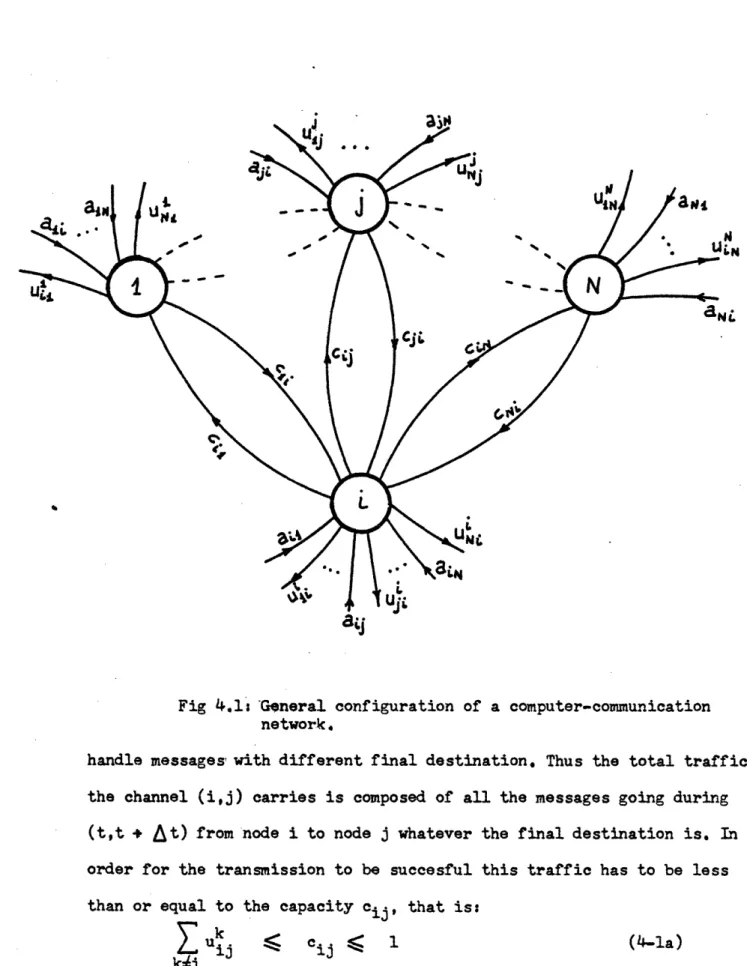
In Fig 4.1 a diagram of such a general network is depicted.

The capacities cij are fixed for each channel (i,j). The incoming

traffic probabilities aij(t) are quantities that depend on the amount of

users' demand at the specific time t. We shall consider this demand rate

to be stationary so that it will not be dependent on time but a constant

aij.

The outcoming traffic probabilities uij(t) are the quantities we

want to find according to the input traffic and the network fixed capacities so that the system performance is satisfied, according to some criteria as we shall see later. For the same reason as aij(t), the probabilities

k_{. (t) will be independent of time.}

N,,

Ij"' alit

Cj.

L~

Fig 4.1: General configuration of a computer-communication network.

handle messages with different final destination. Thus the total traffic the channel (i,j) carries is composed of all the messages going during (t,t + At) from node i to node j whatever the final destination is. In

order for the transmission to be succesful this traffic has to be less

than or equal to the capacity cij, that is:

and clearly ukj (i,) ( b)

The constraint (4-la) is necessary to have an errorless transmission. Now consider the queueing process representing the number of messages nij(t) that are waiting at node i to be transmitted to node j at the time

t. If finite capacities are assumed for the buffers, that is Nij is the maximun number of messages that can be stored at i to be transmitted to j,

then the ratio

xij(t) nij(t) (4-2)

Nij

represents the normalized queueing process so that

0 < xij(t) 1 i,j = 1,2, .. N i j

(4-3)

When the- message lengths At become very small it is clear that

xij(t), representing the amount of messages filling the buffer with respect to its total capacity, becomes of continuous nature and can be approximated by a diffusion process with two reflecting barriers at x = 0 and x = 1 as indicated in (4-3). The lower barrier represents the queue completely empty and the upper one representing the queue full.

At each node we can have at most N - 1 queues and in the whole system

the maximun number of queues is N(N-1). This can be visualized in Fig 4.2 for N = 3 in which node 1 has been magnified to indicate all the queueing processes that take place.

The switch S12 represents that the channel c12 can handle messages

from x1 2(t) with probability u2 and messages from x13(t) with probability

U₁₂ such that u2 + u₁₂3 c12'

a 1

Cis

1 with probability u₂₁ entering queue x13(t) and waiting to be transmitted to its final destination node 3.

4,2w- Diffusion approximation for the routing model

We saw in section 3 the steady-state solution of the M-dimensional diffusion equation (2-12).

The case we are dealing with is M . N(N-1) and the barriers for all

queues are 0 and 1.

The joint p.d.f. of the system is given by (3-7) with ai = 1 for

all i.

It was established in section 1.3 that the performance criteria

will be to minimize the overall delay messages experience (on the average) when they are transmitted from their origin to their final destination.

An equivalent condition is to minimize the average queue size of the whole system. To see this, consider one queue nij(t). If we call Aij(t) the number of arrivals at node i with destination j during (O,t) and Dij(t) the number of departures from this queue in (O,t) then

nij(t) = Aij(t) - Dij(t) (4-3)

represents the total number of messages waiting at that queue at time t. The quantity

t

0J nij( t ) dt (4-4)

is the total time all messages have spent in that queue during (O,t). The average delay per message at that queue will be:

E [Tiji =

I

nJ° M (4t5) Aij(t)

and the average number of messages waiting at the queue:

ft

E [nij(t)] j (4-6)

t

Therefore from (4-5) and (4-6) we see that minimizing the average delay is equivalent to minimizing the average queue length or normalizing acording to (4-2), minimizing E [xij(t)] .

In the discussion of section 3 about the diffusion process we

implicitely assumed that there were no idle periods, that is when the process reaches the lower barrier it does not stay on there but jumps up. This has not to be the case in general because with some probability

there will be certain idle periods in which the queue will be empty. This

probability of idle periods can be expressed in terms of the utilization

factor [12] which is defined as the ratio of the rate at which the jobs enter the system to the maximun rate (capacity) at which the system can perform this work. Calling this factor (<1) the probability of idle period will be 1 -P.

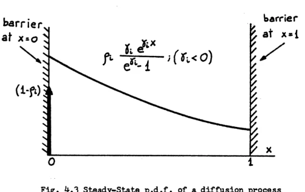
Therefore the p.d,f. (3-7b) shoud be modified to include the effect of idle periods and this can be taken into account by splitting

the p.d.f. into two parts. One representing the probability of empty

queue (an impulse of weight l-p) and the other representing the continuous distribution when the queue is not empty

pi(x) -fJi) J(x) + i -i O< x 1 (4.7)

~"`-~~~~~~-~~~"~'~~~~-~~II^`~~~~~~~---which is represented in Fig 4.3,

barrier

arrier

at x-o

at X

~~~~O -1.~~ X

Fig. 4.3 Steady-State p.d.f. of a diffusion process

The expected queue length for the i-th queue is calculated from (4-7)

1

E(xi)

=

xipi(x)dxi1

)

i

(48)

In Fig. 4,.3 the expression (4-8) is represented. As it ca be seen

O <E(xi) ( Pi' In the same figure it is represented the function

- 1/ ( ~i < 0i O) which would be the mean value in the case of no upper

barrier. We can see that for values of Xi less than -3 both curves

the queue length from increasing without limit and therefore it does not

become unbounded at = 0..i

The significance of the parameters ~i can be seen from Fig. 4.4:

Xi< 0 means the queue is on the average less than 0.5

Pi

full and >i 0 more than 0,5 full.

The overall mean value is given by

F( ff ) = t Pi ati, 1 (4i9)

and this is to be minimized over some region of the M-space determined from the constraints of the problem as we shall see in section 4.5.

4.3.- Calculation of the diffusion parameters

We want to find the components of the vector mean per unit time /

and the elements of the covariance matrix per unit time

A

defined in

section 2 (Eqs. (2-11) and (2-12)).

Consistent with the notation in section 4.1 let us redefine A and

A

as:

fli= hm 1 E [xij(t + At) - x(t) x(t)] =

At-O at

(4-10)

lim E [Axi(t) x(t)]

0 Uc, .. 0 0, 4.' 111IFT ~ ~ ~ ~ ~ ~ ~ 60 LO ci fr be *14 I ~ i ~ f i I4

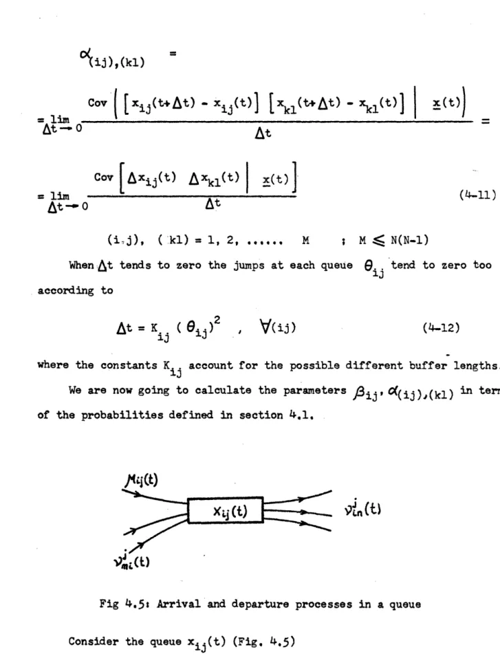
°(ij),(kl)

Cov

(

[xij(t+At)

ijt))]

[xkl(t+At) - ixkl(t)I x(t]

At 0 _At

Cov [Axi.(t)

Axkl(t)

I

x(t)]

E lim - (4-11)

At-.- 0

(ij), ( kl) = 1, 2, ... M s M N(N-1)

When At tends to zero the jumps at each queue

eij

tend to zero too according to

w h t = K.j (ij) (ij) (4i12)

: J ij

where the constants Kij account for the possible different buffer lengths.

We are now going to calculate the parameters Bij' O((ij),(kl) in terms of the probabilities defined in section 4.1.

Fig 4.5 Arrival and departure processes in a queue

Fig 4.5C Arrival and departure processes in a queue Consider the queue xij(t) (Fig. 4,5)

mE I(i) nED(i)

3 3

where for all t, ij(t), 9i(t),

))4t)

are Bernoulli independent random

variables that can take the following values:

ti.(t) =

e

with probability ai 44)

1J j ij

(4-14)

= 0 with probability (1 - aij)

3JJ (t) = with probability ui

mi = ~ij

= 0 with probability (1 - umi)

i3 (t) =

eij

with probability u (46)

(4-16)

= 0 with probability (1 - un)

according to what was established in section 4.1

Calculation of the incremental mean coefficients

The mean value of xij (t) is from (4-14) - (4-16)

E[Axi3 (t) x(t) = E [Axi(t) _

= ij aij* uj n (4-17)

m

(

I(i) mi nED(i) i n

Substituting ij = K and taking limits in (2-13) when

At - O, we obtain

/3i. = l~imE [6xi.(t)]

i A t -0 .Atdt (4-18) aj +)ui - ji Uin

13

lima m

j

At -O0 1/2 Kij t

for all pairs (ij) = 1,2, ... M ; M ~ N(N-1)

Calculation of the covariance matrix elements

--- Diagonal elements : from (4-13). since x .ij(t) is a sum of independent

random variables we have:

Var

[Axij(t)]

= Var [Jij(t) ] + Var [Ii(t)

]

+

mEI(i)

mfj

(4-19)

+

YI

Var

[ij

(t)]

nED(i) in

and substituting the value of the variance corresponding to a Bernoulli random variable we obtain:

Var Axij(t) = eij (jaij( ) + +Ui(l-ui) u *

m )

+ > u ( m-u j (4-20)

-- Off-diagonal elements: Consider two different queues xij (t) and xk.l(t) (Fig. 4.6)

zxijct)

_r/t(t)

x~i~t)

",k()

V;JW

Fig. 4.6: Arrival and departure processes involved in

two queues

i~j

m

j

pGI(k) e D(k ) q

Since )j (t) and $kl(t) are independent:

Coy [,ij(t)

4kl(t)]=

Coy [4Rij(t) )k(t)] = Cov [mi (tF)kl(t)]= 0

then

Cov xkl(t)1 C Vji~

V

j _{(t) 9 (t)}

-Co

[xij(t) Akl(t) mEI(i) pE I(k) mi pk

m j p fl

\\ j 1 \ \

q m Mi kq3t9mi kq(t) 3 -

L

n(t) pk(t)

nmDi) qDk) kqniD(i) pI(k)

+

DvqinW(t) tq() iiekl Umiupk

mC~~~~ j p 1

ne() qED(k) i kq n D(i p I(k) t ) p

j J j 1

neD(i) qED(k) _{. Uin . p}

1) m n I(i) p E I(k)

m j 1 p

j 1

Umiin Upk m,iqp, k

j

1

cannot be that; m,i = p,k and j = 1 )

(a) i(t) and pk are independent (queues at the same differnt nodes)

(b) Messages with different destination (j u 1) cannot go over the same

channel (m,i = p,k) at the same time t (see Fig 4.7, both queues are in the same node i = k)

(c) This case corresponds to the Var[9ji(t)] and was calculated

previously in (4-19). Observe that the terms corresponding to

(4-22a) when substracting the products of the means to obtain the covariance, will yield

V pk(t) -~t = pk

t

m(ti uk mi pk=

and the terms corresponding to (4-22b) will yield

y _mi (t) V (t) _{pk 3,,(t)} t) _3pm t) = 0 - Umi u_pk

2) m I(i) q D(k)

m.

j

ui u ; ,m,i k,q (a)

mi kq

V)i(tu 9 q(t) ' ; m,i = k,q and j ~ 1 (b) (4-23)

mi kq

u ; m,i = k,q and j =1 (c)

mi

The equations (4-23) are obtained because: (a) and (b) the same reason as in (4-22)

(c) it is the same random variable YJi(t) corresponding to two different queues xij(t) and xkl(t) which are in nodes i and k respectively. See for example Fig 4.7: Consider the processes x₁₂(t) and x32(t) belonging to nodes 1 and 3 respectively ( i=l, k=3, j=l=2)

4010~ ~~~~~~ .10lo~ ~~~~~~~ am 4%~~~~~~~~~~~~~~~~~~~4 4%~~~~~~~-,-

4~~~~~~LI~~~I~~~iE~~~&\

0~~~

,/ypŽt?

0

IT~~~~~~~~~~~~~~~~~~~ ~~~~~~~~~~1*~~~~~~~~~~~~~~... -w =% 'Z~~~ I cn~~~~~~~~~~~~c f;J~~~~~o 0 sj~~~~~~~~~~~~~~~~~~~~~~~~~~~~~~~~~~~~(

,

/ ~~ z -: 0c-I-I~I t0 r-·· ~H o to r4

x

I

I',

X~~~~~~

-i t-xl~~~~~~~~~~~~~~~~~~~r 1.1, _{0 0~~Zc} U 0 _{0~~~~~~~~~~~~~~~~~~~~~t} (I 0~~~ x"~~~~~~~~ -~~~~~~~~/ . w \ rz-- U, ! J. 4 3 \~~ 1 ~ ~~~~ I

-rx-L--'

4 IY S

S

r~~~~~~~~~

3) ~~~~~~~~~~~~~~~~~~~~C~~~_I~~ O~~~~~~~~4 -4%-

as indicated by (4-23c)

The term corresponding to (4-23c) in the covariance expression will be

35. (t)- u j Umi ) (1- (Umi) = ju

[9mi( )] [5)mi( ) ] mi ( mi) mi mi

3) nD(i) ; pE I(k)

This case is exactly like 2). Just interchange this subscripts i--k, m--p, q--n, j--l

4) nED(i) ; qED(k)

This case is similar to 1), The only difference is that it takes the processes coming out from node i and node k whereas in 1) we had the processes entering nodes i an k, Therefore the corresponding expression

is

Uin Ukq ; i,n k,q (a)

Wi

( ) 3 ( =) 0 ; i,n = k,q and j 1 (b)

cannot be that i,n = k,q and j = 1 (c) (4-24) According to this we can have several cases:

A) Both queues are in the same node i = k. In this case only the first and fourth term of (4-20) enter in the covariance (relating the inputs and outputs respectively):

Cov [Axijxii (Xil(t) =u - u Uin u

if~jg: mgj~jif n i

(N-3)terms (N-1) terms

(4-25) B) Both queues are m different nodes i $ k. In this case the 2nd. and

3rd. term of (4-20) appear. There are two possibilities:

B-I) Both queues have the same destination : j = 1

Co Xijt) Axkj(t) =- ui (1 - uik) - Uki (1 u ki)

ijkfj (4-26)

B-2) The queues have different destinations: j & 1

rA~[~x~j~t~ n~(t)] Aj I 1 I

Coy ₁[ ijx(t)

AXk

1(t)W = u uik ik Uki Uki

i~j kSl (4-27)

but observe that if k 4 j

Coy [FAx..t) Ax(t)] =WI uij ui. (because uji = 0)

ILAJi

j2.

ij uij 32

and if i = 1

Cov[ Axij A(t) i(t) = Uki i (because

ki uki (ecause Uik

4.4 Conditions for the diffusion to be valid

Going back to the expression (4-18), if Aij has to have a finite value it is necessary that the numerator of that expression tends to zero as (At) .

Recall what was established in section 2.2. concerning to the conditions for diffusion: for the variance and mean per unit time to

make sense the probabilitites of jumping upwards and downwards have to be "nearly" the same, the difference being a quantity depending on (At)1 /2 and therefore this difference decreases proportionally to

1/2

( t) when

At

tends to zero. This is reflected by the expressions (2-6) and (2-7).

Therefore let us assume that the probabilities aij and u.j are of the form of (2-6) and (2-7) that is a constant term plus another

depending on (At)l/2, that is:

aij = Aij (4-28)

U = Uk ./ At (4-29)

iij ijl ij +

The channel capacities which are related with the service process will be considered of the same form too, that is a fixed term plus another varying with ( At)1 /2 as shown:

Cij = Cij qij (4-30)

which means that the capacity of channel i - j is variable about a fixed value Ci in a quantity proportional to (At)l/2

Then the conditions that have to be satisfied for the diffusion property, are obtained by plugging (4-28), (4-29) and (4-30) in (4-18). Thus we obtain:

Ai3 + ) U

ii=O

(4-31)

m I ) mi neD(i) in

Pij + Yi ' =,6ij (4-32)

mI (i) n D(i) in Ki

m

j

for all pairs (i. j) = 1, 2, .,. M ; M N(N - l)

The constants Kij are given by the buffer size. From (4-12) we see that K ij( _{i j )}2 = Kkl( kl)2 but i = 1/Nij and thus Kij/Kkl =

= (Nij/Nkl)2.

The expression (4-3!) is related with the deterministic flow at each queue and simply states the balance that has to exist at each node between inputs and outputs if the traffic were deterministic, whereas (4-32) gives an idea of the infinitesimal variation during (t,t + A t)

since the drift -3ij indicates de tendency of queue (ij) to increase

or decrease per unit time. Moreover from the capacity constraints (4-1):

i k ij (4-33

qik k

i k Yij Yij O (4-34)

4.5.- Optimization procedure

In the model we have established, we have a network whose channels cij are given and have fixed capacities. The input traffics aij depend on the users' demand so that are considered as fixed quantities too. The question is to find the best routing strategies within the system

k

which are represented by the probabilities ui defined in section 4.1

k

subject to the capacity constraints (4-1). The quantities u will be

ij

called routing variables and will have to be chosen to minimize the average queue length in the system according to the given input' traffic and the fixed capacitites. This is an open-loop type control procedure.

Note(Fig 4.7) that the maximun number of routing variables we can have per queue is N - 1 so that in the whole system we can have at most

M(N - 1) control variables.

The expression of the covariance elements follow from the

expressions (4-20), (4-25), (4-26), (4-27) and (4-11), (4-28), (4-29). Thus we have

Variance elements (recall (4-20))

A.J(l-A.)

Z

u (l -+ m) + u U(l- )

Umi m( in n

C((2 mj)

~(j2 ~jij (4-35)

Covariance elements: a) i = k; i ~ j f 1 (recall(4-2 ))

mE(i) mi U + E D(i) in Uin

O((ij),(il) - m ; (4-36) Kij il b) i k j = 1 (recall (4-26)) U ik(l U ) + UJ(l - U ik ki ki (4-37) O~(ij),(kj) = -T(4-37) ~Kij fkj

c) i & k; j 1 (recall(4-27)) j i i j U U +U Ui 0ik ik ki ki (4-38) (ij),(kl) i j kl

(Remember special cases of (4-27) when k = j or i - 1)

Therefore the covariace per unit time is a M x M matrix

A

which

depends on the M possible inputs A.. assumed to be given and on the L

control variablea U.where L M(N 1) . We wite

A

=

A(Au)

13

where A and U are respectively M and L dimensional vectors. Notice than the L routing variables Uk may not be chosen

ij

independently, because they have to satisfy the system of equations (4-31) so that only L - M variables are independent, provided that they

satisfy the capacity constraints (4-33).

We want to minimize the overall mean (4-9) that is

min F( = min

fij

(4-39)

all queues i=l e ij - 1

I-where Wij are the elements of the vector

5

defined as

6

= 2A -The drift vector _3 can be expressed in terms of the inputs Pij and the control variables yJi(m

E

I(i); m n j) and yJ (nE D(i)). From

(4-32) and using matrix notation:

A8=p+ H y (4-40)

Y/n ii n E (i)

for all possible pairs (i j) and where H is a M x L matrix depending on the specific configuration of the system and whose elements can be only + 1 for incoming links, -1 for outgoing links and 0 when there is no conexion

Then we have:

-=2A

- 1

_p

_{+ 2A}

_{H y (4-41)}

Call for convenience

2 1 = d (dM-dim.- vector) (4-42) and 2A-1 H = D (M x L matrix) (443) then -d

=

+ D (4-44)

and the problem is to find

min F(d + D ) (4-45)

where u = U + y . The minimization (4-45) is to be carried over the vectors U and Z with the constraints (4-31) and (4-33) on the vector U and with the constraints (4-34) on the vector i.

The constraints the elements of U have to satisfy are those given by (4-33) (capacity constraints) and (4-31) (flow balance at

each queue). In general for given inputs Aij and capacities Cij, the vector U satisfying (4-31) and (4-33) will not be unique, and for different choices of U the covariance matrix

A

will be different and

so will be the minimum of (4-45). In order to simplify the minimization (4-45) it will be assumed in this thesis that

A

is fixed, that is we have chosen a vector U satisfying the requirements of (4-31) and

(4-33) which represents an equilibrium situation for the system and we shall be interested in how the system will behave for small

alterations about the equilibrium situation. In particular we shall

seek how the routing variables y. .will vary so that the overall ii

average queue length of the system is minimum.

With this asumption the vector d and the matrix D are constant

and the minimization problem can be stated as :

min F(d + D I) = min F₁(X) (4-46a) subject to:

i j k 1 qij Yij (4-46b)

The aim is then to find the optimum vector y* that satisfies the minimization (4-46).

Notice that the function we want to minimize es a sum of M

functions like the one shown in Fig 4.4 which is convex for

6ij.

0 the meaning of this being that the queue is loaded less than or equal to 0.5 i on the average. Therefore if for all queues

6ij

<0 then

the function F(_A) will be convex and will have a well defined minimum over the constrained region. The convexity property is convenient to

---include it when the minimum is searched by numerical methods starting

with some initial guess. Physically it reflects the fact that the messages

arriving at the nodes do not stack up at the queues so that the system behaves "nicely" and does not become congested.

5,- ILLUSTRATIVE EXAMPLES

Let us now apply the theory developped in the preceding sections to

some specific examples.

Our purpose is to minimize a function of L variables subject to some

constraints over a convex region.

Because of the exponential nature of the function (4-8) even with a

small number of variables it is not possible to find analytic solutions

and one therefore has to use numerical procedures.

The minimization procedure that will be used is based upon the method

of Zangwill [27] whichis a modification of Powell' s algorithm [18]

Basically an initial point and a set of L directions are chosen.

Along each direction the minimum coordinate is found. In the next step the

first L - 1 directions are taken as the L-1 last directions in the first

step. The L-th direction is taken as the difference between the initial

point and the minimum found in the preceding iteration and so on until

convergence is reached.

5.1.- Example with two queues

In Fig 5.1 it is shown an example of three computers: Messages come

to nodes 1 and 2 and have to be transmitted to node 3 either directly or via the indirect path. When messages get to computer 3 they leave the

system. No messages enter at 3.

small intervals (t,t + At) and during this time we call al3 snd a2 3 the

C2t

Fig 5.1.- Network of three nodes: two sources and one destination

probability that a message enter node 1 and node 2 respectively.

The traffic al3 can go directly through the channel cl3 or through Cl2 and c23. Similarly for the traffic a2 3.

As it can be seen in Fig 5.2 there are only two queues in the system, one xl3(t) corresponding to node 1 and the other x2 3(t) corresponding to

node 2. There are no queues at node 3 because this is only destination

node. Similarly there are no queues x1 2(t) at node 1 and x2 1(t) at node

NODE \ N

/

.ODE SNODE

Fig. 5.2. Network of three nodes. Queues detail

or intermediate destination nodes. The capacity constraints are

3 3 3 3 3

u₁3 ~ c₁₃ ; u₂₃.; c_{2 3} U ₂ A C12 u_{2 1} < c21 (5-1)

The capacities are assumed to be of the form (4-30)

C13 = C13 + q 3 2)

(5-2)C23q23

012 = C12 + q1 2 (5-2)

c21 = C21 + q2 1

V

The external and internal inputs and outputs are of the form of

(4-28) and (4-29)

a

13 =

A13

+

P13

A

a2 3 = A2 3 + P2 3

13 = U13 13 (5-3)

3 P323

U23 = U23 + Y23 VZ E

U32 = U12 + 12 t

3

3

3

rA

21 = U2 1 + Y21

The proportionality constants K13 and K23 which relate the time

interval

At

and the queue step sizes

e13

and 123 will be taken as unity.

Then we hae lit =132 2

Then we have

At

= 213 923 that is the step size in both queues is the

23

same and tends to zero as (At)1 / 2 _{. This makes sense in the case that both}

buffers have the same capacity and it will be assumed so,

The expressions for the means per unit time are from (4-32)

13 = _P13 + _{Y21 ' Y13 y123}

i813

=2l ₁₃ - 3-1yl2 (5-4)

3

3

3

P

P 2= P23 + Y12 - Y2 3 - Y21

A13

₁₃

+ ₊

_{21 -13}

l-

_-12

2

_Ol(5-5)

{

A ~ 3+

U3

U3

u 3

I

23 + U12 23 U3 2

The elements of the covariance matrix are: From (4-35)

d((13),(13) (11 = A₁₃₍₁ (1 _- A13) + _{U21 UA2}

1) +

U1 ₃(1- U3l 3)

+ U ₂(1 - vU2) (5-6)

0(23),(23) 0(22 = A2 3(1 - A23 + U12(1 U12) +3(1 -U23

3

3

(5-7)

+ U21(1 - U21)

From (4-37)

3 3 3 3

(13),(23) °(12 = - 2(1 - 12) U₂₁ (1 - U21) (5-8)

The expression we want to minimize is (4-39)

-? 6323)

e

_a 01 3

3

-

₃₎

_

+

j23

_{( e}

1

₂₃

(5-9)

where T

6

= ( f '13' 23) (5-10)

and such that 2

A-

1

_.

_{V (5-11)}

and 8(13' 23) (5-12)

[011

i121

From

A

=

1

(5-13)

C<12 0(22]

We obtain V1 1 V12 v _(5-14) V12 22 where Vil = 2 22 ._ (5-15) 1 (22 2O(ll V = 2 -(5-16).11 22 °(11 0(22' - 1l2 V12 = - 2 .(5-17)_.2 (1 °0(22 1(l2

Observe from (5-6), (5-7) and (5-8) that V11, V22 and V₁₂ are non-negative and that Vll V12 and V₂₂ V1

Notice that (5-4) can be rearranged es:

13

= 13

12

(5-18)

21

623

= p23 - - 13 2 21

so that ~ as well as

L

are only dependent on three variables rather than four; they are

Y3Cl o f and v3- n21

2 P23 23 (5^20)

13

_{Z = ~l2}

-

&1

_y(5-21) (5-22) 823 2 + z Therefore from (5-11)

13= V

1

1 8

13

+ V1

2

823

V

11 1 +

V

12

6

2

(Vl

V1

2

)

z

(5-23)

"23 = V12 J,13 + V2 2 B2 3 = V1 2 1 + V2 2

6C2

+ (V2 2 - V1 2) z (5-24)

The utilization factors are:

+ U3 JP13 ~ (l13 + 21 (5-25) C13 + C12

3

A2 3 + (5-26) C₂₃ + C₂₁

Minimizing (5-9) requires and 23 as negative as possible (Fig 4.4.) Therefore from (5-23) and (5-24) since the coeficients of 61

and

62

are non negative,

6

and 2 must be as small as possible or from (5-19) and (5-20) y13 and Y23 must have the maximun value which is the corresponding capacity, that is: 13 = ₁₃ (5-27)

as we could have expected from Fig 5.2. because there is no reason for

not using the channels q₁₃ and q₂₃ at full capacity.

Then the expression (5-9) is only a function of the variable z =

= Y32 ' Y21 which is bounded by the capacitites q1 2 and q21

- q21 4 z < q₁₂ (5-29)

Let us take some values to illustrate the example. Assume:

A = 0.8 U3 = 0.6 C = 0.75 13 13 13 23 04 U33 _{= 0.6 C = 0.75} A2 23 23 U = 0.2 C = 0.75 U3₂₁ 1 = _{C =0.75}0?5

which satisfy the flow equations (5-14) and (5-15) and the capacity constraints 0 Uij Cij V(ij).

The covariance elements have the value

°Ll = 0.56 ; 2 = 0.64 ; 12 = -0.16 and

Vll = 3.8462 V2 2 = 3.3654 V = 0.9616

the utilization factors P13 = 0.53 , f23 - 0.40

then 13 = 3.8462 & + 0.9616

6

- 2.8846 z (5-30)

= 0.9616

6f

+ 3.3654

62

+ 2.4038 z (531)

Consider first Fig 5.3. for which we have chosen:

P13 = P23 0 , _{2 3} = q12 = q21 = 1

and q₁₃ varies between 0 and 1, For q13 = 1 the optimum value of

Z =1 12 = 0.2380 and the value of min = 0.1918.

As q13 decreases ( 1 increases),both '13 and '23 increase but the

effect is more remarkable on 13 because V > V1 2 (See expressions (5-37)

(5-38) and (5-44), (5-45). In order to have this increase as small as

possible, z will increase because its coeficient in the expression. for !3 is negative. This is what can be seen in Fig 5.3 as q₁₃ decreases.

This physically means that when. the capacity of the link connecting nodes 1 and 3 decreases, more messages tend to be sent via node 2 to partially compensate the- capacity loss. As a consequence of the overall capacity reduction the overall mean value increases.

Fig 5,4 :

P13 = P23 = 0 q13 = q12 q21 = ₁

and now it is q2 3 what varies. By a similar argument we can see that

when q2 3 decreases d2 increases and 13 and 3 increase too although

the latter more. Therefore z has to decrease to compensate for, that is less messages travel from node 1 to node 2.

We can observe that in both cases (Figs. 5.3 and 5.4) the overall

mean has the same value. The reason for this can be drawn from equations (5-23) and (5-24). In the case of Fig 5.3 62 = -1 and

c1

=

- varying

between -1 and 0. In the case of Fig 5.4 1 = -1 and 6 ₂

=d

varying

Cv

I ntn _'Ci

m~~ cr I X C4_{C4 44} -rrl~-rr~illlril-ilil

a

r"

E 0 (U 01 $4 -t_ho

11111111

X -- - -: 1111111! - -- - -- --- --- --r-xiii--

X

---

---

-

·-·

1--

S

---I--·---I.,. ~ ~ 1 I{IIIIII] n j 1 r1 r ll 1LllI:X| __ __ ___ _0

3- vV- 6 _'V 1 2 - (V1 1 V1 2) Fg 5 $23- V12 ' V22 + (V22 V12) z'

13'

V₁₁ +

V

₁₂

6

'(V

11

V

12

)

Z" Fig 5,4 23 ' _{1 2} v2 2 (V' 22 v1 2) : "

From this equations we can see that whenever z' - z" 1

+6

then

13'

= $}3 and 12' = 3 50so that the overall mean value is the same.

Fig 5.5, Now

P13 = P23 = ; q₁3 = q2 3 q21 = 1

and q_{1 2} varies between 1 and 0. For q1 2 = 1, z = 0.2380 so that there is no effect ehen decreasing q12 until it reaches the value 0,238. From

this point on the value of z = q1 2*

Therefore the effect over the overall mean takes place only when

z < 0.2380, The reason for this is that when z decreases in (5-23) 13

increases and in (5-24) '23 decreases. Therefore the change in the

overall mean is less.

Fig 5.6,: Decreasing q21 has no effect because this channel was not

used. The overall mean does not change either.

Fig 5.7: Now all qij = 1, P₂₃ = 0 and P1 3 increases. The effect of P13

increasing from 0 to 1 is the same as q13 decreasing from 1 to 0 in Fig 5.3 because in both cases 61 increases from 1 to 0. At some point