A method for 3D reconstruction of volcanic bomb trajectories

HAL Id: hal-02517099

https://hal.archives-ouvertes.fr/hal-02517099

HAL is a multi-disciplinary open access archive for the deposit and dissemination of sci-entific research documents, whether they are pub-lished or not. The documents may come from teaching and research institutions in France or abroad, or from public or private research centers.

L’archive ouverte pluridisciplinaire HAL, est destinée au dépôt et à la diffusion de documents scientifiques de niveau recherche, publiés ou non, émanant des établissements d’enseignement et de recherche français ou étrangers, des laboratoires publics ou privés.

A method for 3D reconstruction of volcanic bomb

trajectories

Karim Kelfoun, Andrew Harris, Martial Bontemps, Philippe Labazuy,

Frédéric Chausse, Maurizio Ripepe, Franck Donnadieu

To cite this version:

Karim Kelfoun, Andrew Harris, Martial Bontemps, Philippe Labazuy, Frédéric Chausse, et al.. A method for 3D reconstruction of volcanic bomb trajectories. Bulletin of Volcanology, Springer Verlag, 2020, 82 (4), pp.34. �10.1007/s00445-020-1372-z�. �hal-02517099�

1

A method for 3D-reconstruction of volcanic bomb trajectories

2

Karim Kelfoun1_{, Andrew Harris}1_{, Martial Bontemps}2_{, Philippe Labazuy}1_{, Frédéric Chausse}3_,

3

Maurizio Ripepe4_{, Franck Donnadieu}1

4 5

1. Université Clermont Auvergne, CNRS, IRD, OPGC, Laboratoire Magmas et Volcans, F-63000 6

Clermont-Ferrand, France. 7

2. Université Clermont Auvergne, Observatoire de Physique du Globe de Clermont-Ferrand, F-63000 8

Clermont-Ferrand, France. 9

3. Université Clermont Auvergne, Institut Pascal, F-63000 Clermont-Ferrand, France. 10

4. Department of Earth Science, University degli Studi di Firenze, Italy. 11

12

ORCID numbers of the authors:

13 Karim Kelfoun 0000-0002-9289-3023 14 Martial Bontemps 0000-0002-4912-216X 15 Philippe Labazuy 0000-0002-4518-3328 16 Frédéric Chausse 0000-0001-7794-1587 17 Maurizio Ripepe 0000-0002-1787-5618 18 Franck Donnadieu 0000-0001-8293-1340 19 20

Email address of the corresponding author: karim.kelfoun@uca.fr 21

22

Abstract: Reconstructing bomb trajectories resulting from Strombolian activity can provide insights 23

into near-surface dynamics of the conduit system. Typically, the high number of bombs involved 24

represents a challenge for both automatic and manual bomb identification and tracking methods. Here, 25

we present a method for the automated recognition of hundreds of bombs (100 to 400 depending on the 26

explosion observed) and for the reconstruction of their trajectories in time and 3D space by 27

stereophotogrammetry. The data involve video collected at 30 Hz with two synchronized cameras 28

(Basler 1300-30), separated by 11°, targeting explosions at Stromboli (Aeolian Islands, Italy) in 29

September−October 2012. In total, six data sets were collected for emissions lasting less than 15 s. The 30

3D reconstructions provided more accurate velocity estimations (error < 10%) than 2D analyses (errors 31

up to 90%−100% for bombs moving parallel to the line of sight of the camera). By coupling the 32

measured trajectories with a numerical ballistic model, we show that the method can be used to estimate 33

the directional distribution of bombs and their velocities at the vent (which in this case was 30−130 m 34

s-1_{), the wind velocity (~3.5 m s}-1 _{from the NW) and the drag coefficients (10}-3.5₋₁₀-0.5_{) of the bombs.}

35

The 3D reconstructions also provide a quantification of the directions of explosions and show that 36

explosions can be radial, oriented in a predominant direction of ejection or in several directions; these 37

dispersion patterns can change during a few seconds in a single explosion. We relate the changing 38

directions of ejections to rheological variations in the upper part of the magmatic system probably filled 39

with a mixture of partially crystallized magma which can direct rising slugs along preferential paths. 40

Keywords: 41

3D space, stereophotogrammetry, Strombolian explosions, launch velocity, ballistic trajectory 42

2

Introduction

43

An in-depth understanding of volcanic activity requires a combination of modelling and field 44

observations. Models make it possible to determine natural properties that are not accessible for direct 45

measurement, and can be used to predict the future evolution of a natural system. To do this, field 46

observations are used in parallel with models, to ensure that the models correctly reproduce observable 47

parts of the natural phenomena, thus giving confidence that they can also be used for the unobservable 48

parts and for predictions (for modelling ballistic fields see, for example, Waythomas and Mastin, 2020). 49

For Strombolian and Vulcanian activity, bomb velocities and directions are essential parameters for 50

calculating the distance affected by bomb impacts (Mastin, 2001), and for the understanding of the 51

superficial activity of the magmatic system and the nature of the interactions between gas and conduit 52

magma to generate the ensuing explosion (Wilson et al., 1980; Mastin 1995). 53

Velocity estimations for volcanic bombs have been previously performed using image analysis 54

(e.g., Chouet et al. 1974, Formenti et al. 2003; Zanon et al. 2009; Vanderkluysen et al. 2012; Taddeucci 55

et al. 2015). Manual tracking methods, suitable for a limited number of bombs, have been recently 56

improved by automated tracking to capture a large number of bombs (Bombrun et al., 2014; Gaudin et 57

al., 2014). However, analyses have usually been 2D, meaning that the velocities can only be estimated 58

correctly if the bombs move solely in a plane, vertical or perpendicular to the line of sight of the camera. 59

Volcanic ejecta generally move in diverse directions and 2D approaches can thus induce error in the 60

estimation of bomb absolute velocities. Moreover, 2D methods cannot estimate the direction of motion 61

of the ejecta. 62

More recently, 3D calculations have been performed by focusing on selected bombs using 63

stereoscopic reconstructions derived from two synchronized cameras (Gaudin et al. 2016). The main 64

limitations of their method was that manual tracking of pyroclasts limited the number of bombs 65

analysed. As a further step, we present here a method for the automated recognition of hundreds of 66

bombs and for the reconstruction of their trajectories in time and space by stereophotogrammetry. 67

During the course of an eruption, many thousands of bombs can be ejected (Bombrun et al., 2014). 68

The more of these that can be tracked, the better the statistical analysis of the trajectory variations, and 69

the greater the insight into eruptive dynamics. Tracking and identifying the bombs manually is complex, 70

since they are launched at a range of times, angles and velocities so that at any one time thousands of 71

different trajectories will be active. This means so bombs will be ascending while other are descending 72

with intersecting paths, and frequently masking each other. Bombs are present over a large volume of 73

space rather than on a planar surface, making the identification of any given bomb within images 74

acquired from different camera positions even more difficult. To facilitate trajectory identification and 75

3D reconstruction, we have developed a new methodology using stereoscopic calculation based on the 76

automated recognition of bombs. Three-dimensions reconstruction of topography has made substantial 77

progress in recent years and has been used to follow the dynamics of natural phenomena such as glaciers, 78

landslides and lavas flows (e.g., Eiken and Sund 2012; James and Robson, 2014; James et al, 2014; 79

Eltner et al, 2017). Bundle adjustment (Granshaw, 1980) and recent developments that include structure-80

from-motion (SfM) and multi-view stereo (MVS) algorithms has widened the use of the techniques and 81

facilitates automatic estimation of camera positions, orientations and lens characteristics. Difficulties 82

associated with reconstructing volcanic bomb trajectories come from (1) the bomb locations that cover 83

a large volume of space and are not restricted to a known surface, (2) the high bomb velocities that 84

require synchronised cameras and prevent the use of a single moving cameras and (3) the high number 85

of bombs with similar size, shape and luminosity making bomb recognition challenging in multiple 86

3

images. This explains why the bundle adjustment method has not been used for this study. Instead, we 87

here use a custom-built 3D tracking routine. 88

The target chosen for the study is Stromboli volcano (Aeolian Island, Italy) because of its 89

permanent activity characterised by discrete bursts every 5–20 mins (Chouet et al. 1974; Patrick et al. 90

2007), relatively easy access to the summit, and the complexity of the trajectory reconstruction related 91

to the high number of bombs. Moreover, despite the activity of Stromboli being widely studied (e.g., 92

Ripepe et al. 2001, Ripepe et al. 2002; Rosi et al. 2006; Harris and Ripepe 2007; Pistolesi et al. 2011; 93

Gurioli et al. 2014), there remain open questions regarding conduit ascent dynamics and explosion 94

mechanisms. The most frequent activity consists of repeated explosive events related to slow magma 95

ascent in the upper conduit and/or ascent of bubbles in a low viscosity magma (Wilson et al., 1980). 96

Several models have been proposed based on experimental and geophysical data but a number important 97

characteristics remain poorly constrained, such as the conduit geometry, the depth at which the explosion 98

is triggered, and the origin of the different activity types observed at the vents (e.g., Chouet et al., 1997; 99

Chouet et al., 2008b; Harris et al. 2008; Gurioli et al. 2014; Gaudin et al. 2017). A multidisciplinary 100

field campaign took place during September and October 2012 to increase understanding of the normal 101

explosive activity at Stromboli, as well as to compare the results obtained using a large set of 102

observational techniques (Harris et al. 2013; Bombrun et al. 2015; Chevalier and Donnadieu 2015). 103

Among the spectrum of techniques used, a system of stereoscopic cameras forming the basis of the new 104

3D reconstruction methodology described in this article, was deployed to improve the identification of 105

ejecta trajectories in space and time. 106 107

Methodology

System characteristics

The system comprises two digital cameras recording greyscale images from visible wavelengths 110

(Basler 1300-30, lens Edmund Optics 8 mm F1.4). These acquire 1280- by 960-pixel images, 8 bytes 111

per pixel, at frame rates of up to 30 frames per second, so that data acquisition rates were around 37 112

Mb/s for each camera. They were connected by Ethernet to the same computer to ensure that the 113

acquisition time reference was identical for both cameras, an essential requirement for the spatial 114

reconstruction processing stage. The positions of the two cameras were located with centimetre-115

accuracy using differential GPS. One camera was set to film the vent continuously and the images were 116

analysed in real time to detect eruption occurrence (using the software Genika Trigger by Airylab). 117

Recording was made at night to facilitate the bomb recognition: bombs appear as white on a black 118

background. When the eruption is detected, the observing camera triggered a recording of the images 119

from both cameras onto the computer over a period of 30 s. The triggering analysis is sufficiently fast 120

(<20 ms) that data can be acquired from the onset periods of eruptions without an image buffer. If bombs 121

continued to be detected, the acquisition was automatically extended by successive periods of 30 s. 122

123

The principles of a 3D reconstruction

124

The location of an object projection on the sensor array (i.e. the charge coupled device, CCD) 125

within a camera depends on the position of the object in space, the camera position, the camera 126

orientation and lens characteristics. To calculate the 3D-position of the object in real-space we thus 127

invert this imaging model. To do this, we first need to locate the object on two images taken at the same 128

time by the two cameras. Using a correction for the lens distortion and misalignment, we can then 129

4

calculate the undistorted position of each projection (p1 and p2 on Fig. 1). From the orientations of the

130

cameras and their positions, we next calculate two lines (L1 and L2 on Fig. 1) that pass through each

131

point and the optical centre of the lens (O1 and O2 on Fig. 1). The 3D-position of the object corresponds

132

to the intersection of the two lines. Identifying the object on a sequence of images taken during an 133

eruption allows a reconstruction of the trajectory to be made, i.e. in both 3D space and time. 134

135

Fig. 1 Principle of position calculation by stereophotogrammetry. The 3D position of an object is 136

calculated by the intersection of the lines L1 and L2 which pass by the object projections p1 and p2 and

137

the optical centres of the lenses 138

139

Stereo-system geometry

140

At a given distance from the vent, the distance between the cameras (i.e. the baseline) is chosen 141

based on a compromise between bomb identification, practical aspects, and precision of the 3D-142

reconstruction. The greater the baseline, the larger the angle camera 1 – bomb – camera 2 (angle  on 143

Fig. 1). If  is very small, errors in camera orientation or subpixel uncertainty in the object detection can 144

induce large errors in the calculation of the 3D-position. The system was installed around 430 m east of 145

Stromboli’s NE crater (Fig. 2) chosen for the study. In this configuration, with an angle of 2°, an error 146

of 1 pixel induces an error in the bomb position of up to 6 m. The most accurate calculation would be 147

obtained for  = 90° (an error of 1 pixel induces a 20 cm error in the bomb position). However, because 148

an eruption can emit thousands of bombs per second, a strong difference in the view angles (i.e. large 149

values of ) gives very different images on the two cameras. This makes bombs impossible to recognise 150

visually, and makes some steps of our bomb identification method more complex (e.g. the auto 151

calibration of camera orientations – see next section - is simpler if supervised). Thus, the smaller the 152

distance between the two cameras, the easier it is to match the bombs. Given the above considerations, 153

we estimated the ideal angle  of about 10°. For the observation distance of about 430 m and for 154

installation convenience, we chose a distance of 81.6 m that corresponds to an angle between the 155

positions of the cameras and of the crater of about 11°. The system is convergent (Fig. 1) and the angle 156

between the optical axes of the cameras (i.e. their lines of sight) is 9°. In this configuration, an error of 157

5

1 pixel in the bomb location on the image induced an error of about 1 m in the East-West direction 158

(called x in the following) and less than 30 cm in North-South (y-direction) and in elevation (z-direction). 159

The error is higher in the East-West direction because of the positions and the orientations of the cameras 160

(to the West). 161

162

163

Fig. 2 Location of the NE crater, of the two cameras used for observation of ejecta trajectories and of 164

the photograph of Fig. 10, Stomboli, Italy, 2012. Lidar-derived DEM courtesy of INGV-Pisa (Favalli et 165

al., 2009) 166

167

Due to the distance chosen to observe the crater and the camera characteristics, each pixel in an 168

individual image (also called the ground sample distance) corresponds to an area about 20 cm in width 169

and height at the crater location. This, in principle, determines the minimum detectable bomb size but 170

hot bombs much smaller than the pixel size could still illuminate the pixel and hence be detected at 171

night. 172

Lens distortions

173

In order to calculate bomb positions accurately, the image distortions induced by the camera lenses 174

need to be corrected. The corrections are done with the Brown–Conrady equation (Brown, 1966): 175

















1

2

2

1

2

2

x

x

k

r k

r

k

r

q

x

y

q

r

x

y

y

k

r k

r

k

r

q

x

y

q

r

y





     

     

 







     

     

 



where xcor and ycor is the corrected position, xn and yn is the uncorrected normalized position calculated

177

by xn 









6

position in pixels, f is the calibrated focal length (Fig. 1; Granshaw 2016), 2 2 n n

r x y is the distance 179

between the position to be corrected and the position (xc, yc) of the principal point (i.e. the intersection

180

between the optical axis and the CCD, c1 and c2, Fig. 1), and q1, q2, k1, k2, k3 are the distortion correction

181

parameters. Note that the principal point is not generally located at the geometric centre of the image 182

due to lens distortion and lens misalignment. The distortion parameters, the position of the principal 183

point and the calibrated focal length were calculated using adapted grids and protocols of the Institut 184

Pascal based on the work of Lavest et al. (1999). The calibration was done in laboratory with a distance

185

of the calibration target of 3 meters and the same focus as used in the field. Lens distortions caused 186

differences of up to 30 pixels at the edges of the images between the corrected and uncorrected positions. 187

The standard deviation of the correction has been calculated by comparing the parameters of Eq 1 to 188

parameters obtained with other sets of images. It is of less than 0.3 pixel. The codes used for the 189

reconstruction, including that for lens distortions, are available in Online Resource 1. 190

Orientation of the cameras

191

We used three angles to define our cameras (Granshaw 2016):  is the pitch, i.e. the angle between 192

the horizontal and the optical axis of the camera, where >0 means that the camera is pointing upwards 193

(Fig. 1). The angle  defines the azimuth, i.e., the orientation of the optical axis in the horizontal plan, 194

where means that the camera is oriented to the North, and >0 is rotated to the east. The angle  195

defines the roll, i.e. the rotation around the optical axis, with >for a counter-clockwise tilt of the 196

camera. 197

If =0, =0 and =0, the orientation of the camera is defined by

i

1

0

0

0

0

1

0 1

0

u

X

v

w

  



  





_{  }





_

  



  



conveys that the camera is horizontal and pointing northward, ui and vi defining respectively the

199

orientation of the horizontal and the vertical for the images (CCD sensor is vertical if the camera is 200

horizontal, Fig. 1) and wi defining the orientation of the optical axis of the camera. The rotation matrices

201 are: 202

1

0

0

0 cos

sin

0

sin

cos

R



















_



_









,

cos

0

sin

0

1

0

sin

0 cos

R

















 





_







and

cos

sin

0

sin

cos

0

0

0

1

R



















 











Using theses matrices and these references, the orientation of the camera can be calculated by: 205

ini

X



R

  

R

R

X

206

Calculating the camera orientation on an active volcano can be challenging. The common method 207

consists of placing ground control points (GCP), with accurately measured positions, in the camera’s 208

field of view (Diefenbach et al, 2012). Using the images of the GCP, in combination with the lens 209

characteristics, allows the camera orientations to be calculated. However, placing GCPs on active 210

volcanoes is often impossible for security and accessibility reasons. To solve this problem, we used a 211

two-step process, first calculating the approximate orientation of the camera using the surface of the sea 212

7

and the volcano topography, then improving the relative orientation of the cameras using the positions 213

of selected bombs on the images. 214

For the first step we used high-resolution topography (lidar topography, resolution 1 m, Favalli et 215

al. 2009) and calculated its projection on the CCD sensors as well as the projection of the sea surface. 216

The projection depends on the values of ,  and  and the angles were adjusted by fitting the 217

projections on the real images (the sea and the topography were visible on the first images taken after 218

sunset). For details, the readers may refer to Online Resource 1 and 2 for numerical codes and an 219

explanation of the methodology respectively. The angles  and  could be estimated using the sea 220

surface, which appeared clearly and sharply on images, and can be located with a precision of less than 221

2 pixels. Such a precision of the sea surface gives a precision better than 0.2° for  and . The calculation 222

of  was carried out using the digital topography (except for crater area which has evolved over time 223

due to volcanic activity). The precision is better than 1°. Such precision in the angles (+/- 0.2°,  +/- 224

0.2° and  +/- 1°) induces uncertainties in the bomb locations of less than ± 10 m in y and z and about 225

100 m in x (i.e. East-West direction). In the second step, to improve the precision of the relative 226

orientations of the cameras and of the bomb locations, we manually matched 30 volcanic bombs which 227

could be recognized unambiguously in the two cameras. The image of each bomb projected on the first 228

camera must be located on the second camera along a line, called epipolar, which is defined by the 229

orientations and positions of the cameras (Fig. 1). It was then possible to find the best relative orientation 230

of the two cameras by using a least squares minimisation of the distances between all 30 bombs on the 231

second camera with their corresponding epipolar lines. The precision of the angles is better than 0.1°, 232

the method mainly improving the precision of . 233

234

Trajectory reconstruction for a single camera

235

For trajectory reconstruction, the first step was to identify the maximum number of bombs on all images 236

corresponding to a given eruption. To locate the maximum of bombs and minimize false detections, we 237

used the algorithm written by Crocker and Grier (Crocker et al. 1996), and Blair and Dufresne (see 238

Online Resource 1). It suppresses pixel noise and long-wavelength image variations to detect circular 239

objects and locate their centres from their luminosity. This was made easier when image acquisition was 240

carried out at night so that bombs appeared as bright pixels on a black background. More than 1000 241

bombs can be detected unambiguously on an image. 242

The second step was to follow all the identified bombs on the successive images of each camera. 243

We developed our own algorithm for counting and tracking the rise and fall of bombs because no 244

tracking algorithm available was found to be adapted to the complexity of bomb trajectories. The values 245

of the arbitrary parameters given here have been estimated by several tests, retaining the values that give 246

the greatest number of correct trajectories. Starting from each detected bomb in the first image of a given 247

camera, the algorithm first initialises the trajectory by detecting all bombs in the next image from the 248

same camera that are not ‘too far’ from its initial position. A distance of 100 pixels, that can detect all 249

bombs of velocities slower than 300 m s-1_{, gives the best results for the explosions studied (see}

250

detect_trajectories in Online Resource 1 for details). At this stage, hundreds of trajectories are possible 251

for a given bomb. Then, for each trajectory, the algorithm estimates the position of the bomb on the third 252

image by extrapolation of its position on the previous two images. It detects if a bomb with similar 253

brightness (i.e. the bomb luminosity must be greater than 20% of the luminosity of the bomb initially 254

detected) exists in the third image in the neighbourhood of the estimated position (5 pixels, i.e. ~1.5 m 255

8

between the estimated and the real positions). If no bomb exists, the trajectory is deleted. If a bomb is 256

detected, it extrapolates the position onto the fourth image and so on until the end of the sequence. Once 257

a trajectory has been identified by more than 10 consecutive positions, it is fixed and the algorithm will 258

ignore the absence of a bomb within a subsequent image to take into account the fact that bombs can be 259

hidden by others or by an ash cloud. At this stage, the algorithm has only detected the trajectories of the 260

bombs visible on the first image. To allow the detection of trajectories of bombs that were not present 261

or were hidden on the first image, the algorithm starts again from the second image, then from the third 262

and so on. Trajectories that have already been detected are not recorded again. An example of a trajectory 263

reconstruction is shown on figure 3 for more than 1600 unambiguous bomb trajectories. A movie of the 264

eruption with superimposed trajectories and the related code are provided in Online Resource 1 and 3. 265

266

Fig. 3 Example of a trajectory reconstruction. More than 1600 bomb trajectories are identified 267

unambiguously. The coloured trajectories A and B are used as examples in the text. Eruption of 17:20 268

UT, on October 5, 2012, taken by camera 2 (location shown on Fig. 2). Axes are the image distance in 269

pixels 270

271

Trajectory matching between the two cameras

272

In order to calculate the real position of bomb trajectories in space, we need to match all the pairs 273

of trajectories that correspond to similar bombs. Some bombs are easy to identify due to their size, 274

brightness or position, but overall matching is very difficult (and often impossible to do manually). 275

9

The first step is to account for the short delay (<20 ms, i.e. 2 m for a bomb moving at 100 m s-1₎

276

between image acquisition at the two cameras due to the second being triggered by the first. With the 277

cameras connected to the same computer, the delay value is known and can be used to interpolate the 278

trajectories of the second camera to estimate the bomb positions at the same time as the images of the 279

first camera. 280

The automated method we have developed for trajectories matching is illustrated by the animation 281

and a tutorial code in Online Resource 1 and 4. It first selects a bomb in the first image. Using its epipolar 282

line, it is then possible to estimate which of the bombs observed in the second image it may be. To allow 283

for errors in the camera orientations, in distortion corrections and in trajectory fluctuations, an 284

uncertainty of 5 pixels around the epipolar line is accepted for the bomb matching. Continuing this 285

process for all the images over the time sequence, we could identify the matching trajectory, i.e. the 286

trajectory of camera 2 whose bombs are always on the epipolar lines of the selected trajectory of camera 287

1. However, due to the high number of trajectories, this method can give non-unique solutions, 288

particularly for short trajectories close to the crater. We then filter the solution by calculating the 3D 289

shape of the trajectory in space (see next section). A match is rejected if the calculated trajectory does 290

not originate from the crater area and if the estimated value for gravity is outside an acceptable range. 291

A range of 8 m s-2 _{to 12 m s}-2 _{is chosen so as not to eliminate trajectories that could have been influenced}

292

by wind, blast explosion, collisions, etc. If several trajectories still match the chosen trajectory, we 293

discard them even though it might still have been possible to identify the most probable corresponding 294

trajectory by analysing errors in the epipolar calculation and the gravity value. We also discard 295

trajectories that are too short. As a conservative result, only 10% to 20% of the total trajectories is 296

retained in order to improve the chance to delete all the false matching trajectories. For example, at 297

17:20, about 1600 2D-trajectories have been reconstructed for each camera (Fig. 3) but only 230 have 298

been retained for 3D reconstruction and hundreds of correlations, being non unique with the accuracy 299

chosen, have been discarded. 300

301

3D reconstruction

302

The last step is based on classic 3D reconstruction. Using camera positions and orientations, lens 303

characteristics and the matching trajectories, it is possible to calculate the position of each bomb at each 304

time step following the principle of Fig. 1 (see also Gaudin et al. 2016). Using the recorded time of each 305

image, we reconstructed the 3D position – in time and space – of the bombs. Due to the uncertainties in 306

camera orientations and lens correction and in pixel locations, the lines L1 and L2 do not intersect in 3D 307

but their closest distance of approach is generally less than 50 cm. The accuracy of the bomb positions 308

is not easy to estimate because it is not possible to identify objects in the images whose positions have 309

been measured by independent methods. From a comparison of the trajectories of the bombs that roll 310

around the crater with the lidar topography, accuracy appears better than a few meters. 311

The precision is estimated by selecting all the matching trajectories and by calculating 10000 312

variations of each trajectory by adding small random offsets to the image positions, the camera 313

orientations and distortion parameters of the lenses. The bomb images are circular and some pixels of 314

diameter for the largest and their centres are located quite accurately. Their offsets are assumed to follow 315

a normal distribution law with a standard deviation  = 1 pixel in row and column. For the orientation 316

of the cameras, the three angles of each camera follow a standard deviation  = 0.1°. A standard 317

deviation of 0.3 pixel is used for the uncertainties related to the distortion parameters q1, q2, k1, k2, k3

318

and in the calibrated focal length. The effect on the estimated positions of the bombs in space is  ~4.5 319

10

m. The standard deviation is smaller than 2 m in y and z, and of 4 m in x (i.e. East-West direction) due 320

to the system geometry (Fig. 2). If the random offset is only applied to the image positions of the bomb 321

centre, the standard deviation on the bombs in space is less than 1 m. If the random offset is only applied 322

to the lens distortion parameters, the standard deviation on the bombs in space is less than 0.3 m. The 323

main uncertainty is caused by the camera orientations, due to the calibration method used and the 324

inaccessibility of the crater area that prevent the installation of ground control points. 325

326

Results

327 328

Estimation of bomb velocity using 2D and 3D trajectory reconstruction

329

Fig. 4 compares velocities estimated by the 2D method (assuming that the bombs move in a vertical 330

plane passing through the crater) with those measured by our 3D reconstruction method. Two bombs 331

from the October 5 2012 17:20 UT eruption are used as examples (throughout the article, time is given 332

in Universal Time, UT, which corresponds to the local time minus 2 hours). One bomb moved 333

approximately perpendicular to the lines of sight of the cameras (bomb A, Fig. 3), the other moved 334

approximately parallel (bomb B, Fig. 3). Both methods show a deceleration of the bomb during the 335

rising phase followed by a downward acceleration that decreased towards a constant terminal velocity 336

when the air drag (related to the bomb velocity) equilibrates the bomb weight. On the curves shown, the 337

bombs impacted the ground before a constant fall velocity was reached. Fig. 4 shows that the curves are 338

not superimposed and that the error on bomb velocity incurred using the 2D assumption leads to 339

systematic underestimations of the true velocity between 20% and 95%, the maximum error being 340

associated with the trajectory high point. Bomb B, which moved parallel to the camera’s line of sight, 341

had a very small horizontal component of displacement on the images. For example, where it reached 342

the highest elevation (t = 1217.15 s, Fig. 4) the 2D velocity was near to zero while the 3D analysis shows 343

that the bomb was actually moving away from the cameras with a horizontal velocity of 5 m s-1_.

344 345

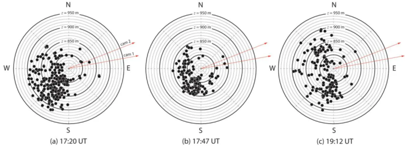
Characteristics of the explosions using 3D-analysis

346

Fig. 5 shows a 3D-view of the bomb trajectories through time for six eruptions that occurred on 347

October 5, 2012. The trajectories reveal the highly asymmetric ejection of the largest pyroclasts as a 348

function of time, the strong variability of jet directivity and of the maximum bomb heights among 349

eruptions over a period of 2 hours. Fig. 6 is a plot of the maximum elevation reached by the bombs 350

according to the azimuthal direction of their ejection. It illustrates the differences in direction and 351

intensity between the recorded explosions. Maximal ejection heights above the vent (about 755 m a.s.l.) 352

vary between 105 m (860 m in elevation) for the weakest eruption (i.e. 17:47) to 165 m (920 m in 353

elevation) for the strongest (i.e. 17:20). Maximum heights tend to be reached in the predominant ejection 354

direction (Fig. 6a, 6c) but exceptions occur (Fig. 6b). 355

11 357

Fig. 4 Comparison of the bomb velocities estimated using the 2D method (vertical plan passing by the 358

crater) and those calculated with the 3D reconstruction (eruption of 17:20, October 5, 2012). A and B 359

(and their respective colours) correspond to the bombs of Fig. 3 360

361

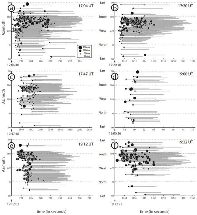
Fig. 7 links the azimuth of the ejection, the ejection time, the initial velocity (calculated in a further 362

section) and the trajectory duration. In Fig. 5d and 7d, it can be seen that during the small eruption at 363

19:00, bombs were ejected for a period of 2 s with no preferential azimuth. For the more energetic 364

eruption at 17:47 (Fig. 7c), the bombs were ejected over a wide azimuth range from south-east to north-365

west, although with an overall predominant direction towards the south-west (azimuth, N200). This 366

predominant direction of ejection was also visible during other high energy explosions (17:04, 17:20, 367

19:12 and 19:22). For example, bombs were ejected continuously for a period of 8 s at 17:04 and again 368

at 17:20 (Fig. 7a and 7b). These two eruptions were also characterized by an initial ejection of bombs 369

with no preferential azimuth for about 1 s, before becoming predominantly oriented to the south-west. 370

The eruption at 19:22 (Fig. 7f) began with an emission predominantly oriented towards the south-west 371

for the first 7s. Two seconds after the beginning of the eruption, a number of bombs were ejected in all 372

directions. When the bomb trajectories exhibit a high directivity, the highest bomb velocities tend to be 373

recorded in the predominant ejection direction. The eruption of 19:12 had two predominant directions 374

of ejection (Fig. 5e, 6c and 7e). The eruption began with an ejection of bombs in the same direction 375

(SW) as the other eruptions for 5 s. However, two seconds after the beginning of the eruption, another 376

preferential direction of ejection joined the first, in which bombs were ejected towards the north-west 377

for 2 s. This direction of emission was detected too for other eruptions but is less clear. It can be seen at 378

17:04 on Fig. 5a, with the two short pulses recorded at 17:47 on Fig. 7c (at t = 2841 s and t = 2843 s) 379

and with few bombs ejected at 17:20 (Fig. 5b and 7b). 380

381 382

12 383

Fig. 5 3D reconstruction of the trajectories of 6 explosions on October 5, 2012. The colours indicate the 384

time in seconds from the onset of the explosion. Black lines are parabolic fits of the trajectories 385 386

Discussion

Bomb modelling

To illustrate the potential of our 3D-reconstruction method, this section gives an example of the 390

parameters that can be deduced by comparing a simple ballistic model with our 3D-trajectories 391

reconstruction. Details of the model are presented in Online Resource 2. The model is simple and more 392

13

complex models have been developed (Taddeucci et al., 2017 and references therein). It is presented 393

here only to illustrate the possibilities given by the 3D-reconstruction of trajectories. Our model 394

calculates the bomb velocity from the Newton’s First Law and the drag force exerted by the atmosphere 395 on a bomb: 396





d

c

u

dt

   



v

g

v w

where t is time,

v





v v v

, ,



w





w w w

,

,



398

the relative velocity between the bomb and the air and g





399

spherical bomb, the parameter c is defined by: 400

3

8

c

C

r











with a the atmosphere density,  the bomb density, r its radius and Cd the drag coefficient

(Alatorre-402

Ibargüengoitia et al. 2012; Konstantinou, 2015). 403

By fitting the model to our 3D trajectories, we can estimate the three components of the bomb 404

velocity (vx, vy, vz) at the first detection (black dot in Fig. 8), the horizontal wind velocity (wx and wy)

405

and its orientation (w, azimuthal origin), and the coefficient c related to the atmospheric drag on the

406

bomb. Best fit estimations of these parameters were obtained by systematically varying the six 407

parameters and minimizing the standard deviation between the model and the observed trajectories in 408

both space and time. Fig. 8 shows a simulation of bomb B (see Fig. 3). For this bomb, the set of 409

parameters that reproduces the observed data (gray line, Fig. 8) are: vx=-7 m s-1, vy=-1.5 m s-1, vz=25.5

410

m s-1_{, c=0.0055 m}-1_{, w = 3.5 m s}-1_, 

w = -55° (wind from NW). The effects of misestimating the projection

411

positions of the bombs and the camera orientations are dominantly accommodated by translations of the 412

trajectories. This is why, even in the worst cases, the errors are low for the above values. They are 413

estimated to be less than 10% for velocities and the drag coefficient, by varying the bomb positions, the 414

camera angles and the lens distortion parameters with the normal laws of the 3D reconstruction section. 415

By using the values obtained for the parameters vx, vy, vz, c, w and w, and inverting the time, we

416

can determine the initial velocity and the initial direction of each bomb at the vent. The fitting between 417

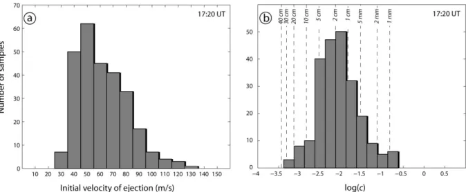
the measured trajectories and the model can be done automatically for all bombs detected during an 418

eruptive phase. Fig. 9a is a histogram of the initial bomb velocities of the 17:20 eruption. The majority 419

of the bombs were ejected at a velocity of 50 m s-1_{, with the velocities ranging from 30 to 130 m s}-1_{. At}

420

the crater where the bombs are ejected nearly vertically, the 3D characterisation improves only the 421

velocity estimation of less than 10% compared to 2D methods. The 3D method is, however, a powerful 422

tool for the estimation of ejection velocities if the bomb cannot be observed directly at the vent. 423

Modelling of the 3D-trajectories is also a powerful tool for estimating the drag of the bomb through 424

the air. To illustrate the sensitivity of the model to the parameter c, two other curves are added to the 425

initial curve (c=0.0055 m-1_{) on Fig. 8 with values of c = 0.01 m}-1 _{and c = 0.0025 m}-1_{. Fig. 9b is a}

426

histogram of the coefficient c calculated for all the bombs of the 17:20 eruption. The coefficient ranges 427

between 5×10-4 ₍₁₀-3.25_{) and 0.25 m}-1 ₍₁₀-0.6_{). To first order, the histogram can be used to estimate the}

428

size distribution of the bombs from Equation 5. If, for example, we assume a value of Cd=0.7, which

14

has been estimated for natural bombs (Alatorre-Ibargüengoitia and Delgado-Granados 2006; 430

de’Michieli Vitturi et al. 2010) and a bomb density of 1800 kg m-3 _{(e.g., Gurioli et al. 2013; Bombrun}

431

et al 2015; Lautze and Houghton 2007; Harris et al. 2013), a value of c = 10-3 _m-1 _{corresponds to a radius}

432

of 14.6 cm. The bomb radii corresponding to Cd = 0.7 and  = 1800 kg m-3 are plotted on Fig. 9b. They

433

range between <1 mm and >30 cm. Note that, below 64 mm down to 2 mm, the term lapilli must be 434

used instead of bomb, and ash below 2 mm. It should also be pointed out that it seems unlikely for the 435

smallest size particles of the histogram (in particular ash < 1 mm) to be sufficiently radiative to be 436

detectable with a pixel size (i.e., a ground sample distance) of 20 cm. The sizes given are dependent on 437

the assumptions about the bomb/lapilli density and the drag coefficient. A particle with a low density, 438

and a complex shape and roughness might show the same coefficient c as a smaller particle with the 439

density chosen and the spherical shape used for the example. A strong deceleration, comparable to that 440

of a small particle, can also be observed for a larger particle leaving a gas jet above the crater. Our 441

method of 3D-reconstruction can be used with more complete numerical models that would take into 442

account these parameters. 443

444

Fig. 6: Maximal elevation reached by the bombs and azimuthal direction of ejections. The elevation of 445

the NE crater in October 2012 was about 755 m a.s.l. The graphics show that the bombs were essentially 446

ejected in a SW direction. The eruption at 19:12 was characterized by a significant amount of ejecta to 447

the NW, a direction that is rare or absent from the other eruptions 448

449

Limitations and improvements for the method

450

In the future, the number of trajectories detected by our methodology can be improved by 451

improving the camera resolution and frame rates. For example, more than 3000 trajectories were 452

detected for each camera, but fewer than 300 bombs were identified unambiguously. The use of higher 453

resolution cameras would improve the precision of the bomb locations, would give more precise 454

estimation of the bomb size and would reduce bomb identification uncertainties. Higher frame rates, 455

using high speed cameras, would also reduce uncertainties of bomb recognition and facilitate trajectory 456

reconstruction for each camera because bomb positions would be very close on successive images. With 457

more confidence in the recognition, selection criteria that reject some trajectories could be lowered. This 458

would allow complex trajectories, such as those induced by bomb collisions, to be detected 459

unambiguously (Vanderkluysen et al. 2012). Another parameter that could be improved is the dynamics 460

of the sensor. The challenge is to be able to see the bombs in the first phase of the eruption, when the 461

number of hot bombs is high and tends to saturate the sensor. However, if the sensitivity is too low, the 462

15

bombs that cool rapidly are not detectable. With the cameras used, it was possible to acquire images 463

with a higher dynamic range, for example 12 or 16 bytes. However, this would have produced a very 464

high flux of data to be transmitted and recorded (55 to 73 Mb/s), which exceeded the capability of the 465

laptop used during fieldwork. Finally, the system could be improved by using more than two 466

synchronized cameras around the area under observation. This would combine the advantages of easier 467

recognition of similar bombs with the accuracy related to a wider angle of view and would highly 468

improve bomb recognition. 469

470

Fig. 7 Azimuth of the bomb ejection against time for the six eruptions studied on Oct. 5 2012. The 471

horizontal axis is the time in seconds (a-c from 17:00 UT, and d-f from 19:00 UT). The black dots 472

indicate the ejection time of each bomb and their size indicates the initial ejection velocity (see inset in 473

7a). The grey lines represent the time-period of the reconstructed trajectories (up to the point the bombs 474

reach the ground, are masked by the topography or are too cooled to be detected) 475

16 476

Fig. 8 Measurement of the 3D trajectory of bomb B (in grey; cf. Fig. 3) and simulations (in black) for 3 477

values of c (see Equation 8). The data are fitted in space (a, d) and time (b, c). The dashed line 478

corresponds to the extrapolation of the bomb trajectory from its first detected position back to the vent 479

using the best-fit values 480

481

482

Fig. 9 (a) Histogram of calculated initial ejection velocities at the vent for the 230 bombs trajectories 483

reconstructed during the 17:20 eruption using the model and its extrapolation. (b) Apparent drag 484

coefficient c calculated using the model. The vertical lines indicate the radii corresponding to the values 485

of c for Cd=0.7 and a bomb density of 1800 kg m-3

17 487

Contribution of 3D reconstruction for conduit processes

488

The computed trajectories for six eruptions show a preferential direction of ejection to the south-489

west. It could be argued that such a direction, away from the camera, could be an artefact. Bombs ejected 490

parallel to the line between the vent and the cameras could be more difficult to identify because of their 491

location in the brightest area above the vent, potentially causing larger errors on their trajectories. To 492

check if the calculated direction is correct, we have also taken photos of the same vent from the summit 493

of Stromboli (Fig. 2). From this view angle perpendicular to the view angles of the cameras, the direction 494

of ejection calculated, towards the south-west, is clearly confirmed (Fig. 10). 495

496

497

Fig. 10 Photograph of the eruption at 12:56 UT (Oct. 5, 2012); taken from the south-east (Pizzo) showing 498

that the ejection is oriented to the SW (location of the photo on Fig. 2) 499

500

Our method might also be a useful tool for understanding conduit processes. It shows that, during 501

the period studied, the direction of bomb ejection was either uni-directional or multi-directional and that 502

it varied over time during an eruption and among eruptions within timescales of tens of minutes. For the 503

eruptions at 17:04 and 17:20, the first bombs were ejected with relatively slow velocities (50 – 100 m s

-504

1_{) and in all directions (Fig. 7 a,b). The emissions then evolved to higher velocities with a predominant}

505

direction of ejection (N200). This is compatible with a slug of gas that reached the surface (James et al., 506

2004; Leduc et al., 2015). The explosions initially occurred close to the surface and they ejected bombs 507

radially. Afterwards, the successive explosions might have become progressively deeper, and more 508

18

influenced by the orientation of the magma conduit, which seems to have been oriented N200 with a dip 509

of about 75° (95% of the trajectories lie between 60° and 85°) during our field campaign. These values 510

are compatible with the inclinations obtained from the locations of VLP seismic events (Chouet et al., 511

2008a) even if the comparison is limited by the strong morphological changes that have affected the 512

crater area within 15 years separating our field campaigns. The smallest eruptions at 17:47 and 19:00 513

correspond to superficial explosions, compatible with the radial directions of the bombs. However, it 514

appears that even during small and superficial eruptions the gas pressure can be high, based on the high 515

velocities recorded at 19:00. 516

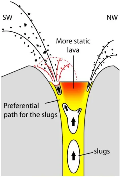
The eruption at 19:12 provides a more complete view of the superficial geometry. It began by two 517

directions of ejection followed by a radial emission. The two directions of ejection, recorded to a lesser 518

extent at 17:04 (Fig. 5a), can hardly be explained by a simple conduit geometry. The explanation could 519

be that the directions of the explosions are controlled by the rheology of the superficial magma and its 520

spatial distribution. The upper part of the conduit may be clogged by pyroclasts (Capponi et al., 2016) 521

and is probably filled with a mixture of vesicular and denser, partially crystallized and degassed magma 522

(e.g. Lautze and Houghton 2007; Burton et al. 2007; Bai et al. 2011; Gurioli et al. 2014). The latter can 523

form static zones representing more difficult pathways, so that the preferential path of the rising slugs 524

would be around the edges of the degassed magma zones. An upper conduit that broadened towards the 525

surface, the top of which is partially obstructed by lava clots recycled from previous explosions in 526

variable amount and conditions, might explain how explosions could occur simultaneously in many 527

different orientations (Fig. 11). Perturbations of the static magma, rising of other slugs, or variations in 528

the slug properties (viscosity, gas content) downwards could explain how a radial explosion occurred 3 529

s after the beginning of the directed explosions. 530

531

Conclusion

532

We have developed a system of synchronised cameras for the automated reconstruction of hundreds of 533

volcanic bomb trajectories in 3D in space plus time. The synchronization, done by connecting the 534

cameras to the same computer, is essential for the study of high velocity phenomena. The reconstructed 535

trajectories, coupled with a ballistic model, allows deduction of bomb particle sizes (given shape and 536

density assumption) from their drag coefficients and to calculate their initial velocities at the vents as 537

well as their directions of ejection. Alternatively, if particle size is known, the drag coefficient can be 538

used to solve for shape and/or density. The trajectories reveal the time and space variations in velocities 539

and directions within single explosive events as well as between successive explosions. Their 540

interpretation is compatible with preferential paths of slugs, which can become focused at the edges of 541

the upper part of the conduit probably due to formation of a central viscous cap. Our method thus 542

represents a tool allowing insights into superficial magmatic conditions and their relation with particle 543

dynamics. It also provides calibration data for future techniques developed for emission dynamics 544

characterisation, such as the Doppler radar method (Gouhier and Donnadieu, 2008). 545

19 547

Fig. 11 A possible scheme of the upper conduit of Stromboli compatible with the bomb trajectories 548

observed. Radial ejections (red) can be explained by explosions near the surface. With time, the slug 549

bursts at increasing depth, focusing the directions of ejections. The various directions observed may 550

indicate heterogeneities in the magma rheology that can form more than a single path for the slugs 551

552

Acknowledgements

553

The multidisciplinary mission was funded by the Laboratory of Excellence ClerVolc (contribution 554

number 393), the Chaire d’Excellence de la region Auvergne and the Observatoire de Physique du 555

Globe de Clermont-Ferrand. The development of the stereoscopic system was funded by the

556

Volcanology group at the Laboratoire Magmas et Volcans. We thank JL Piro for sharing his experience 557

on camera synchronisation and F Jabet, director of the Airylab company (http://airylab.fr/), for his 558

readiness to help and for having modified the Genika trigger software for our needs. We thank S. Valade, 559

M. Bombrun, G. Sawyer, C. Hervier, the italian DPC and Helijet for their help in the field. The 560

manuscript was improved by the relevant comments of two anonymous reviewers and of the Associate 561

Editor, M. R. James. 562

20

References

564

Alatorre-Ibargüengoitia MA, Delgado-Granados H (2006) Experimental determination of drag coefficient for

565

volcanic materials: calibration and application of a model to Popocatépetl volcano (Mexico) ballistic projectiles.

566

Geophys Res Lett 33:11. https://doi.org/10.1029/2006GL026195

567

Alatorre-Ibargüengoitia MA, Delgado-Granados H, Dingwell DB (2012) Hazard map for volcanic ballistic impacts

568

at Popocatépetl volcano (Mexico). Bull Volcanol 74: 2155–2169. https://doi.org/10.1007/s00445-012-0657-2

569

Bai L, Baker DR, Polacci M, Hill RJ (2011) In-situ degassing study on crystal-bearing Stromboli basaltic magmas:

570

Implications for Stromboli explosions. Geophys Res Lett 38, L17309. https://doi.org/10.1029/2011GL048540.

571

Bombrun M, Barra V, Harris A (2014) Algorithm for particle detection and parameterization in high-frame-rate

572

thermal video. J Appl Remote Sens 8 (1), 083549. https://doi.org/10.1117/1.JRS.8.083549

573

Bombrun M, Harris AJL, Gurioli L, Battaglia J, Barra V (2015) Anatomy of a Strombolian eruption: Inferences

574

from particle data recorded with thermal video. J Geophys Res Solid Earth 120: 2367–2387.

575

https://doi.org/10.1002/2014JB011556

576

Brown DC (1966) Decentering distortion of lenses, Photogrammetric Engineering, 32 (3) 444–462.

577

Burton MR, Mader HM, Polacci M (2007) The role of gas percolation in quiescent degassing of persistently active

578

basaltic volcanoes. Earth Planet Sci Lett 264: 46–60. https://doi.org/10.1016/j.epsl.2007.08.028

579

Capponi A, Taddeucci J, Scarlato P, Palladino DM (2016) Recycled ejecta modulating Strombolian explosions.

580

Bull Volcanol 78, 13. https://doi.org/10.1007/s00445-016-1001-z

581

Chevalier L, Donnadieu F (2015) Considerations on ejection velocity estimation from infrared radiometer data: a

582

case study at Stromboli volcano. J Volcanol Geotherm Res 302:130-140.

583

https://doi.org/10.1016/j.jvolgeores.2015.06.022

584

Chouet B, Hamisevicz N, McGetchin TR (1974) Photoballistics of volcanic jet activity at Stromboli, Italy. J

585

Geophys Res 79 (32) 4961–4976. https://doi.org/10.1029/JB079i032p04961

586

Chouet B, Dawson P, Martini M (2008a) Upper conduit structure and explosion dynamics at Stromboli. In: Calvari

587

S, Inguaggiato S, Puglisi G, Ripepe M, Rosi M (eds) The Stromboli volcano: an integrated study of the 2002–2003

588

eruption. AGU, Washington, pp 81–92. https://doi.org/10.1029/182GM08

589

Chouet B, Dawson P, Martini M (2008b) Shallow-conduit dynamics at Stromboli Volcano, Italy, imaged from

590

waveform inversions, S.J. Lane, J.S. Gilbert (Eds.), Fluid Motions in Volcanic Conduits: A Source of Seismeic

591

and Acoustic Signals, Vol. 307 of Geol. Soc. Spec. Publ., The Geological Society, pp. 57-84.

592

https://doi.org/10.1144/SP307.5

593

Crocker JC, Grier DG (1996) Methods of Digital Video Microscopy for Colloidal Studies. J Colloid Interface Sci

594

179, 298. https://doi.org/10.1006/jcis.1996.0217

595

de'Michieli Vitturi M, Neri A, Esposti Ongaro T, Lo Savio S, Boschi E (2010) Lagrangian modeling of large

596

volcanic particles: Application to Vulcanian explosions. J Geophys Res Solid Earth 115: B8.

597

https://doi.org/10.1029/2009JB007111

598

Diefenbach AK, Crider JG, Schilling SP, Dzurizin D (2012) Rapid, low-cost photogrammetry to monitor volcanic

599

eruptions: an example from Mount St. Helens, Washington, USA. Bull Volcanol 74: 579.

600

https://doi.org/10.1007/s00445-011-0548-y

601

Eiken T, Sund M (2012) Photogrammetric methods applied to Svalbard glaciers: accuracies and challenges. Polar

602

Res., 31, 18671. https://doi.org/10.3402/polar.v31i0.18671

603

Eltner A, Kaiser A, Abellan A, Schindewolf M (2017) Time lapse structure from motion photogrammetry for

604

continuous geomorphic monitoring. Earth Surf. Process. Landforms, 42(14): 2240-2253.

605

https://doi.org/10.1002/esp.4178

606

Favalli M, Fornaciai A, Pareschi MT (2009) LIDAR strip adjustment: Application to volcanic areas.

607

Geomorphology 111: 123–135. https://doi.org/10.1016/j.geomorph.2009.04.010

21

Formenti Y, Druitt TH, Kelfoun K (2003) Characterisation of the 1997 Vulcanian explosions of Soufrière Hills

609

Volcano, Montserrat, by video analysis. Bull Volcanol 65(8):587–605.

https://doi.org/10.1007/s00445-003-0288-610

8

611

Gaudin D, Moroni M, Taddeucci J, Scarlato P (2014) Pyroclast Tracking Velocimetry: A particle tracking

612

velocimetry-based tool for the study of Strombolian explosive eruptions. J Geophys Res: Solid Earth 119 (7),

613

5369–5383. https://doi.org/10.1002/2014JB011095

614

Gaudin D, Taddeucci J, Houghton BF, Orr TR, Andronico D, Del Bello E, Kueppers U, Ricci T, Scarlato P (2016)

615

3-D high-speed imaging of volcanic bomb trajectory in basaltic explosive. Geochem Geophys Geosyst 17 (10):

616

4268–4275. https://doi.org/10.1002/2016GC006560

617

Gaudin D, Taddeucci J, Scarlato P, del Bello E, Ricci T, Orr T, Houghton B, Harris A, Rao S, Bucci A (2017)

618

Integrating puffing and explosions in a general scheme for Strombolian-style activity, J. Geophys. Res. Solid Earth,

619

122, 1860–1875. https://doi.org/10.1002/2016JB013707

620

Gouhier M, Donnadieu F (2008) Mass estimations of ejecta from Strombolian explosions by inversion of

Doppler-621

radar measurements. J. Geophys. Res., 113, B10202. https://doi.org/10.1029/2007JB005383

622

Granshaw SI (1980) Bundle adjustment methods in engineering photogrammetry. Photogrammetric record,

623

10(56): 181:207. https://doi.org/10.1111/j.1477-9730.1980.tb00020.x

624

Granshaw, S.I. (2016) Photogrammetric terminology.Photogrammetric Record, 31(154), 210-252.

625

https://doi.org/10.1111/phor.12146

626

Gurioli L, Harris AJL, Colò L, Bernard J, Favalli M, Ripepe M, Andronico D (2013) Classification, landing

627

distribution, and associated flight parameters for a bomb field emplaced during a single major explosion at

628

Stromboli, Italy. Geology 41, 5: 559–562. https://doi.org/10.1130/G33967.1

629

Gurioli L, Colò L, Bollasina AJ, Harris AJL, Whittington A, Ripepe M (2014) Dynamics of Strombolian

630

explosions: Inferences from field and laboratory studies of erupted bombs from Stromboli volcano. J Geophys Res

631

Solid Earth 119: 319–345. https://doi.org/10.1002/2013JB010355

632

Harris AJL, Ripepe M (2007) Synergy of multiple geophysical approaches to unravel explosive eruption conduit

633

and source dynamics−A case study from Stromboli. Geochem 67: 1–35.

634

https://doi.org/10.1016/j.chemer.2007.01.003

635

Harris AJL, Ripepe M, Calvari S, Lodato L, Spampinato L (2008) The 5 April 2003 explosion of Stromboli: timing

636

of eruption dynamics using thermal data. In: Calvari S, Inguaggiato S, Puglisi G, Ripepe M, Rosi M (eds) The

637

Stromboli volcano: an integrated study of the 2002–2003 eruption. AGU, Washington, pp 305–316.

638

https://doi.org/10.1029/182GM25.

639

Harris AJL, Valade S, Sawyer G, Donnadieu F, Battaglia J, Gurioli L, Kelfoun K, Labazuy P, Stachowicz T,

640

Bombun M, Barra V, Delle Donne D, Lacanna G (2013) Modern Multispectral Sensors Help Track Explosive

641

Eruptions. EOS 94, 37:321–322. https://doi.org/10.1002/2013EO370001

642

James MR, Lane SJ, Chouet BA, Gilbert JS (2004) Pressure changes associated with the ascent and bursting of

643

gas slugs in liquid-filled vertical and inclined conduits. J Volcanol Geotherm Res 129, 1–3, 61–82.

644

https://doi.org/10.1016/S0377-0273(03)00232-4

645

James MR, Robson H (2014) Sequential digital elevation models of active lava flows from ground-based stereo

646

time-lapse imagery. ISPRS J. Photogram. Remote Sens., 97, 160-170.

647

https://doi.org/10.1016/j.isprsjprs.2014.08.011

648

James T, Murray T, Selmes N, Scharrer K, O’Leary M (2014) Buoyant flexure and basal crevassing in dynamic

649

mass loss at Helheim Glacier. Nature Geoscience, 7. https://doi.org/10.1038/ngeo2204

650

Konstantinou KI (2015) Maximum horizontal range of volcanic ballistic projectiles ejected during explosive

651

eruptions at Santorini caldera. J Volcanol Geotherm Res 301: 107–115.

652

https://doi.org/10.1016/j.jvolgeores.2015.05.012

653

Lautze NC, Houghton BF (2007) Linking variable explosion style and magma textures during 2002 at Stromboli

654

volcano, Italy. Bull Volcanol 69, 4: 445–460, https://doi.org/10.1007/s00445-006-0086-1