HAL Id: hal-03008649
https://hal.archives-ouvertes.fr/hal-03008649
Submitted on 16 Nov 2020
HAL is a multi-disciplinary open access
archive for the deposit and dissemination of
sci-entific research documents, whether they are
pub-lished or not. The documents may come from
teaching and research institutions in France or
abroad, or from public or private research centers.
L’archive ouverte pluridisciplinaire HAL, est
destinée au dépôt et à la diffusion de documents
scientifiques de niveau recherche, publiés ou non,
émanant des établissements d’enseignement et de
recherche français ou étrangers, des laboratoires
publics ou privés.
Lupus DANCe
P. A. B. Galli, H. Bouy, J. Olivares, N. Miret-Roig, R. G. Vieira, L. M. Sarro,
D. Barrado, A. Berihuete, C. Bertout, E. Bertin, et al.
To cite this version:
P. A. B. Galli, H. Bouy, J. Olivares, N. Miret-Roig, R. G. Vieira, et al.. Lupus DANCe: Census of
stars and 6D structure with Gaia-DR2 data. Astronomy and Astrophysics - A&A, EDP Sciences,
2020, 643, pp.A148. �10.1051/0004-6361/202038717�. �hal-03008649�
https://doi.org/10.1051/0004-6361/202038717 c P. A. B. Galli et al. 2020
Astronomy
&
Astrophysics
Lupus DANCe
Census of stars and 6D structure with Gaia-DR2 data
?P. A. B. Galli
1, H. Bouy
1, J. Olivares
1, N. Miret-Roig
1, R. G. Vieira
2, L. M. Sarro
3, D. Barrado
4, A. Berihuete
5,
C. Bertout
6, E. Bertin
6, and J.-C. Cuillandre
71 Laboratoire d’Astrophysique de Bordeaux, Univ. Bordeaux, CNRS, B18N, allée Geoffroy Saint-Hillaire, 33615 Pessac, France e-mail: [email protected]
2 Departamento de Física, Universidade Federal de Sergipe, São Cristóvão, SE, Brazil 3 Depto. de Inteligencia Artificial, UNED, Juan del Rosal, 16, 28040 Madrid, Spain
4 Centro de Astrobiología, Depto. de Astrofísica, INTA-CSIC, ESAC Campus, Camino Bajo del Castillo s/n, 28692 Villanueva de la Cañada, Madrid, Spain
5 Dept. Statistics and Operations Research, University of Cádiz, Campus Universitario Río San Pedro s/n, 11510 Puerto Real, Cádiz, Spain
6 Institut d’Astrophysique de Paris, CNRS UMR 7095 and UPMC, 98bis bd Arago, 75014 Paris, France 7 AIM Paris Saclay, CNRS/INSU, CEA/Irfu, Université Paris Diderot, Orme des Merisiers, France Received 22 June 2020/ Accepted 21 September 2020
ABSTRACT
Context.Lupus is recognised as one of the closest star-forming regions, but the lack of trigonometric parallaxes in the pre-Gaia era hampered many studies on the kinematic properties of this region and led to incomplete censuses of its stellar population.
Aims.We use the second data release of the Gaia space mission combined with published ancillary radial velocity data to revise the census of stars and investigate the 6D structure of the Lupus complex.
Methods.We performed a new membership analysis of the Lupus association based on astrometric and photometric data over a field of 160 deg2around the main molecular clouds of the complex and compared the properties of the various subgroups in this region.
Results.We identified 137 high-probability members of the Lupus association of young stars, including 47 stars that had never been reported as members before. Many of the historically known stars associated with the Lupus region identified in previous studies are more likely to be field stars or members of the adjacent Scorpius-Centaurus association. Our new sample of members covers the magnitude and mass range from G ' 8 to G ' 18 mag and from 0.03 to 2.4 M , respectively. We compared the kinematic properties of the stars projected towards the molecular clouds Lupus 1–6 and showed that these subgroups are located at roughly the same distance (about 160 pc) and move with the same spatial velocity. Our age estimates inferred from stellar models show that the Lupus subgroups are coeval (with median ages ranging from about 1 to 3 Myr). The Lupus association appears to be younger than the population of young stars in the Corona-Australis star-forming region recently investigated by our team using a similar methodology. The initial mass function of the Lupus association inferred from the distribution of spectral types shows little variation compared to other star-forming regions.
Conclusions.In this paper, we provide an updated sample of cluster members based on Gaia data and construct the most complete picture of the 3D structure and 3D space motion of the Lupus complex.
Key words. open clusters and associations: individual: Lupus – stars: formation – stars: distances – methods: statistical – parallaxes – proper motions
1. Introduction
The Lupus molecular cloud complex is one of the closest and largest low-mass star-forming regions of the southern sky. It con-sists of several subgroups associated with different molecular clouds labelled as Lupus 1–9 that exhibit distinct morphologies as revealed by CO surveys and extinction maps (Hara et al. 1999;
Cambrésy 1999; Tachihara et al. 2001; Dobashi et al. 2005). Although they are part of the same complex, Lupus clouds dif-fer significantly regarding their star formation activity. Some clouds have dense concentrations of T Tauri stars (e.g. Lupus 3) while others (e.g. Lupus 7–9) display no signs of ongoing star formation (Comerón 2008).
?
Full Tables A.1–A.4 are only available at the CDS via anony-mous ftp to cdsarc.u-strasbg.fr(130.79.128.5) or viahttp: //cdsarc.u-strasbg.fr/viz-bin/cat/J/A+A/643/A148
Early surveys leading to the identification of Lupus stars mostly focused on the molecular clouds with active star for-mation (i.e. Lupus 1–4), but more recently a few young stel-lar objects (YSOs) have also been discovered in Lupus 5 and 6 (Manara et al. 2018;Melton 2020). Most of the hitherto known classical T Tauri stars (CTTSs) in Lupus were identified by
Schwartz(1977) andHughes et al.(1994) based on their strong Hα and infrared excess emissions. Succeeding studies identified a more dispersed and older population of weak-emission line T Tauri stars (WTTSs) from ROSAT X-ray pointed observations surrounding the Lupus clouds, which greatly exceed the num-ber of CTTSs located in the immediate vicinity of the molecu-lar clouds (Krautter et al. 1997;Wichmann et al. 1997a,b). The census of Lupus stars was later expanded byMerín et al.(2008) based on infrared observations collected with the Spitzer Space Telescope as part of the cores to disk (c2d) legacy project. In
Open Access article,published by EDP Sciences, under the terms of the Creative Commons Attribution License (https://creativecommons.org/licenses/by/4.0),
a subsequent study,Comerón et al.(2009) revealed a new pop-ulation of cool stars and brown dwarfs potentially associated with Lupus based on their spectral energy distributions (SEDs) derived from optical and infrared photometry.López Martí et al.
(2011) confirmed most of these sources to be genuine mem-bers of the Lupus region based on their proper motions and showed the importance of using kinematic information (e.g. proper motions, parallaxes, and radial velocities) to assess mem-bership.
The distance to Lupus has undergone several revisions and has become a matter of debate in the recent decades although it has always been recognised as one of the closest star-forming regions to the Sun. Distance determinations in the literature range from 100 pc (Knude & Hog 1998) to 360 pc (Knude & Nielsen 2001). Franco (1990) and Hughes et al.
(1993) estimated the distances of 165 ± 15 pc and 140 ± 20 pc, respectively, based on the interstellar reddening of field stars.
Lombardi et al. (2008) used a more robust method based on 2MASS wide field extinction maps and derived the distance of 155 ± 8 pc with a depth of 51+61−35pc, which the authors explained as the Lupus clouds being at different distances. It is important to mention that these distances are only average estimates based on indirect methods because distances for individual stars derived from trigonometric parallaxes existed (until recently) for only a few stars in this region. For example,Bertout et al.(1999) used trigonometric parallaxes of five stars from the
Hipparcos
cat-alogue (ESA 1997) to estimate the distance to Lupus. Three of them, which are associated with Lupus 1, 2 and 4 have a mean parallax of $= 6.79 ± 1.50 mas that roughly defines a distance of 147+42−27pc. The other two stars, located in Lupus 3, have a mean parallax of $ = 4.38 ± 0.67 mas, which puts this cloud much farther away at a distance of 228+41−30pc. Alternatively, kine-matic distances to individual stars in this region were derived in the past from the convergent point method under the assumption that the Lupus stars are comoving (Makarov 2007;Galli et al. 2013). The resulting distances confirmed the important depth effects (i.e. distance variations along the line of sight) reported in previous studies.Lupus is located between the Upper Scorpius (US) and Upper Centaurus-Lupus (UCL) subgroups of the Scorpius-Centaurus (Sco-Cen) association, but despite the close proxim-ity in the sky it represents a more recent star formation episode in this region (Preibisch et al. 2008). In this context, the exis-tence of a more dispersed and older population of WTTSs near the Lupus clouds as reported in previous studies is not sur-prising, but their association with the younger population con-centrated in the immediate vicinity of the molecular clouds needs to be confirmed. The second data release of the Gaia space mission (Gaia-DR2, Gaia Collaboration 2018) provides the best astrometry available to date to further assess the mem-bership of the historically known members. When combined with radial velocity information these data can be used to con-strain not only the 3D positions of the stars, but also their 3D space motions. The stellar content of the Sco-Cen associ-ation was recently revised by Damiani et al. (2019) based on Gaia-DR2 data, but a dedicated study of the Lupus clouds is still missing in the literature. The proper motions and paral-laxes in the Gaia-DR2 catalogue are more precise by one or two orders of magnitude compared to the ground-based astrom-etry used in previous studies of the Lupus region (see e.g.
Makarov 2007;López Martí et al. 2011; Galli et al. 2013), and they will therefore allow us to obtain a clean sample of members and a more accurate picture of the overall 6D structure of the complex.
This paper is one in a series as part of the Dynamical Analy-sis of Nearby Clusters project (DANCe,Bouy et al. 2013). Here, we investigate the census of stars and kinematic properties of the Lupus association of young stars based on Gaia-DR2 data. It is organised as follows. In Sect.2we compile the list of Lupus stars from previous studies in the literature that is used in Sect.3to perform a new membership analysis based on a novel method-ology developed by our team (Sarro et al. 2014;Olivares et al. 2019). In Sect.4we revisit several properties of the Lupus sub-groups (e.g. distance, spatial velocity, age, spatial distribution, and initial mass function) based on our new sample of cluster members. Finally, we summarise our conclusions in Sect.5. 2. Sample of Lupus stars from previous studies We construct our initial sample of stars based on the lists of members and candidate members that have been associ-ated with the Lupus star-forming region in previous studies. We take the samples of (i) 73 stars fromHughes et al. (1994), (ii) 136 stars from Krautter et al. (1997), (iii) 92 stars from
Wichmann et al. (1997a), (iv) 48 stars from Wichmann et al.
(1997b), (v) 159 stars from Merín et al. (2008), (vi) 248 stars from Tables 4 and 9 ofComerón et al.(2009), (vii) 82 stars from Tables 2 and 4 ofLópez Martí et al.(2011), and (viii) 69 stars fromDamiani et al.(2019). This results in a sample of 508 stars after removing the sources in common among the several lists of Lupus stars. We find proper motions and parallaxes for 441 stars of this sample in the Gaia-DR2 catalogue. Figure1shows the location of the stars in this sample with respect to the main star-forming clouds of the Lupus complex. We use the boundaries defined in Fig. 3 ofHara et al.(1999) to assign the sources in the Lupus sample to the corresponding molecular cloud of the com-plex based on their sky positions. This procedure does not con-firm membership to the corresponding clouds, but allows us to compare the stellar proper motions of the stars projected against the various clouds. As discussed in Sect. 1, it is apparent that the stars identified byKrautter et al.(1997) andWichmann et al.
(1997a,b) constitute a more dispersed “off-cloud” population that surrounds the molecular clouds.
Similarly, we compile a list of known members of the adja-cent Sco-Cen association that will be used in the forthcom-ing discussion. We restrict this sample to the to stars in the UCL subgroup that are located in the general region of the main star-forming clouds of the Lupus complex (334◦< l < 342◦
and 5◦< b < 25◦). Our UCL sample is based on the lists of sources previously identified in this region by de Zeeuw et al.
(1999), Preibisch et al. (2008), Pecaut & Mamajek (2016) and
Damiani et al. (2019). It includes1352 stars with measured proper motions and parallaxes in the Gaia-DR2 catalogue.
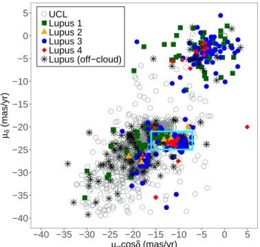
Figure 2 shows the distribution of proper motions for the Lupus and UCL stars compiled from the literature. This prelimi-nary analysis reveals the existence of (at least) three populations of stars in the Lupus sample from the literature. First, there is a background population of sources projected towards Lupus 1, 3, and 4 with proper motions typically smaller than 10 mas yr−1
which are more likely to be unrelated to the Lupus star-forming region as anticipated in past studies (López Martí et al. 2011;
Galli et al. 2013). Second, there is a more diffuse population of stars with proper motions that overlap with the UCL stars in this region of the sky. Indeed, many of them have been identified as Sco-Cen members in the recent study conducted by Damiani et al. (2019). Finally, we note an overdensity of stars around (µαcos δ, µδ) ' (−11, −23) mas yr−1 (see high-lighted region in Fig.2) including stars projected towards the
Fig. 1. Location of the Lupus stars identified in previous studies overlaid on the extinction map ofDobashi et al.
(2005) in Galactic coordinates. Colours and symbols denote the samples of stars from each study. The red dashed lines indicate the position of the main molec-ular clouds defined byHara et al.(1999).
four molecular clouds of the complex (Lupus 1–4) and with proper motions consistent with membership in Lupus (see e.g.
Galli et al. 2013). The latter will be used in our forthcoming analysis (see Sect. 3) to search for additional members to the Lupus association and investigate the kinematic properties of this star-forming region.
3. Membership analysis
The membership analysis performed in this study for the Lupus star-forming region is based on the methodology developed by
Sarro et al.(2014) andOlivares et al.(2019). The main steps of our analysis are briefly summarised in this section and we refer the reader to the original papers for further details.
First, we define the representation space of our member-ship analysis (i.e. the set of observables) that we use to classify the sources as cluster members or field stars. The represen-tation space includes both astrometric and photometric fea-tures of the stars given in the Gaia-DR2 catalogue. It does not include sky positions since the Lupus association is spread over a relatively large sky region without any clear over-density with respect to the field population in terms of stellar posi-tions (see Fig.1). In our case the inclusion of stellar positions in the representation dilutes the discriminant power of paral-laxes, proper motions and photometry in the membership anal-ysis, thus resulting in higher contamination rates. Furthermore, we do not use the blue photometry (BP) from Gaia-DR2 due
to some inconsistencies reported in the literature in the BP sys-tem (see e.g.Maíz Apellániz & Weiler 2018). We measured the relative importance of the photometric features using a random-forest classifier and concluded that GRP is a more discriminant
magnitude than G for identifying members. So, our representa-tion space for the membership analysis is defined by µαcos δ, µδ, $, GRP, and G − GRP.
The region of the sky downloaded from the Gaia-DR2 cata-logue to perform our membership analysis is defined by 334◦ ≤
l ≤342◦ and 5◦ ≤ b ≤ 25◦ to include the molecular clouds of
the complex with active star formation (Lupus 1–4). This input catalogue contains 14 471 847 sources (10 470 632 of them with complete data in the chosen representation space) whose mem-bership status with respect to the Lupus region will be investi-gated in our analysis.
We modelled the field population using Gaussian Mixture Models (GMM)1. The field model was computed only once at the beginning of our membership analysis and held fixed during the process. We tested field models with 20, 40, 60, 80, 100, 120, 140 and 160 components, and inferred their parameters using a random sample of 106 sources from our input catalogue. We
compute the Bayesian information criteria (BIC) for each one of the models and take the one (with 80 components) that returns the minimum BIC value as the optimum model for our analysis.
1 A Gaussian Mixture Model is a model that describes a probability distribution as a linear combination of k Gaussian distributions, where kis the number of components.
● ● ● ● ● ● ● ● ● ● ● ● ● ● ● ● ● ● ● ● ● ● ● ● ● ● ●● ● ● ● ● ● ● ● ● ● ● ●● ● ●● ● ● ● ● ●● ●● ● ● ● ● ● ● ● ● ● ● ● ● ● ● ● ● ● ● ● ● ● ● ● ● ● ● ● ● ● ●● ● ● ● ● ● ● ● ● ● ● ● ● ● ● ● ● ● ● ●● ● ● ●● ● ● ● ● ● ● ● ● ● ●● ● ● ● ● ●● ● ● ● ● ● ● ● ● ● ● ● ● ● ● ● ● ● ● ● ● ● ● ● ● ●● ● ● ● ● ● ● ● ● ● ● ● ●● ● ● ● ● ● ● ● ● ● ● ● ● ● ● ● ● ● ● ● ● ●●● ● ● ● ● ● ●● ● ● ● ● ● ● ● ● ● ● ● ● ● ● ● ● ● ● ● ● ● ●● ● ● ● ● ● ● ● ● ● ●● ● ●●● ● ● ● ● ● ● ● ● ● ● ● ● ●● ● ● ● ● ● ● ● ● ● ● ●● ● ● ● ● ● ● ● ● ● ● ● ● ● ● ● ● ● ● ● ● ● ● ● ● ● ● ● ● ● ● ● ● ● ● ● ● ● ● ● ● ● ● ● ● ● ● ● ● ● ●● ●● ● ●● ● ● ● ● ● ● ● ● ● ● ● ● ●● ● ● ● ● ● ● ● ● ● ● ● ● ● ● ● ● ●● ● ● ● ● ● ● ● ● ●● ● ●● ● ● ● ● ● ● ● ● ● ● ● ● ● ● ● ● ● ● ● ● ● ● ● ● ● ● ● ● ● ● ●●● ● ● ● ●● ● ● ● ● ● ● ● ● ● ● ● ● ● ● ● ● ● ●● ● ● ● ● ● ● ● ● ● ● ● ● ● ● ● ● ● ● ● ● ● ● ● ● ● ● ● ● ● ● ● ● ● ● ● ●● ● ● ● ● ● ● ● ● ● ● ● ● ● ● ● ● ● ● ● ● ● ● ●● ● ● ● ● ● ● ● ● ● ● ● ● ● ● ● ● ●● ● ● ● ● ● ● ● ● ● ● ● ● ● ● ● ● ● ● ● ● ● ● ● ● ● ● ● ● ● ● ● ● ● ● ● ●● ● ● ● ● ● ● ● ● ● ● ● ● ● ● ● ● ● ● ● ● ● ● ● ● ● ● ● ● ● ● ● ● ● ● ● ● ● ● ● ● ● ● ● ●● ● ● ● ● ● ● ● ● ● ● ● ● ● ● ● ● ● ● ● ● ● ● ● ● ● ● ● ● ● ● ● ● ●● ● ● ● ● ● ● ● ● ● ● ● ● ● ● ● ● ● ● ● ● ● ● ● ● ● ●● ● ● ● ● ● ●● ● ● ● ● ● ● ● ● ● ● ● ● ● ● ● ● ● ● ● ● ● ● ● ● ● ●● ● ● ● ● ● ● ● ● ● ● ● ● ● ● ● ● ● ● ●● ● ● ● ● ● ● ● ● ● ● ● ●● ● ● ● ● ● ● ● ● ● ● ● ● ● ● ● ● ● ● ● ● ● ● ● ● ● ● ● ● ● ● ● ● ● ● ● ●● ● ● ● ● ● ● ●● ● ● ● ● ● ● ● ● ● ● ● ● ● ● ● ● ● ● ● ● ● ● ● ● ● ● ● ● ● ● ● ● ● ● ● ● ● ● ● ● ● ● ● ●● ● ● ● ● ● ● ●● ● ● ● ● ● ● ●● ● ● ● ● ● ● ● ● ● ● ● ● ● ● ● ● ● ● ● ● ● ● ● ● ● ● ● ● ● ● ● ● ● ● ● ● ● ● ● ● ● ● ● ● ● ● ● ● ● ● ●● ● ● ● ● ● ● ● ● ● ● ● ● ● ● ● ● ● ● ● ● ● ● ● ● ● ● ● ● ● ● ● ● ● ● ● ● ●●●● ● ● ● ● ● ● ● ● ● ● ● ● ● ● ● ● ● ● ● ● ● ●● ● ● ● ● ● ● ● ● ● ● ● ● ● ● ● ● ● ● ● ● ● ● ● ● ● ● ● ● ● ● ● ●●● ● ● ● ● ● ● ● ● ● ● ● ● ● ● ● ● ● ● ● ● ● ● ● ● ● ● ● ● ● ● ● ● ● ● ● ● ● ● ● ● ● ● ● ● ● ● ● ● ● ● ● ● ●● ● ● ● ● ● ● ●● ● ●● ● ● ● ● ● ● ● ● ● ● ● ● ● ● ● ● ● ● ● ●● ● ● ● ● ● ● ● ● ● ● ● ● ● ● ● ●●● ● ● ● ● ● ● ● ● ● ● ● ● ● ● ●● ● ● ● ● ● ● ● ● ● ● ● ● ● ● ● ● ● ● ● ● ●● ● ● ● ● ● ●● ● ● ● ● ● ● ● ● ● ● ● ● ● ● ●● ● ● ● ● ● ● ● ● ● ● ● ● ● ● ● ● ● ● ● ● ● ● ● ● ● ● ● ● ● ● ● ● ● ●● ● ● ● ● ● ● ● ● ● ● ● ● ● ● ● ● ● ● ● ● ● ● ● ● ● ● ● ● ● ● ● ● ● ● ● ● ● ● ● ● ●●● ● ● ●● ●● ● ● ● ● ● ● ● ● ● ● ● ● ● ● ● ● ● ● ● ● ● ● ● ● ● ● ● ● ● ● ● ● ● ● ● ● ● ● ● ● ● ● ●● ● ● ● ● ● ● ● ● ● ● ● ● ● ● ● ● ● ●● ● ● ●●● ● ● ● ● ● ● ● ● ● ● ● ● ● ● ● ● ● ● ● ●●● ●●● ●● ●●●● ● ● ● ● ● ● ● ● ●● ● ● ● ● ● ● ● ●●● ● ● ●●● ●●●●● ● ● ● ● ● ● ● ● ● ● ● ● ● ● ● ● ● ● ● ● ● ● ● ● ● ● ● ● ● ● ● ● ● ● ● ● ● ● ● ● ● ● ● ● ● ● ● ● ● ● ● ● ● ● ● ● ●●●●●● ●● ● ● ● ● ● ●● ● ● ● ● ● ●● ● ● ● ● ●● ● ● ● ● ●●●● ●● ● ● ● ● ● ● ● ● ● ● ●●●● ● ● ● ● ●● ● ● ● ●●● ● ● ● ● ● ● ● ● ● ● ● ● ● ●● ● ● ● ● ●●● ● ● ● ● ● ● ● ● ● ● ● ● ● ● ● ● ● ● ● ● ● ● ● ● ● ● ● ● ● ● −40 −35 −30 −25 −20 −15 −10 −5 0 5 −40 −35 −30 −25 −20 −15 −10 −5 0 5 µαcosδ (mas/yr) µδ (mas/yr) ● ● UCL Lupus 1 Lupus 2 Lupus 3 Lupus 4 Lupus (off−cloud)
Fig. 2.Proper motion of Lupus and UCL stars identified in previous studies. The different colours denote the subgroups of the Lupus sample. The cyan rectangle indicates the locus of Lupus candidate stars in the space of proper motions (see discussion in Sect.2).
Table 1. Comparison of membership results in the Lupus region using different values for the probability threshold pin.
pin popt Members TPR CR 0.5 0.93 113 0.87 ± 0.03 0.18 ± 0.08 0.6 0.79 137 0.92 ± 0.02 0.10 ± 0.04 0.7 0.72 133 0.90 ± 0.02 0.12 ± 0.03 0.8 0.83 102 0.93 ± 0.05 0.09 ± 0.03 0.9 0.87 73 0.94 ± 0.02 0.06 ± 0.02 Notes. We provide the optimum probability threshold, the number of cluster members, the true positive rate (TPR) and contamination rate (CR) obtained for each solution.
The main objective our membership analysis is to distinguish the Lupus association from the rest of the sources in the region sur-veyed by our study which we collectively denote as field popula-tion. It includes background sources, foreground stars and stellar groups at similar distances of Lupus, but with different proper-ties (e.g. the Sco-Cen subgroups). The number of GMM compo-nents used to model the field are valid in a statistical sense and no attempt has been made to assign a physical interpretation or characterise the various components of the field (as done e.g for the cluster itself in the forthcoming sections).
The cluster is modelled with GMM in the astrometric space and a principal curve in the photometric space. The principal curve defines the cluster isochrone with a spread at any point that is given by a multivariate Gaussian. Both the principal curve and its spread are initialised with an input list of cluster mem-bers. The cluster model is built iteratively based on the initial list of cluster members that is provided to the algorithm in the first iteration of the process. The initial list of cluster members that we use consists of a sample of 88 stars compiled from the literature and located within the proper motion locus indicated in Fig.2. This sample contains sources projected against the four
main molecular clouds of the complex (Lupus 1–4) that are more likely to be associated with the Lupus region than to the Sco-Cen association (see Sect.2). It contains 13 stars in Lupus 1, three stars in Lupus 2, 47 stars in Lupus 3, nine stars in Lupus 4, and 16 off-cloud stars. This first list of “candidate” members is indeed needed to start the membership analysis, but it can be incomplete and somewhat contaminated since it will be updated in the following iterations. Its main purpose is to locate the clus-ter locus in the space of astrometric observables and to define the empirical isochrone of the cluster in the photometric space to start the membership analysis. The algorithm uses the input list of members to infer the astrometric and photometric param-eters of the cluster model. Then, the method assigns membership probabilities to the sources and classifies them into cluster and field stars based on a probability threshold pinpreviously defined
by the user. At each step of the algorithm the marginal (i.e. data independent) class probabilities are estimated as the fraction of sources in each category obtained in the previous iteration. The resulting list of cluster members is used as input for the next iteration and this procedure is repeated until the list of cluster members remains fixed after successive iterations.
Once that our solution has converged we generate synthetic data (based on the properties of the cluster and field models) and evaluate the performance of our classifier to define an optimum probability threshold popt(seeOlivares et al. 2019). Finally, we
classify the sources in our catalogue used for the membership analysis as members (p ≥ popt) and non-members.
Table1shows the results of our membership analysis using different values for the user-defined probability threshold pin.
The true positive rate (TPR, i.e. fraction of cluster members gen-erated from synthetic data that are recovered by the algorithm) and contamination rate (CR, i.e. fraction of field stars generated from synthetic data that are classified as cluster members by the algorithm) given in this table allow us to evaluate the quality of our membership analysis. However, we caution the reader that these figures derived from synthetic data are not absolute num-bers but only estimates that are valid in the absence of the true distributions (and given the assumed cluster model). The solu-tion obtained with pin = 0.5 exhibits the highest CR and
con-tains fewer cluster members compared to the solutions derived with pin = 0.6 and pin = 0.7. The latter is explained from
the more conservative popt threshold that results due to the low
initial threshold. On the other hand, the solutions derived from pin= 0.8 and pin = 0.9 have lower CRs (and higher TPRs), but
a significantly reduced sample of cluster members. The solution obtained with pin= 0.6 offers the best compromise between the
number of clusters members in the sample and the performance of our classifier (we note that the TPR and CR are compatible with the solutions obtained with the highest pinvalues). We have
therefore adopted this solution (with 137 stars) as our final list of cluster members for the present study of the Lupus region. TableA.1lists the 137 stars identified in our membership analy-sis together with other results that will be discussed in the forth-coming sections of this paper. We also provide in TableA.2the membership probabilities for all sources in the field using the pin
values investigated in our analysis, so that the reader can select cluster members based on other criteria that are more specific to his/her scientific objectives.
We tested the dependency of our membership analysis on the initial list of members that is provided to the algorithm in the first iteration. We selected the stars for the initial list using a some-what narrower range of proper motions that concentrates most of the Lupus 3 candidate stars compiled from previous stud-ies (−13.0 < µαcos δ < −8.0 and −25.0 < µδ < −21.0) and
● ● ● ● ● ● ● ● ● ● ● ● ● ● ● ● ● ● ● ● ● ● ● ● ● ● ● ● ● ● ● ● ● ● ● ● ● ● ● ● ● ● ● ● ● ● ● ● ● ● ● ● ● ● ● ● ● ● ● ● ● ● ● ● ● ● ● ● ● ● ● ● ● ● ● ● ● ● ● ● ● ● ● ● ● ● ● ● ● ● ● ● ● ● ● ● ● ● ● ● ● ● ● ● ● ● ● ● ● ● ● ● ● ● ● ● ● ● ● ● ● ● ● ● ● ● ● ● ● ● ● ● ● ● ● ● ● ● ● ● ● ● ● ● ● ● ● ● ● ● ● ● ● ● ● ● ● ● ● ● ● ● ● ● ● ● ● ● ● ● ● ● ● ● ● ● ● ● ● ● ● ● ● ● ● ● ● ● ● ● ●● ● ● ● ● ● ● ● ● ● ● ● ● ● ● ● ● ● ● ● ● ● ● ● ● ● ● ● ● ● ● ● ● ● ● −26 −25 −24 −23 −22 −21 −14 −12 −10 −8 −6 µαcosδ (mas/yr) µδ (mas/yr) 0.80 0.85 0.90 0.95 Probability ● ● ● ● ● ● ● ● ● ● ● ● ● ● ● ● ● ● ● ● ● ● ● ● ● ● ● ● ● ● ● ● ● ● ● ● ● ● ● ● ● ● ● ● ● ● ● ● ● ● ● ● ● ● ● ● ● ● ● ● ● ● ● ● ● ● ● ● ● ● ● ● ● ● ● ● ● ● ● ● ● ● ● ● ● ● ●● ● ● ● ● ● ● ● ● ● ● ● ● ● ● ● ● ● ● ● ● ● ● ● ● ● ● ● ● ● ● ● ● ● ● ● ● ● ● ● ● ● ● ● ● ●●●●● ● ● ● ● ● ● ● ● ● ● ● ● ● ● ● ● ● ● ● ● ● ● ● ● ● ● ● ● ● ●● ● ● ● ● ● ● ● ● ● ● ● ● ● ● ● ● ● ● ● ● ● ● ● ● ● ● ● ● ●● ●●● ● ● ● ● ● ●● ● ● ● ● ● ● ● ● ● ● ● ● ● ● ● ● ● ● 5.0 5.5 6.0 6.5 7.0 7.5 −14 −12 −10 −8 −6 µαcosδ (mas/yr) ϖ (mas) 0.80 0.85 0.90 0.95 Probability ● ● ● ● ● ● ● ● ● ● ● ● ● ● ● ● ● ● ● ● ● ● ● ● ● ● ● ● ● ● ● ● ● ● ● ● ● ● ● ● ● ● ● ● ● ● ● ● ● ● ● ● ● ● ● ● ● ●● ● ● ●● ● ● ● ● ● ● ● ● ● ● ● ● ● ● ● ● ● ● ● ● ● ● ● ● ● ● ● ● ● ● ● ● ● ● ● ● ● ● ● ● ● ● ● ● ● ● ● ● ● ● ● ● ● ● ● ● ● ● ● ● ● ● ● ● ● ● ● ● ● ●● ● ● ● ● ● ● ● ● ● ● ● ● ● ● ● ● ● ● ● ● ● ● ● ● ● ● ● ● ● ● ● ● ●● ● ● ●● ● ● ●● ● ● ● ● ● ● ● ● ● ● ● ● ● ● ● ● ● ● ● ● ● ● ● ● ● ● ● ● ● ● ● ● ● ● ● ● ● ● ● ● ● ● ● ● ● ● ● ● ● ● 5.0 5.5 6.0 6.5 7.0 7.5 −26 −25 −24 −23 −22 −21 µδ (mas/yr) ϖ (mas) 0.80 0.85 0.90 0.95 Probability
Fig. 3.Proper motions and parallaxes of the 137 Lupus stars identified in our membership analysis. The stars are colour-coded based on their membership probabilities which are scaled from zero to one. Triangles indicate the sources with RUWE ≥ 1.4 (see Sect.4.1).
repeated the membership analysis as described before. We con-cluded based on similar arguments presented for the first run that the solution obtained with pin= 0.6 returns the best compromise
between the sample size (141 members) and performance of our classifier (TPR = 0.91 ± 0.02 and CR = 0.13 ± 0.04) as com-pared to the other solutions with different pin thresholds. These
numbers are consistent with the values obtained in the first run (see Table 1) and small variations are expected to occur given that our classifier exhibits a non-zero CR. We recovered 95% of the stars obtained in the first run and confirm that our result for the membership analysis is not dependent on the initial list of stars that we use (as long as they define the general properties of the Lupus association).
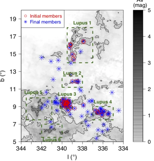
Figures 3 and4 show the proper motions, parallaxes and the colour-magnitude diagram of the Lupus stars selected in our membership analysis. The empirical isochrone that we derive from our membership analysis is given in TableA.3. Our sample of cluster members includes stars in the magnitude range from G '8 mag to G ' 18 mag. Most of the cluster members iden-tified in our study are located in Lupus 3 and 4 as illustrated in Fig. 5. We note that Lupus 1 and 2 host only a minor frac-tion of cluster members. Interestingly, our sample includes three and one stars projected towards Lupus 5 and 6, respectively. We confirm one star, namely Gaia DR2 6021420630046381440, from Manara et al. (2018) and another three stars (Gaia DR2 5995157042469914752, Gaia DR2 5997091667544824960 and GaiaDR2 5997086204346520448) fromMelton(2020) which are located in Lupus 5 and 6 as bona fide members of the region. We also confirm the existence of a more dispersed population of stars spread over the entire complex that is less numerous than the off-cloud population reported in pre-Gaia studies (see e.g.
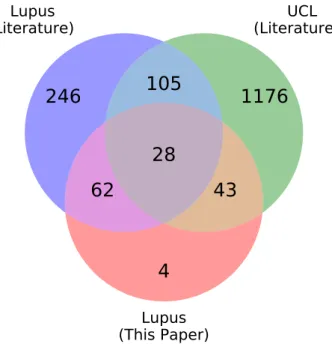
Krautter et al. 1997;Wichmann et al. 1997a,b;Galli et al. 2013). The Venn diagram represented in Fig.6shows that we have confirmed only 90 stars from previous studies as members of the Lupus association with our methodology. One important fraction of the literature sample with available data in Gaia-DR2, namely 351 stars, is rejected in our membership analysis.Damiani et al.
(2019) classified 105 of them as Sco-Cen members. Among the remaining 246 sources we verify that most of them (i.e. 148 stars) have small parallaxes ($ < 3 mas) confirming that they are indeed background stars unrelated to the Lupus region (as already anticipated in Sect. 2, see Fig. 2). We find more background sources at lower Galactic latitudes as also observed by Manara et al. (2018). The remaining sample of 98 sources
● ● ● ● ● ● ● ● ● ● ● ●● ● ● ● ● ● ● ● ● ● ● ● ● ● ● ● ● ● ● ● ● ● ● ● ● ● ● ● ● ● ● ● ● ● ● ● ● ● ● ● ● ● ● ● ● ● ● ● ● ● ● ● ● ● ● ● ● ● ● ● ● ● ● ● ● ● ● ● ● ● ● ● ● ● ● ● ● ● ● ● ● ● ● ● ● ● ● ● ● ● ● ● ● ● ● ● ● ● ●● ● ●● ● ● ● ● ● ● ● ● ● ●● ● ● ● ● ● ●● ● ● ● ● ● ● ● ● ● ● ● ● ● ● ● ● ● ● ● ● ● ● ● ● ● ● ● ● ● ● ● ● ● ● ● ● ● ● ● ● ● ● ● ● ● ● ● ● ● ● ● ● ● ● ● ● ● ● ● ● ● ● ● ● ● ● ● ● ● ● ● ● ● ● ● ● ● ● ● ● ● ● ● ●● ● ● ● ● ● ●● ● ●●●●●●●●●●●●●●●●●●●●●●●●●●●●●●●●●●●●●●●●●●●●●●●●●●●●●●●●●●●●●●●●●●●●●●●●●●●●●●●●●●●●●●●●●●●●●●●●●●●●●●●●●●●●●●●●●●●●●●●●●●●●●●●●●●●●●●●●●●●●●●●●●●●●●●●●●●●●●●●●●●●●●●●●●●●●●●●●●●●●●●●●●●●●●●●●●●●●●●●●●●●●●●●●●●●●●●●●●●●●●●●●●●●●●●●●●●●●●●●●●●●●●●●●●●●●●●●●●●●●●●●●●●●●●●●●●●●●●●●●●●●●●●●●●●●●●●●●●●●●●●●●●●●●●●●●●●●●●●●●●●●●●●●●●●●●●●●●●●●●●●●●●●●●●●●●●●●●●●●●●●●●●●●●●●●●●●●●●●●●●●●●●●●●●●●●●●●●●●●● AV = 1 mag 18 17 16 15 14 13 12 11 10 9 8 7 6 0.0 0.5 1.0 1.5 2.0 G−GRP (mag) GR P (mag) 0.80 0.85 0.90 0.95 Probability
Fig. 4.Colour-magnitude diagram of the sample of Lupus stars iden-tified in our membership analysis. The black solid line denotes the empirical isochrone of the Lupus association derived in this study (see TableA.3). The stars are colour-coded based on their member-ship probabilities which are scaled from zero to one. Triangles indicate the sources with RUWE ≥ 1.4 (see Sect.4.1). The arrow indicates the extinction vector of AV = 1 mag converted to the Gaia bands using the relative extinction values computed byWang & Chen(2019).
rejected from the literature includes 78 stars that are mostly spread well beyond the location of the Lupus clouds in a region not covered by our survey (l < 334◦) and exhibit different proper motions and parallaxes compared to the cluster members identi-fied in this paper. The other 20 stars are indeed projected towards the molecular clouds of the complex (mostly in Lupus 3), but only one of them, namely Gaia DR2 5997013327325390592, has proper motion and parallax consistent with membership in Lupus. This star has GRP= 11.77 mag and G − GRP= 1.65 mag
which puts it significantly above the empirical isochrone defined by the other cluster members (see e.g. Fig. 4). It was first
Fig. 5. Location of the Lupus stars overlaid on the extinction map of
Dobashi et al. (2005) in Galactic coordi-nates. Colours and symbols denote the initial list of candidate stars compiled from the literature (88 stars) and the final members identified from our membership analysis (137 stars). The rectangles indi-cate the position of the main molecular clouds defined byHara et al.(1999).
proposed to be a member of the Lupus association by
Damiani et al.(2019) and we found no more information about this star in the literature. We suspect that it is a binary or a high-order multiple system to explain its position in the colour-magnitude diagram.
A recent study conducted byTeixeira et al.(2020) and pub-lished during the revision process of this paper reports on the discovery of new YSOs with circumstellar discs in the Lupus complex. Two points are worth mentioning regarding the com-parison of our sample of cluster members with their results. First, the survey conducted by Teixeira et al. (2020) covers a larger area in the sky than our study and extends clearly beyond the location of the Lupus molecular clouds. They identified 60 new YSOs that are potential members of the Lupus complex (these sources are labelled as “Lupus and/or UCL” in Table 4 of that study), but only 39 of them are included in the field selected for our membership analysis in this paper. Second, the method-ology used in the two studies to select cluster members differs significantly.Teixeira et al.(2020) selected their sample of clus-ter members from proper motion cuts based on Lupus stars pre-viously identified in the literature. As shown in Fig. 6, many of the Lupus stars identified in the literature are probable field stars (unrelated to the Lupus clouds) and the adopted proper motion constraints in that study to select new members (i.e.
−27 < µαcos δ < 3 mas yr−1 and −33 < µδ < −13 mas yr−1) extend to a region in the proper motion vector diagram that is mostly populated by UCL stars (see Fig.2). As a result, we found only 3 stars (out of the sample of 39 sources) that are in com-mon with the study ofTeixeira et al.(2020). The remaining 36 sources listed byTeixeira et al.(2020) and included in our anal-ysis have mostly small membership probabilities suggesting that they are unrelated to Lupus. Indeed, the authors themselves con-cluded in their study that the older stars in the sample are most probably UCL members.
In this study, we report on the discovery of 47 new mem-bers of the Lupus association, which represents an increase of more than 50% with respect to the number of confirmed mem-bers already known from previous studies. Most of them (i.e. 43 stars) had previously been assigned to the Sco-Cen association byDamiani et al.(2019). One reason to explain this is that the authors included only Lupus 3 in their membership analysis so that the Lupus stars belonging to the other subgroups were either assigned to Sco-Cen or to the field population. The 43 stars pop-ulate all subgroups of the Lupus complex (except for Lupus 3) and our membership analysis focused on the properties of the whole region was able to identify them as members. In the fol-lowing we use our new sample of 137 members to revisit some properties of the Lupus star-forming region.
246
105
1176
4
62
28
43
Lupus
(Literature)
UCL
(Literature)
Lupus
(This Paper)
Fig. 6.Venn diagram comparing the number of Lupus stars compiled from the literature (with Gaia-DR2 data), Sco-Cen stars in the UCL subgroup, and the sample of confirmed Lupus members identified in this paper from our membership analysis.
4. Properties of the Lupus subgroups 4.1. Refining the sample of Lupus stars
We refine our list of cluster members by selecting the stars with the best astrometry in the sample to accurately determine the properties of the Lupus subgroups. We remove 24 stars with poor astrometric solution based the re-normalised unit weight error (RUWE) criterion2(i.e. with RUWE ≥ 1.4). These sources
exhibit the largest uncertainties in proper motions and parallaxes (see Fig.3) so that their membership status will require further investigation with future data releases of the Gaia space mission. This step reduces the sample of cluster members to 113 stars. 4.2. Proper motions and parallaxes
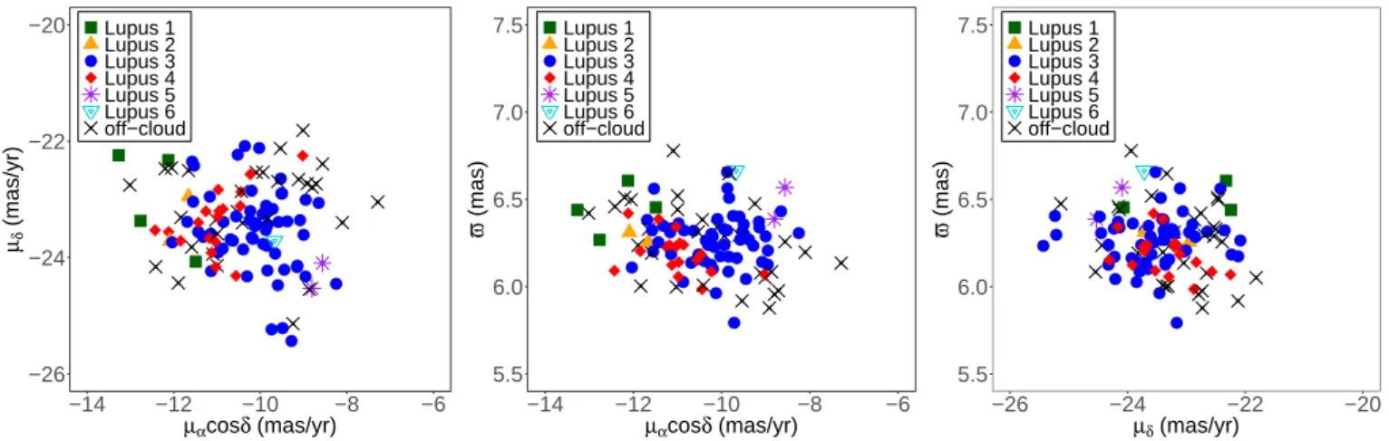
Figure 7 shows the distribution of proper motions and paral-laxes for the several subgroups of the Lupus complex. The mean values of each parameter are listed in Table 2. A first inspection of the sample reveals that the stars projected towards Lupus 3 exhibit different proper motions (in right ascension) that are shifted by about 1–2 mas yr−1 with respect to the stars in
Lupus 1, 2 and 4. This proper motion shift translates into 0.8– 1.5 km s−1in the tangential velocities of the subgroups. On the
other hand, we see no important differences between the proper motion components in declination and parallaxes among the var-ious subgroups of the Lupus complex.
We performed a two sample Kolmogorov-Smirnov test to quantitatively confirm our findings. We compare the distribution of proper motions and parallaxes from Lupus 3 stars with respect to the stars in the other molecular clouds (Lupus 1, 2 and 4). We find the p-values of 1.97 × 10⁻⁶, 0.64, and 0.23, for the analyses based on µαcos δ, µδand $, respectively. Thus, we conclude that
the proper motion component in right ascension is the most dis-tinctive astrometric feature that distinguishes the stars projected towards Lupus 3 from the other subgroups in the region. The few
2 See technical noteGAIA-C3-TN-LU-LL-124-01for more details.
stars in Lupus 5 and 6 that have been retained in our sample have proper motions that are more consistent with Lupus 3 stars.
This small difference in proper motions among the sub-groups is seen now for the first time with the more precise Gaia-DR2 data that is available nowadays. Previous studies about the kinematic properties of the Lupus region (see e.g.Makarov 2007; López Martí et al. 2011; Galli et al. 2013) used proper motions measured from the ground with a typical precision of about 2 mas yr−1that was not enough to detect subtle differences
of the stars located in different subgroups. The median uncertain-ties in proper motions and parallaxes for the Lupus stars in our sample based on Gaia-DR2 data are σµαcos δ = 0.15 mas yr−1,
σµδ = 0.09 mas yr
−1and σ
$= 0.08 mas, respectively. This
rep-resents an improvement in precision of about one order of mag-nitude with respect to pre-Gaia studies.
4.3. Radial velocities
We search for radial velocity information for the stars in our sam-ple using the CDS databases and data mining tools (Wenger et al. 2000). Our search in the literature is based onWichmann et al.
(1999), Gontcharov (2006), Torres et al. (2006), James et al.
(2006),Guenther et al. (2007), Galli et al.(2013), Frasca et al.
(2017), and the Gaia-DR2 catalogue. We find radial velocities for 52 stars in the sample of 113 sources with good astrome-try (see Sect.4.1). For a few stars we find more than one single radial velocity measurement and in such cases we use the most precise result.
The radial velocity distribution of the Lupus stars in our sam-ple is shown in Fig.8. We use the interquartile range (IQR) cri-terium to identify the outliers that lie over 1.5 × IQR below the first quartile or above the third quartile of the distribution. Only the radial velocity of Gaia DR2 5997015079686716672 satis-fies this condition. We discard this radial velocity measurement (Vr = 15.9 ± 0.7 km s−1,Frasca et al. 2017), but we still retain
the star in the sample because its proper motion and parallax are consistent with membership in Lupus.
We find that 20 candidate members in our sample of 113 stars have been identified as binaries or multiple systems in previ-ous studies (Ghez et al. 1997; Merín et al. 2008). Nineteen of them have radial velocity information in the literature, but only EX Lup (Gaia DR2 5996902860784332800) shows periodic radial velocity variations most probably due to a substellar com-panion (Kóspál et al. 2014). Analogously, we retain this star in the sample, but we do not use its radial velocity in the forthcom-ing analysis. Altogether, this reduces the sample of sources with radial velocity information to 50 stars.
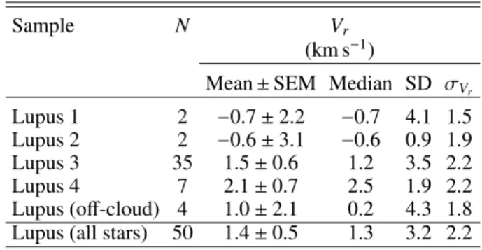
Table3 lists the mean radial velocity values for the Lupus subgroups (except for Lupus 5 and 6 which have no published data). We find no significant difference between the mean radial velocities of the subgroups within the uncertainties. The admit-tedly large scatter of radial velocities that is reported here is most probably related to the precision of the individual radial velocity measurements. The median uncertainty of the radial velocities in our sample is 2.2 km s−1. Removing the binaries
from the sample has negligible impact in reducing the radial velocity scatter. On the other hand, we note that the median uncertainty on the tangential velocities derived from Gaia-DR2 data is only 0.3 km s−1 and 0.4 km s−1 in the right ascension and declination components, respectively. Thus, the precision of the radial velocity measurements reported in the literature is currently the main limitation to investigate the dynamics (e.g. internal motions, expansion and rotation effects) of the Lupus complex.
● ● ● ● ● ● ● ● ● ● ● ● ● ● ● ● ● ● ● ● ● ● ● ● ● ● ● ● ● ● ● ● ● ● ● ● ● ● ● ● ● ● ● ● ● ● ● ● ● ● ● ● ● ● ● ● ● ● ● ● ● ● ● ● ●●● ● ● ● ● ● ● ● ● ● ● ● ● ● ● ● ● ● ● ● ● ● ● ● ● ● ● ● ● ● ● ● ● ● ● ● ● ● ● ● ● ● ● ● ● ● −26 −24 −22 −20 −14 −12 −10 −8 −6 µαcosδ (mas/yr) µδ (mas/yr) ● ● Lupus 1 Lupus 2 Lupus 3 Lupus 4 Lupus 5 Lupus 6 off−cloud ● ● ●● ● ● ● ● ● ● ● ● ● ● ● ● ● ● ● ● ● ● ● ● ● ● ● ● ● ● ● ● ● ● ● ● ● ● ● ● ● ● ● ● ● ● ● ●● ● ● ● ● ● ● ● ● ● ●● ● ● ● ● ● ● ● ● ● ● ● ● ● ● ● ● ● ● ● ● ● ● ● ● ● ● ● ● ● ● ● ● ● ● ● ● ● ● ● ● ●● ● ●● ● ● ● ●●● ● 5.5 6.0 6.5 7.0 7.5 −14 −12 −10 −8 −6 µαcosδ (mas/yr) ϖ (mas) ● ● Lupus 1 Lupus 2 Lupus 3 Lupus 4 Lupus 5 Lupus 6 off−cloud ● ● ● ● ● ● ● ● ● ● ● ● ● ● ● ● ● ● ● ● ● ● ● ● ● ● ● ● ●● ● ● ● ● ● ● ● ● ● ● ● ● ● ● ● ● ● ● ● ● ● ● ● ● ● ● ● ● ● ● ● ● ● ● ● ● ● ● ● ● ● ● ● ● ● ● ● ● ● ● ● ● ● ● ●● ● ● ●● ● ● ● ● ● ● ● ● ● ● ● ● ● ● ● ● ● ● ● ● ● ● 5.5 6.0 6.5 7.0 7.5 −26 −24 −22 −20 µδ (mas/yr) ϖ (mas) ● ● Lupus 1 Lupus 2 Lupus 3 Lupus 4 Lupus 5 Lupus 6 off−cloud
Fig. 7.Proper motions and parallaxes for the Lupus subgroups in our sample of cluster members. Table 2. Proper motions and parallaxes of the Lupus subgroups in our sample of cluster members.
Sample Ninit NRUWE µαcos δ µδ $
(mas yr−1) (mas yr−1) (mas)
Mean ± SEM Median SD Mean ± SEM Median SD Mean ± SEM Median SD Lupus 1 6 4 −12.414 ± 0.387 −12.446 0.773 −23.002 ± 0.439 −22.848 0.878 6.442 ± 0.069 6.447 0.139 Lupus 2 5 2 −11.875 ± 0.216 −11.875 0.433 −23.335 ± 0.383 −23.335 0.767 6.283 ± 0.028 6.283 0.056 Lupus 3 61 56 −10.118 ± 0.113 −9.986 0.843 −23.541 ± 0.095 −23.492 0.710 6.262 ± 0.020 6.272 0.148 Lupus 4 22 18 −10.997 ± 0.177 −11.006 0.753 −23.361 ± 0.125 −23.348 0.532 6.190 ± 0.027 6.194 0.116 Lupus 5 3 2 −8.684 ± 0.121 −8.684 0.241 −24.313 ± 0.217 −24.313 0.434 6.477 ± 0.091 6.477 0.182 Lupus 6 1 1 −9.669 ± 0.125 −9.669 −23.718 ± 0.094 −23.718 6.663 ± 0.053 6.663 Lupus (off-cloud) 39 30 −10.259 ± 0.263 −10.254 1.443 −23.162 ± 0.143 −22.954 0.782 6.256 ± 0.042 6.273 0.231 Lupus (all stars) 137 113 −10.378 ± 0.109 -10.306 1.155 −23.404 ± 0.068 −23.387 0.721 6.263 ± 0.017 6.265 0.178 Notes. We provide for each subgroup the initial number of stars, final number of stars after the RUWE filtering (see Sect.4.1), mean, standard error of the mean (SEM), median, and standard deviation (SD) of proper motions and parallaxes.
4.4. Distance and spatial velocity
In this section we re-visit the distance and kinematic proper-ties of the Lupus region based on our new sample of cluster members, the more precise Gaia-DR2 astrometry and the radial velocity measurements collected from the literature. The first step consists in correcting the Gaia-DR2 parallaxes by the zero-point shift of −0.030 mas that is present in the published data (see e.g.Lindegren et al. 2018). There are different estimates of the zero-point correction for the Gaia-DR2 parallaxes in the lit-erature that range from −0.031±0.011 mas (Graczyk et al. 2019) to −0.082 ± 0.033 mas (Stassun & Torres 2018), but we verified that the impact of this correction in our solution is negligible given the close proximity of the Lupus clouds. In addition, we also add 0.1 mas yr−1in quadrature to the formal uncertainties on the proper motions of the stars to take the systematics errors of the Gaia-DR2 catalogue into account (see e.g.Lindegren et al. 2018). This procedure is likely to overestimate the proper motion uncertainty for some stars in the sample given that the systematic errors in the Gaia-DR2 catalogue depend on the position, magni-tude and colour of each source (see e.g.Luri et al. 2018). These corrections are necessary for the purpose of estimating distances and spatial velocities with the corresponding uncertainties taking into account systematic errors, but they do not affect our results of the membership analysis.
Then, we used Bayesian inference to convert the observed parallaxes and proper motions into distances and 2D tangential
velocities. The prior that we used for the angular velocity (i.e. 2D tangential velocity) is a beta function following the online tuto-rials available in the Gaia archive (see e.g.Luri et al. 2018). We investigated two types of prior families for the distance. The first one is based on purely statistical probability density distributions (hereafter, statistical priors) and the second type is inspired on astrophysical assumptions (hereafter, astrophysical priors) e.g. the luminosity and density profiles of stellar clusters. The statis-tical priors investigated in this study are based on the Uniform and Gaussian distributions. The astrophysical priors include the surface brightness profile derived from star counts in the Large Magellanic Cloud byElson et al.(1987, hereafter, the EFF prior) and the King’s profile distribution derived from globular clusters (King 1962, hereafter, the King prior). We used the Kalkayotl code (Olivares 2019;Olivares et al. 2020)3 to compute the dis-tances with these different prior families. We refer the reader to that paper for more details on the properties, validation and per-formance of these priors. We are aware about the existence of another prior in the literature, namely the exponentially decreas-ing space density prior (hereafter, the EDSD prior,Bailer-Jones 2015;Astraatmadja & Bailer-Jones 2016), but we do not use it in our study. The EDSD prior is related to the distribution of stars in the Galaxy and it was proposed to be used in the context of large samples with wide distributions of parallaxes and uncertainties which is not the case of the Lupus sample.
3 The code is available at https://github.com/olivares-j/
−10 0 10 20 0.00 0.02 0.04 0.06 0.08 0.10 Radial Velocity (km/s) Density
before removing outliers after removing outliers
Fig. 8.Kernel density estimate of the distribution of radial velocity mea-surements for the sample of 52 members with available data. We used a kernel bandwidth of 2 km s−1. The tick marks in the horizontal axis mark the individual radial velocity values of each star.
Table 3. Radial velocity of the Lupus subgroups in our sample.
Sample N Vr
(km s−1)
Mean ± SEM Median SD σVr
Lupus 1 2 −0.7 ± 2.2 −0.7 4.1 1.5 Lupus 2 2 −0.6 ± 3.1 −0.6 0.9 1.9 Lupus 3 35 1.5 ± 0.6 1.2 3.5 2.2 Lupus 4 7 2.1 ± 0.7 2.5 1.9 2.2 Lupus (off-cloud) 4 1.0 ± 2.1 0.2 4.3 1.8 Lupus (all stars) 50 1.4 ± 0.5 1.3 3.2 2.2 Notes. We provide for each subgroup the initial number of stars, mean, standard error of the mean (SEM), median, standard deviation (SD) of the radial velocities, and the median uncertainty of the radial velocities.
We find no significant differences in the resulting distances obtained with different priors (Uniform, Gaussian, EFF and King) which agree within 1σ of the corresponding distance uncertainties. Thus, we confirm that our results are not affected by our choice of the prior. We have therefore decided to use the distances obtained with the Uniform prior, which is the sim-plest one, and report them as our final results. The distance and spatial velocity for individual stars in our sample are given in TableA.1together with other results derived in this paper. We use the resulting distances to compute the 3D position XYZ of the stars in a right-handed reference system that has its origin at the Sun, where X points to the Galactic centre, Y points in the direction of Galactic rotation, and Z points to the Galac-tic north pole. Then, we convert the 2D tangential velocity and radial velocity of the stars into the UVW Galactic velocity com-ponents in this same reference system following the transforma-tion outlined byJohnson & Soderblom(1987).
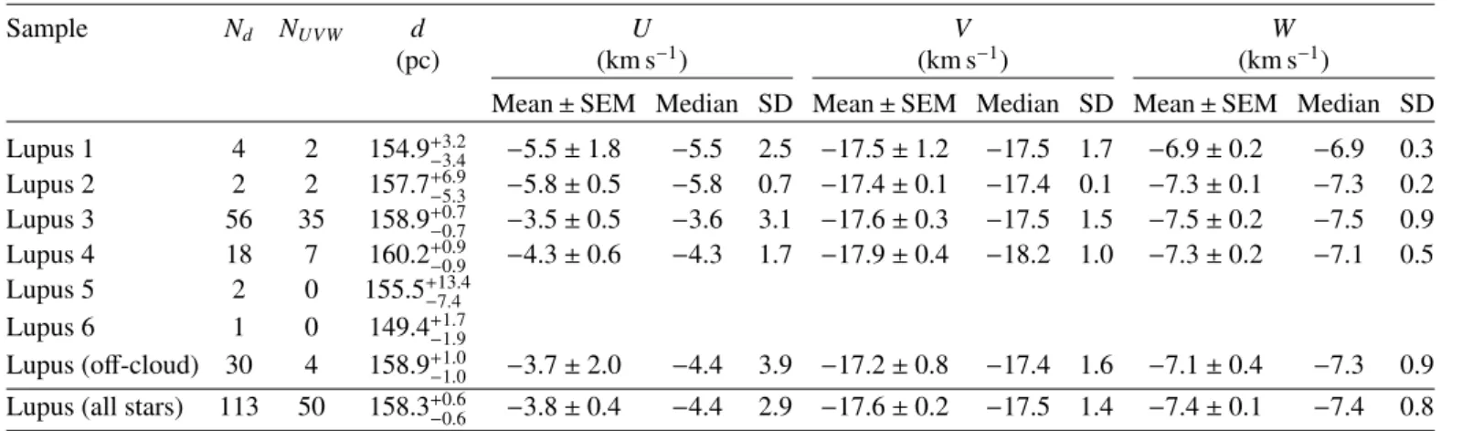
Table4 lists the distance and spatial velocity of the Lupus subgroups in our sample. The large uncertainties of our distance results observed for some subgroups can be explained by the small number of stars used in each solution. Our results reveal that the Lupus subgroups are located at the same distance (of about 160 pc) within the uncertainties derived for each solution. The only exception is Lupus 6 whose distance estimate given in Table4 is based on the parallax of one single star. Despite the common distance to the Sun, the subgroups (Lupus 1–4) are separated by about 8–20 pc among themselves in the space of 3D positions as illustrated in Fig.9.
The distances derived in this paper are still consistent with the results obtained by Dzib et al.(2018) despite the different samples of stars that have been used in each study. Our results do not confirm the large spread in distances of tens of par-sec along the line of sight reported in previous studies based on kinematic parallaxes (Makarov 2007;Galli et al. 2013) and
Hipparcos
data (see e.g.Bertout et al. 1999; Comerón 2008). One reason to explain the discrepancy with previous findings in the pre-Gaia era is the more precise and accurate data that is available nowadays to investigate the Lupus region. Another reason is the different samples of Lupus stars used in each study. For example, Makarov (2007) and Galli et al. (2013) included the more dispersed stars identified by Krautter et al.(1997) and Wichmann et al. (1997a,b) in their solutions (see Fig.1) which are mostly rejected in our membership analysis. In addition, many of the stars projected towards the molecular clouds and included in their analyses appear now to be back-ground sources unrelated to Lupus in light of the Gaia-DR2 data (see Sect.3).
The mean spatial velocities of the Lupus subgroups given in Table4confirm that they move at a common speed. We there-fore detect no significant relative motion between the subgroups at the level of a few km s−1 which is currently determined by
the precision of radial velocity data. The off-cloud population is located at the same distance and moves with the same velocity of the stars projected towards Lupus 1–4. This confirms that they are comoving with the on-cloud population and therefore belong to the same association.
We now compare the distance and kinematics of Lupus with the two adjacent subgroups of the Sco-Cen association (US and UCL). The relative motion of Lupus with respect to the space motion of US and UCL derived byWright & Mamajek(2018) is (∆U, ∆V, ∆W) = (2.4, −0.7, −0.4) ± (0.4, 0.2, 0.1) km s−1and (∆U, ∆V, ∆W) = (2.1, 2.4, −1.6) ± (0.4, 0.2, 0.1) km s−1,
respec-tively (in the sense Lupus “minus” US or UCL). This implies a relative bulk motion of 2.5 ± 0.4 km s−1 and 3.6 ± 0.3 km s−1
with respect to US and UCL, respectively.Damiani et al.(2019) revealed that Sco-Cen is made up of several substructures and the distances of the stars range from about 100 to 200 pc. The closest substructure of the Sco-Cen association to the Lupus molecular cloud complex is a compact group of 551 stars near V1062 Sco and named as UCL-1 (Röser et al. 2018;Damiani et al. 2019). The mean parallax of $ = 5.668 ± 0.011 mas and distance of 174.7+0.5−0.6pc put UCL-1 further away from the Sun as compared to Lupus (see Table4). Thus, despite the common location in the plane of the sky Lupus and Sco-Cen stars are located at different distances and exhibit distinct spatial velocities. Interestingly, we note that the observed difference between the spatial velocity of the Lupus clouds, UCL and US is comparable to the difference in spatial velocity of the Sco-Cen subgroups among themselves. The Lupus clouds could therefore be regarded as another sub-group of the Sco-Cen complex that resulted from a more recent star formation episode.
Table 4. Distance and spatial velocity of the Lupus subgroups in our sample of cluster members.
Sample Nd NUVW d U V W
(pc) (km s−1) (km s−1) (km s−1)
Mean ± SEM Median SD Mean ± SEM Median SD Mean ± SEM Median SD Lupus 1 4 2 154.9+3.2−3.4 −5.5 ± 1.8 −5.5 2.5 −17.5 ± 1.2 −17.5 1.7 −6.9 ± 0.2 −6.9 0.3 Lupus 2 2 2 157.7+6.9−5.3 −5.8 ± 0.5 −5.8 0.7 −17.4 ± 0.1 −17.4 0.1 −7.3 ± 0.1 −7.3 0.2 Lupus 3 56 35 158.9+0.7−0.7 −3.5 ± 0.5 −3.6 3.1 −17.6 ± 0.3 −17.5 1.5 −7.5 ± 0.2 −7.5 0.9 Lupus 4 18 7 160.2+0.9−0.9 −4.3 ± 0.6 −4.3 1.7 −17.9 ± 0.4 −18.2 1.0 −7.3 ± 0.2 −7.1 0.5 Lupus 5 2 0 155.5+13.4−7.4 Lupus 6 1 0 149.4+1.7−1.9 Lupus (off-cloud) 30 4 158.9+1.0−1.0 −3.7 ± 2.0 −4.4 3.9 −17.2 ± 0.8 −17.4 1.6 −7.1 ± 0.4 −7.3 0.9 Lupus (all stars) 113 50 158.3+0.6−0.6 −3.8 ± 0.4 −4.4 2.9 −17.6 ± 0.2 −17.5 1.4 −7.4 ± 0.1 −7.4 0.8 Notes. We provide for each subgroup the number of stars used to compute the distance (after the RUWE filtering) and spatial velocity, Bayesian distance, mean, standard error of the mean (SEM), median, and standard deviation (SD) of the UVW velocity components.
X (pc)
138140142144
146148150
65
60
55
Y (pc)
50
45
Z (pc)
0
10
20
30
40
Lupus 1
Lupus 2
Lupus 3
Lupus 4
Lupus 5
Lupus 6
off-cloud
Fig. 9.3D spatial distribution of the 113 members of the Lupus association. The different colours denote the various subgroups of the Lupus
star-forming region. The dashed lines connect each point in the plot to its projection on the XY plane (with Z= 0). The reference system used to represent the 3D spatial distribution of the stars is the same as described in the text of Sect.4.4.
4.5. Relative ages of the subgroups
In this section we compare the relative age of the subgroups based on the location of the stars in the HR-diagram compared to evolutionary models and the fraction of disc-bearing stars in each population. First, we use the Virtual Observatory SED Ana-lyzer (VOSA,Bayo et al. 2008) to fit the SED, derive the e ffec-tive temperatures and bolometric luminosities of the stars. We use the BT-Settl (Allard et al. 2012) grid of models to fit the SED and left the extinction AV as a free parameter (in the range
of 0–10 mag). We use the optical photometry from Gaia-DR2 and infrared photometry from the 2MASS (Cutri et al. 2003), AllWISE (Wright et al. 2010) and Spitzer c2d (Merín et al. 2008) surveys. We provide ourselves the photometric data of
the stars to the VOSA service when possible to avoid erro-neous cross-matches when querying these catalogues with the system interface. We cross-matched our sample of stars with the 2MASS and AllWISE catalogues using the source identi-fiers given in the auxiliary tables TMASS_BEST_NEIGHBOUR and ALLWISE_BEST_NEIGHBOUR available in the Gaia archive. We derived effective temperatures and bolometric luminosities for 110 stars in the sample with available photometric data. The two stars of Lupus 2 in our sample are among the three rejected sources with insufficient photometric data to fit the SED with VOSA.
We compare the effective temperatures obtained from the SED fits with those derived from the spectral type of the stars
● ● ● ● ● ● ● ● ● ● ● ● ● ● ● ● ● ● ● ● ● ● ● ● ● ● ● ● ● ● ● ● ● ● ● ● ● ● ● ● ● ● ●● ● ● ● ● ● ● ● ● ● ● ● ● ● ● ● ● ● ● ● ● ● ● ● ● ● ● ● ● ● ● ● ●● ● ● ● ● ● ● ● 1 Myr 5 Myr 10 Myr 100 Myr 0.02Μ0 0.03Μ0 0.05Μ0 0.1Μ0 0.3Μ0 0.5Μ0 1Μ0 1.4Μ0 −3 −2 −1 0 1 6000 5000 4000 3000 2000 Teff (K) log (L/ L0 ) ● ● Lupus 1 Lupus 3 Lupus 4 Lupus 5 Lupus 6 Lupus (off−cloud)
Baraffe et al.(2015) models
● ● ● ● ● ● ● ● ● ● ● ● ● ● ● ● ● ● ● ● ● ● ● ● ● ● ● ● ● ● ● ● ● ● ● ● ● ● ● ● ● ● ●● ● ● ● ● ● ● ● ● ● ● ● ● ● ● ● ● ● ● ● ● ● ● ● ● ● ● ● ● ● ● ● ●● ● ● ● ● ● ● ● 1 Myr 5 Myr 10 Myr 100 Myr 0.1Μ0 0.3Μ0 0.5Μ0 1Μ0 2Μ0 −3 −2 −1 0 1 6000 5000 4000 3000 2000 Teff (K) log (L/ L0 ) ● ● Lupus 1 Lupus 3 Lupus 4 Lupus 5 Lupus 6 Lupus (off−cloud)
Siess et al.(2000) models
Fig. 10.HR diagram of the Lupus star-forming region with theBaraffe et al.(2015) andSiess et al.(2000) evolutionary models. The solid and dashed lines represent isochrones and tracks, respectively, with the corresponding ages (in Myr) and masses (in M ) indicated in each panel. The most massive star in our sample (HR 5999) is not shown to improve the visibility of the low-mass range that includes the other stars in our sample. The error bars are smaller than the size of the symbols.
compiled from the literature (Hughes et al. 1994;Krautter et al. 1997; Comerón et al. 2009,2013; Alcalá et al. 2017). We find spectral classification for only 69 stars (i.e. 61% of the sample) and convert them to effective temperatures using the tables pro-vided byPecaut & Mamajek(2013). We observe a good agree-ment between the two effective temperature estimates with a mean deviation of −32 ± 31 K (in the sense, result from spec-tral type “minus” result from SED fit) and rms of 260 K. We have therefore decided to use the effective temperature estimates derived from the SED fits in the following analysis to work with a homogeneous data set and use this information for a more sig-nificant number of stars in the sample.
The resulting HR-diagram is shown in Fig.10. We compare the location of the stars in the HR-diagram with theBaraffe et al.
(2015) and Siess et al. (2000) models that combined together cover the entire mass range of our sample which ranges from about 0.03 to 2.4 M . Gaia DR2 5997082081177906048
(HR 5999) is a binary early-type star and the most massive mem-ber in our sample (m = 2.432 ± 0.122 M , see Vioque et al.
2018). The remaining sources in the sample are less massive than 1.4 M and fall into the mass domain covered by the
Baraffe et al.(2015) models. Our results suggest that the Lupus stars in the sample are mostly younger than 5 Myr. Many sources also lie above the 1 Myr isochrone and some of them are likely to be binaries or high-order multiple systems that will demand further investigation in future studies. Although age determi-nation at these early stages of stellar evolution is rather uncer-tain, we detect no evident age gradient or segregation among the Lupus subgroups from the HR-diagram analysis. TableA.4 pro-vides the age estimates inferred from the Baraffe et al. (2015) andSiess et al.(2000) models together with the results obtained from the SED fit with VOSA.
Alternatively, we compare the age of the subgroups based on the fraction of disc-bearing stars in each population. We compute
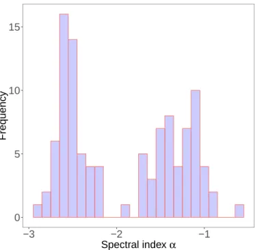
the spectral index α (Lada et al. 1987) of each source in the sam-ple with available photometric data in the infrared between 2 and 20 µm. This restricts the sample to 104 stars with AllWISE and Spitzerdata. Then, we classify the stars into Class I (embed-ded source, α > 0), Class II (disc-bearing star, −2 < α < 0) or Class III (optically thin or no disc, α < −2). We compare our results derived from the spectral index with the classifica-tion scheme proposed byKoenig & Leisawitz (2014) based on infrared colours and we obtain the same SED subclass for all stars in the sample.
Figure 11shows that the distribution of the spectral index α (see Table A.1) is bimodal suggesting the existence of two populations (disc-bearing and discless stars) with approximately the same number of sources. We verified that the bimodality of the distribution of spectral indices is not an artefact caused by the different number of points and wavelength range of the photometric data available for each star to compute the spectral indices. A similar result was also observed for the Chamaeleon I star-forming region (see Fig. 11 ofLuhman et al. 2008). Previ-ous studies suggested that the early disappearence of circumstel-lar discs could be related to environmental effects imposed by the presence of massive stars that produce strong UV radiation, stellar winds, and supernova explosions (see e.g. Walter et al. 1994; Martin et al. 1998). However, we see no dependency of the spectral index on the position of the stars in our sample and any nearby OB star surrounding the Lupus clouds to sup-port this scenario. As shown in Fig.10we note the existence of only a few stars older than 10 Myr in our sample which could be potential contaminants (as expected based on the performance of our classifier, see Table1). Thus, the hypothesis of contam-ination by older field stars does not explain the bimodality of spectral indices in our sample given that the two populations have the same number of stars, similar ages and are younger than the potential contaminants from the Sco-Cen association.