HAL Id: hal-01184338
https://hal.inria.fr/hal-01184338
Submitted on 14 Aug 2015
HAL is a multi-disciplinary open access
archive for the deposit and dissemination of
sci-entific research documents, whether they are
pub-lished or not. The documents may come from
teaching and research institutions in France or
abroad, or from public or private research centers.
L’archive ouverte pluridisciplinaire HAL, est
destinée au dépôt et à la diffusion de documents
scientifiques de niveau recherche, publiés ou non,
émanant des établissements d’enseignement et de
recherche français ou étrangers, des laboratoires
publics ou privés.
Hyperspectral Image Classification With Joint Spectral
and Spatial Information
Bharath Bhushan Damodaran, Rama Rao Nidamanuri, Yuliya Tarabalka
To cite this version:
Bharath Bhushan Damodaran, Rama Rao Nidamanuri, Yuliya Tarabalka. Dynamic Ensemble
Selec-tion Approach for Hyperspectral Image ClassificaSelec-tion With Joint Spectral and Spatial InformaSelec-tion.
IEEE Journal of Selected Topics in Applied Earth Observations and Remote Sensing, IEEE, 2015, 8
(6), pp.2405-2417. �10.1109/JSTARS.2015.2407493�. �hal-01184338�
Dynamic Ensemble Selection Approach
for Hyperspectral Image Classification
With Joint Spectral and Spatial Information
Bharath Bhushan Damodaran, Student Member, IEEE, Rama Rao Nidamanuri, Senior Member, IEEE,and Yuliya Tarabalka, Member, IEEE
Abstract—Accurate generation of a land cover map using
hyperspectral data is an important application of remote sensing. Multiple classifier system (MCS) is an effective tool for hyperspec-tral image classification. However, most of the research in MCS addressed the problem of classifier combination, while the poten-tial of selecting classifiers dynamically is least explored for hyper-spectral image classification. The goal of this paper is to assess the potential of dynamic classifier selection/dynamic ensemble selec-tion (DCS/DES) for classificaselec-tion of hyperspectral images, which consists in selecting the best (subset of) optimal classifier(s) rela-tive to each input pixel by exploiting the local information content of the image pixel. In order to have an accurate as well as com-putationally fast DCS/DES, we proposed a new DCS/DES frame-work based on extreme learning machine (ELM) regression and a new spectral–spatial classification model, which incorporates the spatial contextual information by using the Markov random field (MRF) with the proposed DES method. The proposed clas-sification framework can be considered as a unified model to exploit the full spectral and spatial information. Classification experiments carried out on two different airborne hyperspectral images demonstrate that the proposed method yields a significant increase in the accuracy when compared to the state-of-the-art approaches.
Index Terms—Dynamic classifier selection, dynamic ensemble
selection, hyperspectral image classification, markov random field model, multiple classifier system, spectral-spatial classification.
I. INTRODUCTION
H
YPERSPECTRAL image provides detailed spectral information in numerous narrow contiguous bands of the electromagnetic spectrum. This capability has led to the widespread use of hyperspectral images as an important data source for a range of applications, such as environmental monitoring, vegetation health monitoring, mineral exploration, military, and defence, etc. [1]–[3]. Supervised image classifi-cation has been extensively used to analyze hyperspectral data. However, several factors such as high dimensionality, spatialManuscript received September 04, 2014; revised February 06, 2015; accepted February 11, 2015. Date of publication March 25, 2015; date of current version July 30, 2015.
B. B. Damodaran and R. R. Nidamanuri are with the Department of Earth and Space Sciences, Indian Institute of Space Science and Technology, Thiruvananthapuram, Kerala 695 547, India (e-mail: bhushabhusha@ gmail.com; [email protected]).
Y. Tarabalka is with the INRIA Sophia Antipolis, 06902 Cedex, France (e-mail: [email protected]).
Color versions of one or more of the figures in this paper are available online at http://ieeexplore.ieee.org.
Digital Object Identifier 10.1109/JSTARS.2015.2407493
and spectral redundancy, interclass variability, noisy bands, and limited labeled samples make the information exploitation of hyperspectral images a very challenging task [4], [5]. Accurate hyperspectral image classification depends on the ability of the chosen classifiers to trade upon the relationship among available labeled samples, data dimensionality, and informa-tion classes. There is a high risk that the selected classifier is suboptimal for a problem and data at hand. Multiple classifier system (MCS) has been recently explored to improve the per-formance of hyperspectral image classification by combining the predictions of multiple classifiers [6]–[8], thereby reduc-ing the dependence on the performance of a sreduc-ingle classifier. For the MCS to perform better than the single best (SB) clas-sifier, the classifiers used in the MCS construction have to be diverse, because combining similar classification results may not improve accuracy [9].
Diversity in the MCS can be created explicitly and implic-itly. Explicitly, the diversity in the MCS is created by defining a diversity measure and optimizing it. Implicitly, diversity can be introduced by selecting a subset of features [10]–[12], train-ing samples manipulation, selecttrain-ing classifiers from different categories, and different feature extraction methods [13], [14]. However, the diversity constraint alone does not guarantee that the MCS always performs better. The possibility of inaccu-rate base classifiers and the incompatible combinations of the classifiers may instead end up the MCS with the suboptimal performance. An ensemble pruning approach has been pro-posed to select reasonably accurate base classifiers [15]–[17]. In this method, instead of combining all the available base clas-sifiers in the MCS, a subset of clasclas-sifiers is selected based on the criteria like diversity measures and performance measures for decision fusion. This approach has been expanded by propos-ing a unified framework [18] which consists of both diversity creation (implicit and explicit) and performance measures of base classifiers, as well as selecting the classifiers with nonzero weights by sparse optimization methods [19] to form an effec-tive MCS. However, the selection of classifiers in this method is independent of the location of the image pixel in the fea-ture space; hence, all the classifiers take part in classifying each image pixel. On the other hand, the optimal subset of classifiers varies for different spatial locations in the image. Therefore, the performance of the MCS can be improved by selecting the best classifier or a subset of classifiers dynamically relative to each image pixel, known as dynamic classifier/ensemble selection (DCS/DES) [20]–[22].
1939-1404 © 2015 IEEE. Personal use is permitted, but republication/redistribution requires IEEE permission. See http://www.ieee.org/publications_standards/publications/rights/index.html for more information.
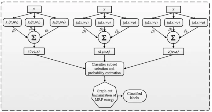
Fig. 1. Flowchart of the proposed spectral–spatial classification method.
The success of DCS depends on an accurate estimation of classifiers competence for a given image pixel. The classi-fiers forming a dynamic subset are chosen based on estimating the accuracy (competence) of each base classifier in a local region around the image pixel, and the selection is based on the highest accuracy criterion. The classifier competence can be computed by local accuracy (LA) estimation methods [22]– [24] and probabilistic model-based methods [25]. Recently, Du
et al. have studied the capability of DCS for hyperspectral image classification using LA estimation [26]. However, their study is limited with two optimal classifiers as the base clas-sifiers. When the number of base classifiers increases and in the presence of inaccurate classifiers, the performance of DCS based on LA is uncertain. Both the LA estimation methods and a probabilistic model approach compute the distance between the test pixel and the training (validation) samples. Hence, these techniques are computationally expensive for large-scale problems. The regression-based probabilistic model reduces the computational factor at the cost of the accuracy [25]. However, in practical situations, the accuracy is an important criterion in mapping applications. Recently, extreme learning machine (ELM) has shown good performance in terms of both compu-tational time and accuracy for the classification and regression problems [27]. In this paper, we modeled the DCS problem as the classification problem by mapping the validation samples to the classifier competence measure based on ELM regres-sion. The proposed DCS/DES method based on ELM increases the efficiency in computation time and classification accuracy for the large-scale problems. Our extensive literature review reveals that the potential of the DCS/DES approaches for the hyperspectral image classification is not well studied. Hence, it is highly desirable to study the potential of the DCS/DES approaches, and develop an accurate and computationally efficient DCS/DES methodology for hyperspectral image classification.
Apart from the spectral content, airborne hyperspectral sen-sors also provide rich spatial information, which has been extensively utilized in recent studies for hyperspectral image classification [28]–[30]. Markov random field (MRF) model is a powerful method for modeling the spatial contextual infor-mation, which assumes that the neighboring pixels are likely to belong to the same class [31]–[33]. Most of the state-of-the-art
studies deal with MRF regularization for a single classifier, yielding significant improvement in the classification perfor-mance [32], [34], [35]. The perforperfor-mance of MRF regularization depends on the accuracy of the classifier’s probability esti-mates. It has been shown that the combination of several classifiers yields reliable probability estimates when compared to the single classifier. Thus, the use of an MCS to derive the data energy term for the MRF regularization is likely to improve the classification accuracy. However, only few stud-ies tested the application of an MRF model to the MCS-based image classification [36], [37]. Furthermore, DCS/DES over-comes the structural limitation of a single classifier, as well as classifier combination or classifier fusion (CF) methods and provides more reliable probability estimates. Thus, DCS/DES emerges as a strong candidate to capture the spectral informa-tion of a hyperspectral image. There are no studies available in literature which test the application of an MRF model to the DES based image classification. Hence, the combi-nation of the DES to extract spectral information with the MRF model to exploit spatial context into a unified frame-work would yield a powerful tool for hyperspectral image classification.
The main contributions of this paper are as follows. 1) We tested the performance of different DCS and DES methods, and compared the performance between DCS and DES methods for hyperspectral image classification. 2) We propose an extended version of the probabilistic model-based DES based on ELM approach. 3) We propose a new unified framework to exploit both spectral and spatial information based on DES and MRF models for hyperspectral image classification.
The flowchart of the proposed spectral–spatial DES method is shown in Fig. 1. This framework extracts the spectral infor-mation by using the DES method and the spatial inforinfor-mation by applying the MRF model. Experiments had been conducted with two multisite airborne hyperspectral images, and results showed that proposed method yielded the improved classifi-cation accuracies when compared to the previously proposed techniques.
The remainder of this paper is organized as follows. Section II gives an overall view of the DCS and the proposed approaches. In Section III, we report the experimental results and we discuss and conclude them in Section IV.
II. METHODOLOGY
In this section, we first describe about different DCS/DES methods which we propose to apply for hyperspectral image classification and later these methods are used for compari-son with our proposed method. Then, we present the proposed DCS/DES-ELM method and spectral–spatial DES approach. The term DCS indicates that only the best classifier is selected relative to each image pixel, whereas DES indicates that the subset of best classifiers is selected relative to each image pixel.
A. MCS
Let Ψ = {ψ1, ψ2, . . . , ψL} be the base classifiers forming an MCS, and each classifier ψl, l = 1, 2, . . . , L be a function ψl: χ→ Ω from an input space χ ⊆ Rnto a set of class labels Ω ={ω1, ω2, . . . , ωM} (M is the number of classes). For any given x ∈ χ, a classifier ψlproduces a vector of decision values d = [dl1, dl2, . . . , dlM] and x is assigned to the class that has the maximum probability (decision) value. The base classifiers have to commit different types of errors in their predications on different parts of the input space, so that the MCS produces more accurate results when compared to individual classifiers. The random subspace method (RSM) is a popular ensemble generation technique to generate multiple input data sources from a single input data, thus creating diversity among the classifiers in an MCS [12].
The RSM partitions hyperspectral image bands into L sub-sets and each subset contains P
L number of bands, where P denotes the number of bands in the original hyperspec-tral image. Each input data source generated from the RSM is returned as the input to the learning algorithm ψ. Support vector machines (SVM) have gained interest in hyperspectral image classification due to their ability to deal effectively with high-dimensional data and small training sets [38], [39]. The performance of SVM varies across different input data sources, thus introducing diversity in the MCS. Apart from SVM, RSM also has the capability to mitigate the small sample size problem and offers good classification accuracies in the heterogeneous environment. The SVM coupled with the output from the RSM were used as base classifiers in the MCS. The concept of com-bining all the base classifiers available in the MCS to obtain the final classified image, known as classifier combination or CF method, was extensively explored. Therefore, here we focus on the DCS/DES approach, which dynamically selects the best (subset of) classifier(s) for a given image pixel. In the following section, we describe the various dynamic classifier approaches that we propose to apply for hyperspectral image classification.
B. DCS and DES Approaches
The basic idea of the DCS is to find the classifier with the highest probability of being correct for a given unseen sample. The selection of correct classifiers and hence the suc-cess of the DCS depends on the estimation of the classifiers competence for a given sample. The classifier competence measure is estimated from validation samples (different from training samples and test samples). Apart from the train-ing and test samples, validation samples are also generated
for estimating the classifier competence in DCS. Let V = {(v1, j1) , (v2, j2) , . . . , (vN, jN)} be the validation set con-taining pairs of validation samples and their corresponding class labels. A brief description of different methods used to estimate the classifier competence is given below.
1) DCS/DES by LA Estimate (DCS/DES-LA): The DCS/DES-LA estimates accuracy of each classifier in a local surrounding region of the image pixel and selects the classifier that exhibits higher LA [23]. Let x be an image pixel to be classified and let us consider k-nearest neighbors of x in the validation set, denoted as Q (x) ∈ V . Without loss of generality, we assume that the classifier ψlassigns a class label ωm to the image pixel x (i.e., ψl(x) = ωm). Then, the LA of a classifier ψl (LA is known as the classifier competence measure) is denoted by LA (ψl|x) = Nm !M i=1Nim , Q (x)∈ V |ψl(vj) = ωm, j = 1, 2, . . . , k (1)
where Nmis the number of correctly classified samples by the classifier ψl to the class ωmin the neighborhood Q (x) ,and !M
i=1Nim is the number of the k-nearest samples of x in V that have been assigned to the class ωm by the classifier ψl. The classifier which exhibits the highest LA is selected as the adaptive classifier for image pixel x:
l = arg maxiLA (ψi, x) . (2) However, in this approach, all the neighboring samples are given equal significance and probability values of the classifiers have not been considered. The validation samples that are closer to the image pixel may have more impact than the samples that are farther away. The classifiers probability values are weighted based on the distance to the neighboring samples, to improve the estimation of LA [22], labeled as posterior LA (PLA). The PLA is estimated as P LA (ψl, x) = ! vj∈ωmP (ωm|vj, ψl) wj !M i=1 ! vj∈ωiP (ωm|vj, ψl)wj , Q (x)∈ V |ψl(vj) = ωm (3) where vj∈ Q (x) , P (ωm|vj, ψl) is the posterior probability value of the validation sample vj assigned to the class ωm by the classifier ψl and wj= 1/dj, dj is the Euclidean dis-tance between the image pixels x and vj. The classifier that has the maximum PLA is selected for classifying the image pixel x similar to (2). In order to select a subset of T classi-fiers, the classifier competence values (PLA, LA) are arranged in descending order and the first T classifiers are selected. The classification process is then performed by using weighted Bayesian average methods [40] and is called DES
P (ωi/x) = "T
t=1ηtpt(ωi/x) , i = 1, 2, . . . , M. (4) The class label is obtained as x ∈ ωm, m = arg maxi P (ωi/x), where ηt is the weight of the classifier ψt [for instance, it is obtained as ηt= P LA (ψt, x)], and pt(ωi/x) is the resulting posterior probability of class ωifor a classifier ψt.
2) DCS/DES With Modified LA (DCS/DES-MLA): This approach is similar to DCS/DES-LA, except that the LA is esti-mated using weighted nearest neighbors of the image pixel x. Motivated by the performance of the distance weighted k-NN classifier, Smits [24] used generalized Dudani’s weighting scheme for scaling distance with the sth nearest neighbor for scaling the distances as
wr(x) = ⎧ ⎨ ⎩ dk− dr ds− d1 ds̸= d1, s = 3k 1, otherwise (5) where dk is the distance between kth sample and the image pixel x, and dris the distance between the rth of the kth nearest neighbor and the image pixel x. The MLA is then estimated as
M LA (ψl, x) = 1 k " j∈N(x)|ψl(x)=ωm wj. (6) The classifier which exhibits the maximum LA is cho-sen to classify each image pixel. If a subset of classifiers is selected, then classification is performed similar to (4) with ηt= M LA (ψt, x). Furthermore, we modified (6) by incorpo-rating classifiers posterior probability values of the neighboring samples for better LA estimation
M P LA (ψl, x) = ! vj∈ωmp (ωm|vj, ψl) .wj !M i=1 ! vj∈ωip(ωm|vj, ψl).wj , Q (x)∈ V |ψl(vj) = ωm (7) where wj is the weight obtained from (5), and p (ωm|vj, ψl) is the posterior probability value of the validation sample vj assigned to the class ωm.
3) DCS/DES-Beta Probabilistic Model (DCS/DES-Beta):
The third employed method to estimate the classifier com-petence is based on the beta probabilistic model [25]. The classifier competence is modeled as the probability of correct classification of a random reference classifier (RRC). The RRC produces a randomized vector of class supports, such that its expected value is equal to the vector of class supports produced by the classifier ψlfor each of the samples vj, j = 1, 2, . . . , N in the validation set. The RRC depends on the beta probability distribution with the parameters αm,βm, m = 1, . . . , M . The parameters αmand βm are derived from the vector of class supports produced by the classifier ψl.
Let ωj be an original class label of the sample vj∈ V , and the classifier ψl produces a vector of class supports as [d1(vj), d2(vj), . . . , dM(vj)]. The estimation of classifier competence can be summarized as
1) estimate the parameters of beta distribution as αm= M dm(vj), βm= M [1− dm(vj)];
2) construct the RRC and compute its conditional probabil-ity of correct classification as
Pc(RRC|vj) = & 1 0 b(u, αmj(vj), βmj(vj)) '(M m=1,m̸=ωj B (u, αm(vj), βm(vj)) ) du (8)
where b (u, αmj(vj), βmj(vj)) is the beta probability dis-tribution and B (u, αm(vj), βm(vj)) =∫0ub (w, αm(vj), βm(vj)) dw is the beta cumulative distribution function. The classifier competence (C) for each validation sample is estimated as
C (ψl, vj) = Pc(RRC|vj), j = 1, 2, . . . , N ;
l = 1, 2, . . . , L. (9)
The classifier competence is computed for all the validation samples, which essentially indicates which classifier is most suited for the validation samples. In order to choose the opti-mal classifier for a given image pixel, the classifier competence set is generalized to the entire feature space as follows:
c (ψl, x) = !N j=1C (ψl, vj) exp * −dist(x, vj)2 + !N j=1exp * −dist(x, vj)2 + (10)
where dist is the Euclidean distance between the image pixel x and the validation samples. The most competing classifier is selected for each pixel similar to (2). If the subset of competent classifiers is selected, then image pixels are classified by using (4). Criterion (10) is known as potential model (DCS/DES-beta potential). This method eliminates the necessity of finding the nearest neighbors for each image pixel x; instead, it weights the validation samples that are closer to x with high weights and the validation samples that are farther away with low weights. However, it is required to compute N distances for each image pixel, yielding high computational complexity, especially when the image size is large.
In order to reduce the computational complexity, the clas-sifier selection problem can be formulated as the regression problem. Let us consider L classifiers as L classes; the objec-tive is to learn a function that selects a classifier for each of the image pixels. In other words, the classifier selector is a func-tion f: V → C that maps from the validafunc-tion data set to the competence set of validation samples.
Let {(v1, C (ψl, v1)), . . . , (vj, C (ψl, vj))} , l = 1, . . . , L be pairs of a validation sample and its corresponding classifier competence value of the classifier ψl. For simplicity, let C (ψl) = [C (ψl, v1) , C (ψl, v2) , . . . , C (ψl, vN)], now
f (V ; βl) = βltV ⇒ βltV = C (ψl) (11) where βl is the parameter to be estimated for the classifier ψl. The classifier competence of the image pixel x can be obtained by
c (ψl, x) = βltφ (x) (12) and the parameter βlcan be obtained by pseudoinverse as
βl= ,
ΦtΦ-−1ΦtC (ψ
l) (13)
where Φ = [φ (v1), . . . , φ (vn)] and φ (v) is the polynomial transformation of the sample v as !r
i=0vi, r = 2, 3, 5. We empirically set r = 3. The classifier that has the maximum competence value in (12) is selected to classify the image pixel
Fig. 2. Flowchart of the proposed DCS/DES-ELM and DES-ELM + MRF method.
x. We call this method as the DCS-beta least square regression (DCS-beta-LSR). When a subset of classifiers is considered, then the classification is performed by applying (4), and we call it DES-beta-LSR.
C. Proposed DCS/DES-ELM Method and Spectral–Spatial DES Approach (DES-ELM + MRF )
In this section, we propose an extended version of the probabilistic model-based DCS/DES based on ELM approach. Furthermore, this proposed method is regularized with MRF model to develop spectral–spatial DES approach for hyper-spectral image classification. The flowchart of the proposed DCS/DES-ELM and spectral-spatial DES is shown in Fig. 2
The performance of the DCS/DES-beta-LSR depends on the feature transformation of the validation and input samples. It has been shown that the DCS/DES-beta-LSR has a suboptimal performance compared to the DCS/DES-beta potential model [25]. Hence, it would be beneficial to have a DCS/DES approach which is independent of feature transformation. Recently, ELM has demonstrated its superior capability to offer better generalization ability and fast training speed for classification and regression problems [27], [41], [42]. In this paper, we propose DCS/DES based on ELM for accurate and fast hyperspectral image classification, labeled as DCS/DES-ELM. The ELM method has the inherent ability to transform the input samples. In addition to that, the performance of the ELM is independent of its parameters, and a wide variety of transformation functions can be used.
The DCS/DES-ELM approach can be modeled as "R
i=1βigi(wi, vj) = C (ψl, vj)⇒ h (vj) β = C (ψl, vj) ,
j = 1, 2, . . . , N (14)
where R is number of the hidden nodes, h (vj) = [g1(w1, vj) , . . . , gR(wR, vj)] is the output row vector of hidden layer for input vj, gi(wi, vj) is the output of the transformation function in the ith hidden node [radial basis function (RBF) is used as the transformation function, and the input weights wiare ran-domly chosen], β = [β1, . . . , βR]tis the output weight between the hidden layer nodes and the output nodes, and C (ψl, vj) is competence value of the jth validation sample of the classifier ψlobtained from (9).
For all the validation samples j, (14) can represented as
Hβl= C (ψl) (15) where H = ⎡ ⎢ ⎣ h (v1) .. . h (vN) ⎤ ⎥
⎦, the parameter βl is the weight vec-tor of the hidden layer matrix and classifier competence value of the validation samples for the classifier ψl, and this can be obtained as
βl=,HtH-−1HtC (ψl) . (16) The classifier competence for an image pixel x is com-puted as
c (ψl, x) =,HtH-−1HtC (ψl) h (x) . (17) The competence values are arranged in the descending order and the first T classifiers are selected as adaptive classifiers for the image pixel x. Then, classification is performed by com-puting the weighted Bayesian average (4), with ηt= c (ψt, x), and we call it as DES-ELM. The class label is obtained as x∈ ωm, m = arg maxiP (ωi/x) (Fig. 2).
Spectral–Spatial DES approach: In the proposed method, the spatial contextual information is incorporated into the
DES-ELM classification by using the MRF-based regulariza-tion model. The DES method is only regularized with MRF model, as the DES method provides better class posterior prob-ability estimates than the DCS method. In the MRF framework, the classification task is formulated as an energy minimization problem on the graph of image pixels. The energy to opti-mize is computed as a sum of spectral and spatial energy terms and assumes that a pixel belonging to a specific class tends to have neighboring pixels belonging to the same class. The MRF model can be written as
ˆ ω = arg minω * −"i ∈Slog P (ωi/xi) + γ" j∈N(xi) (1− δ(ωi, ωj)) 4 (18) where δ (·) is the Kronecker function [δ (ωi, ωj) = 1 for ωi= ωj; δ (ωi, ωj) = 0 for ωi̸= ωj], N (xi) is the neighboring pix-els of xi, ˆω is the resulting class labels from the MRF regularization, S is the set of all image pixels, and γ is a pos-itive constant parameter that controls the importance of spatial smoothing. The first term P (ωi/xi) characterizes the spectral information and it is derived from the DES-ELM by employ-ing (4). The second term is expressed by usemploy-ing a Potts model, which favors spatially adjacent pixels to belong to the same land cover class [43]. This MRF regularization is solved by applying an efficient α-expansion graph-cut-based algorithm described in [44].
III. EXPERIMENTALRESULTS
A. Hyperspectral Image Description
In order to study the potential of DCS/DES for hyperspectral image classification, we adopted two benchmark hyperspec-tral images with different land cover settings (one in the urban area and one in the agricultural area) captured by two different sensors (ROSIS and AVIRIS).
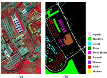
ROSIS University: The first hyperspectral data set was col-lected over the University of Pavia, Italy by the ROSIS airborne hyperspectral sensor in the framework of HySens project man-aged by DLR (German national aerospace agency). The ROSIS sensor collects images in 115 spectral bands in the spec-tral range from 0.43 to 0.86 µm with a spatial resolution of 1.3 m/pixel. After the removal of noisy bands, 103 bands were selected for experiments. The image contains 610 × 340 pixels with nine classes of interest. Fig. 3 shows a false color compos-ite (FCC) image and its corresponding ground truth map.
AVIRIS Indian Pines:The second hyperspectral image was collected by the AVIRIS sensor over the Indian Pines site in the Northwestern Indiana. The AVIRIS sensor collects images in 220 spectral bands in the spectral range from 0.43 to 0.86 µm at 20-m spatial resolution. Twenty water absorption bands were removed, and 200 bands were used for experiments. This image contains 145 × 145 pixels with 16 classes of interest. Fig. 4 shows the FCC image and its corresponding ground truth map.
Fig. 3. (a) FCC of the ROSIS University image (R: 0.8340 µm G: 0.6500 µm B: 0.5500 µm). (b) Ground truth image and its corresponding class labels.
B. Design of Experiments
From the available ground truth samples, we randomly selected 100 samples for training, 100 samples for validation, and the remaining samples were used for testing (see Tables I and II). If the total number of available reference samples was lower than 300 samples per class, then 25% of samples were selected for training, another 25% of samples for validation, and remaining samples were used as the testing samples. The exper-imental results were assessed by overall accuracy (OA), average accuracy (AA), and producer accuracy (PA). In order to avoid the bias induced by random sampling of the training and valida-tion samples, ten independent Monte Carlo runs are performed and the accuracies (OA, AA, PA) are averaged over the ten runs. In each of the RSM, multiclass pair-wise probabilistic SVM classification with the Gaussian RBF kernel was performed [44]. The SVM parameters in all experiments were automat-ically tuned by using fivefold cross-validation with C = 2α, α ={−5, −4, . . . , 15} and γ = 2β, β ={−15, −13, . . . , 3} (C is the cost function and γ is the width of the RBF kernel). When using the DCS-LA and DCS-MLA methods, the classi-fier competence was estimated based on both strategies (1) and (3), and the best results were retained. The performance of the DCS-LA and DCS-MLA approaches depends on the k-nearest neighbors of the test sample in the validation data set. Hence, we varied the value of k from 3 to 25 and only the best classifi-cation accuracies were retained. When more than one classifier was selected, the performance of the DES depended on the number of classifiers (T ) included in (4). Hence, in the exper-iment, we varied the number of classifiers from 2 to 7 and only the best accuracy is reported. However, in most of the Monte Carlo runs, the optimal results were obtained with four and five classifiers. The parameters of ELM regression were automati-cally tuned using fivefold cross-validation method. In the MRF model (18), the parameter γ that controls the spatial smoothness was tuned empirically for the optimal classification results.
Furthermore, the classifier combination or CF method using Bayesian average algorithm was adapted to combine all the
Fig. 4. (a) FCC of the AVIRIS Indian Pines image (R: 0.8314 µm G: 0.6566 µm B: 0.5574 µm). (b) Ground truth image and its corresponding class labels.
base classifiers in the MCS [40] to compare with the DCS/DES-ELM approaches. The results of the proposed spectral–spatial DES (DES-ELM + MRF) were compared with the results of the full-band SVM classification, full-band ELM classification, SB classifier, and CF. Apart from this, the proposed spectral– spatial DES method was compared with the four state-of-the art approaches, full-band SVM + MRF [32], full-band ELM + MRF, MCS + MRF [36], composite kernels (CK) [30], and SVM ensemble fusion [12]. In the CK [30], the spatial and spectral kernels are combined to exploit the spectral and spatial information of the hyperspectral image. The spatial component of the kernel was derived from the mean of the spectral bands over a spatial neighborhood. The spectral component of the kernel was derived from the spectral information of the indi-vidual pixels. The Gaussian RBF and the polynomial kernel were considered in the CK. The experiments were conducted with different combination of the kernels (for instance, polyno-mial kernel for spectral information and RBF kernel for spatial information), and only the best accuracies were reported (for both images, RBF kernel was used for both spectral and spatial information). We tuned hyperparameters of the composite ker-nel γ, and C by using fivefold cross-validation and we varied the parameter µ between 0 and 1.
In the SVM ensemble fusion method [12], the hyperspec-tral image was partitioned into different subsets (i.e., 4 and 6 subsets for the ROSIS University and AVIRIS Indiana Pines hyperspectral images) using correlation coefficient, and each of these subsets was classified by SVM classifier. The decision function values of the individual SVM classifier were fused by one more SVM classifier (the hyperparameters are optimally tuned by fivefold cross-validation). The same number of train-ing and testtrain-ing samples were used for computtrain-ing the accuracy of the state-of-the art approaches.
C. Classification Results of RSM
Table III shows the classification accuracies of SVM clas-sification relative to each random subspace. The results show that there is a considerable variability among the base classi-fiers in the MCS in terms of OA and class-specific accuracies, thus indicating the suitability of RSM for forming the MCS. The variability of classifiers accuracy is less significant for the University image. There is a 2% accuracy difference between the maximum and minimum overall classification accuracy in the MCS, whereas it is about 8% difference for the AVIRIS Indian Pines hyperspectral image.
TABLE I
NUMBER OFREFERENCESAMPLESCONSIDERED FOR THEEXPERIMENT OFUNIVERSITYIMAGE
D. Classification Results of the DCS and DES
In this section, the classification results of the differ-ent DCS/DES approaches and the proposed DES-ELM, DES-ELM + MRF methods are presented. Tables IV and V summarize accuracies of the DCS/DES for both hyperspectral images. DCS indicates that only the most competent classifier is selected for each image pixel, whereas DES indicates that a sub-set of classifiers was selected for each image pixel. The DCS, DCS-LA, and DCS-ELM methods yield a marginal increase in overall classification accuracies. The remaining methods resulted in 2% decrease in classification accuracies when com-pared to the SB classifier for both images. This observation highlights the need to select an adaptive subset of classifiers for each image pixel, instead of choosing only the most competent classifier. This is analogous to the case of selecting multiple classifiers instead of one classifier to avoid the risk of the suboptimal performance.
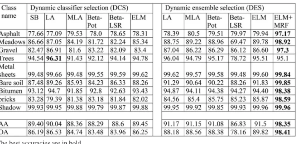
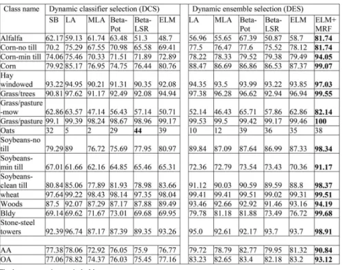
When a subset of classifiers is chosen for each image pixel and combined by the weighted Bayesian average method, the classification accuracy is significantly improved with all the DES approaches (except the DES-LSR method for the University image). There is a significant improvement in classification accuracy (about 5–6 percentage points) for the Indian Pines image, and a moderate improvement (about 2–3 percentage points) for the University image. Among the DES approaches, the DES-ELM achieved the highest accuracy for the University image and the DES-LA, DES-potential, and DES-ELM achieved the highest accuracies for the Indian Pines image.
The per-class and average-class accuracies have also been improved. There is about 7%–8% improvement in per-class
TABLE II
NUMBER OFREFERENCESAMPLESCONSIDERED FOR THEINDIANPINESIMAGE
TABLE III
OAANDAA (INPERCENTAGE)OF THESVM CLASSIFICATIONRELATIVE TOEACH
RANDOMSUBSPACE ANDFULL-BANDHYPERSPECTRALIMAGE
TABLE IV
PA, OA,ANDAA (INPERCENTAGE)OF THEDCSANDDES METHODS FOR THEUNIVERSITYIMAGE
The best accuracies are in bold.
accuracy for most of the classes in the Indians Pines image, while it is moderate with the University image. This observa-tion supports the need of adopting the adaptive classifiers based on local pixel information for enhanced classification perfor-mance. However, the poor per-class accuracy is observed with the classes oats and alfalfa. This is because the classifier fails to characterize the class information due to the presence of the insufficient number of training samples. Furthermore, our proposed DES-ELM approach has outperformed other DES methods in terms of both accuracies and computational time (see Table VI).
From the above observations, we can conclude that DES-ELM better characterizes the spectral information and provides reliable probability estimates and class labels when compared to the other considered methods. The inclusion of spatial con-textual information in DES-ELM by the MRF model further significantly increases classification performance. In this case (DES-ELM + MRF), the overall and average classification
accuracies are improved by 12%–15% and by 9%–12% over the SB classifier, respectively. When compared to its earlier ver-sion (DES-ELM), about 9% enhancement in the classification accuracy is observed. Furthermore, the class-specific accuracies exceed 95% for medium and large spatial structures, and are less than 95% for small spatial structures (e.g., trees, alfalfa,
and oats). The lower per-class classification accuracy of oats
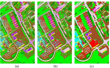
and alfalfa might be due to insufficient number of training samples. The classification maps of the SB, DES-ELM, and DES-ELM + MRF are shown in Figs. 5 and 6. Visual inspec-tion of Figs. 5(a) and (b), and 6(a) and (b) reveal that DES produced smoother classification maps than the SB classifier. Figs. 5(c) and 6(c) confirm a significant increase in classifica-tion accuracies and highlight the potential of the MRF model to produce a smooth classification map with spatially connected regions.
Computational time analysis: Table VI shows the com-putational time of the different DES approaches for both
TABLE V
PA, OA,ANDAA (INPERCENTAGE)OF THEDCSANDDES METHODS FOR THEINDIANPINESIMAGE
The best accuracies are in bold. TABLE VI
CPU PROCESSINGTIME(INSECONDS)OF THEDIFFERENT
DES APPROACHES
Since the RSM generation includes for all the methods, the CPU processing time of RSM generation is discarded.
hyperspectral images. The computational time complexity of the DES-LA, DES-MLA, and DES beta potential methods is very high and it grows with the number of pixels to be classified, thus impeding the use of the DES approaches for the large-scale image classification. On the other hand, the DES-LSR and DES-ELM methods are independent of the number of pixels in the image and thus perform very fast image classification. It can be seen from Tables IV to VI that the proposed DES-ELM method outperforms the other DCS/DES approaches in terms of accuracy and computational time.
E. Comparative Performance of the Proposed Methods With the State-of-the Art Approaches
The accuracy of the DES-ELM and the spectral–spatial DES (DES-ELM + MRF) are compared with the state-of-the art pixel-wise classification methods such as band ELM, full-band SVM, CF or MCS, and SVM ensemble fusion method (see Table VII). The proposed DES-ELM approach outperforms the state-of-the art approaches by 2%–3% for the University image and 4%–6% for the Indian Pines hyperspectral images.
Furthermore, there is a higher magnitude of improvement in accuracy about 12% for University image and 27% for Indian Pines image over the full-band ELM classifier. When com-pared with the SVM ensemble fusion [12], DES-ELM + MRF yields improvement of the OA by 11 percentage points for the University image and by 16 percentage points for the Indian Pines image. When compared with CF (MCS), it yields about 9% improvement for both images. In order to have a fair comparison, we also compared the performance of the pro-posed spectral–spatial DES with the state-of-the-art spectral– spatial classification approaches, and the results are reported in Table VII. The proposed DES-ELM + MRF method out-performs SVM + MRF [32], SB + MRF, and MCS + MRF (CF + MRF) [36] techniques by 2%–3.5% for the University image and 1.6%–2.5% for the Indian Pines image. When compared with the CK [30] and full-band ELM + MRF, the DES-ELM + MRF improved accuracy of about 4.8% and 8.2% for the University image, and 8.8% and 11.3% for Indian Pines image. Furthermore, the proposed DES-ELM + MRF approach also yields the highest class-specific accuracies. This observation highlights the potential of merging the advantages of the two different approaches into a unified framework.
In order to examine statistical significance of the results, we have conducted two-tail kappa statistical significance test and the results are shown in Table VIII. The results are statisti-cally significant at 95% confidence interval, if the tabulated value |Z| > 1.96. As can be seen from Table VIII, the accu-racy differences of the proposed DES-ELM are statistically significant when compared to the SB classifier, CF (MCS), full-band SVM, and SVM ensemble fusion method. However, there is no significant difference between DES-ELM and CF
Fig. 5. Classified images of the University image. (a) SB classifier; (b) DES-ELM; and (c) DES-ELM-MRF.
Fig. 6. Classified images of the Indian Pines image. (a) SB classifier; (b) DES-ELM; and (c) DES-ELM-MRF. TABLE VII
OA, AA (INPERCENTAGE)OF THEPIXEL-WISECLASSIFICATIONMETHODS(FULL-BANDELM, FULL-BANDSVM, SB,ANDCF)AND THE
SPECTRAL–SPATIALCLASSIFICATIONMETHODS(FULL-BANDELM + MRF, FULL-BANDSVM + MRF, SB + MRF,ANDMCS + MRF)
for the Indian Pines image. The high statistical significance values are observed when the spatial contextual information is incorporated with the DES-ELM approach. This observa-tion confirms the advantage of the spatial contextual models to obtain accurate classification image over the pixel-wise clas-sification methods. Furthermore, the accuracy improvement offered by the proposed DES-ELM + MRF approach is sta-tistically significant when compared with the state-of-the-art spectral–spatial classification models.
IV. DISCUSSION ANDCONCLUSION
MCS has evolved as a promising approach for hyperspectral image classification. The classifiers in the MCS are combined in two ways by CF and classifier selection. Many studies have demonstrated that combining multiple classifiers (for instance, Bayesian average) has the potential to deliver significant performance for hyperspectral image classification [8], [46].
However, the classifiers forming the MCS have to be diverse in order to get enhanced performance; otherwise, the result may be suboptimal. It is understood that along with the diver-sity constraint, the classifiers forming the MCS should also be accurate enough to enrich the performance of the MCS. This requirement is often met by developing methodologies, which select both diverse and high performance classifiers. However, most often all the selected classifiers take part in the decision-making and do not account for local class diversity and distribution variations within the image. Dynamic classifier (ensemble) selection is an alternative way of combining multi-ple classifiers in the MCS, by selecting a classifier (or a subset of classifiers) relative to each image pixel [25]. Most of the pre-vious studies using MCS for hyperspectral image classification are focused on the classifier combination or CF, while little or no attention has been paid to the classifier selection mechanism. In this paper, we proposed a new method for hyperspec-tral image classification, which explores the potential of the
TABLE VIII
KAPPASTATISTICALSIGNIFICANCETEST OFDIFFERENTPIXEL-WISECLASSIFICATIONMETHODS ANDSPATIALCONTEXTUALMETHODS OFUNIVERSITY ANDINDIANPINESIMAGE
The results are considered as significant at 95% confidence interval if the tabulated value |Z| > 1.96.
DCS/DES. The LA-based methods and DCS/DES-beta poten-tial compute the distance between each image (test) pixel and the whole set of validation samples, resulting in a computa-tional burden. On the other hand, DCS/DES-beta LSR finds a function that maps the validation data samples to the classifier competence and reduces the computational burden at the cost of accuracy. Hence, it will be beneficial to have an effective frame-work which reduces the computational burden without reducing the accuracy. We proposed an ELM-based regression frame-work, which estimates the function mapping validation samples to the classifier competence measure, thus reducing the compu-tational burden without degrading the accuracy. Furthermore, ignoring the spatial correlation among the neighboring pixels yields poor classification. Our proposed spectral–spatial clas-sification framework combines both the spectral information from the DES-ELM and spatial contextual information, result-ing in accurate and smooth classification maps. Experimental results show that selecting one best classifier is not an opti-mal choice and it could end up with the accuracy no better or less than SB classifier. On the other hand, when the sub-set of classifiers is selected, DES offers 2%–6% increase in classification accuracy. The proposed DES-ELM method out-performs the existing DES methods in terms of accuracy and computational aspects.
Compared to the single classifier, DES-ELM provides reli-able probability estimates by alleviating the limitation of the single classifiers and the CF, and emerges as a strong candi-date to extract the spectral information. The incorporation of the spatial contextual information shows remarkable perfor-mance of about 9% in OA over the pixel-wise classification of DES-ELM. Compared to the pixel-based classification methods (full-band ELM, full-band SVM, SB, CF, and SVM ensem-ble fusion [12]), there is 9%–27% increase in OA. Similarly, the proposed spectral–spatial DES method shows very high performance when compared to the state-of-the-art spectral– spatial classification approaches (band ELM + MRF, full-band SVM + MRF [32], MCS + MRF [36], and CK [30]). Furthermore, Table VIII indicates that there is no significant difference in classification accuracy between CF (MCS) and DES-ELM for the Indian Pines image, but there is a significant accuracy difference when the spatial information is incorpo-rated by MRF model. This indicates the superior capability of
DES-ELM to better characterize the spectral information and provide reliable probability estimates to be used with MRF reg-ularization, when compared to the CF and SB classifiers. In addition, the experiments are performed with few training sam-ples per class (around 5% of total reference samsam-ples for the University image and around 20% of total reference samples for the Indian Pines image). The limitation of the DES methods is that the number of classifiers to be selected is fixed and uni-form across all the image pixels. In our future work, we would like to propose a strategy to adaptively determine the number of classifiers to be selected relative to each image pixel, so that it could further improve the classification accuracy.
ACKNOWLEDGMENT
The authors gratefully acknowledge Prof. Paolo Gamba, Department of Electronics, University of Pavia, Italy for pro-viding us with ROSIS hyperspectral image and ground truth map used in this study. B. B. Damodaran acknowledges the Doctoral Fellowship provided by the Indian Institute of Space Science and Technology, Department of Space, Government of India. The highly constructive criticism and suggestions of the associate editor and anonymous reviewers are gratefully acknowledged.
REFERENCES
[1] D. Landgrebe, “Hyperspectral image data analysis,” IEEE Signal Process.
Mag., vol. 19, no. 1. pp. 17–28, Jan. 2002.
[2] A. Ghiyamat and H. Z. M. Shafri, “A review on hyperspectral remote sensing for homogeneous and heterogeneous forest biodiversity assess-ment,” Int. J. Remote Sens., vol. 31, no. 7, pp. 1837–1856, Apr. 2010. [3] J. L. Boggs, T. D. Tsegaye, T. L. Coleman, K. C. Reddy, and A. Fahsi,
“Relationship between hyperspectral reflectance, soil nitrate-nitrogen, cotton leaf chlorophyll, and cotton yield: A step toward precision agri-culture,” J. Sustain. Agric., vol. 22, no. 3, pp. 5–16, Jul. 2003.
[4] L. O. Jimenez and D. A. Landgrebe, “Supervised classification in high-dimensional space: Geometrical, statistical, and asymptotical properties of multivariate data,” IEEE Trans. Syst. Man Cybern. C Appl. Rev., vol. 28, no. 1, pp. 39–54, Feb. 1998.
[5] G. Camps-Valls, D. Tuia, L. Bruzzone, and J. Atli Benediktsson, “Advances in hyperspectral image classification: Earth monitoring with statistical learning methods,” IEEE Signal Process. Mag., vol. 31, no. 1, pp. 45–54, Jan. 2014.
[6] J. A. Benediktsson and I. Kanellopoulos, “Classification of multisource and hyperspectral data based on decision fusion,” IEEE Trans. Geosci.
[7] A. B. Santos, A. De A. Araujo, and D. Menotti, “Combining multiple classification methods for hyperspectral data interpretation,” IEEE J. Sel.
Topics Appl. Earth Observ. Remote Sens., vol. 6, no. 3, pp. 1450–1459, Jun. 2013.
[8] S. Samiappan, S. Prasad, and L. M. Bruce, “Non-uniform random fea-ture selection and Kernel density scoring with SVM based ensemble classification for hyperspectral image analysis,” IEEE J. Sel. Topics
Appl. Earth Observ. Remote Sens., vol. 6, no. 2, pp. 792–800, Apr. 2013.
[9] L. I. Kuncheva and C. J. Whitaker, “Measures of diversity in classi-fier ensembles and their relationship with the ensemble accuracy,” Mach.
Learn., vol. 51, no. 2, pp. 181–207, 2003.
[10] T. K. Ho, “The random subspace method for constructing decision forests,” IEEE Trans. Pattern Anal. Mach. Intell., vol. 20, no. 8, pp. 832– 844, Aug. 1998.
[11] J. M. Yang, B. C. Kuo, P. T. Yu, and C. H. Chuang, “A dynamic subspace method for hyperspectral image classification,” IEEE Trans.
Geosci. Remote Sens., vol. 48, no. 7, pp. 2840–2853, Jul. 2010. [12] X. Ceamanos et al., “A classifier ensemble based on fusion of support
vector machines for classifying hyperspectral data,” Int. J. Image Data
Fusion, vol. 1, no. 4, pp. 293–307, Dec. 2010.
[13] K. L. Bakos and P. Gamba, “Combining hyperspectral data processing chains for robust mapping using hierarchical trees and class member-ships,” IEEE Geosci. Remote Sens. Lett., vol. 8, no. 5, pp. 968–972, Sep. 2011.
[14] B. B. Damodaran and R. R. Nidamanuri, “Assessment of the impact of dimensionality reduction methods on information classes and classifiers for hyperspectral image classification by multiple classifier system,” Adv.
Space Res., vol. 53, no. 12, pp. 1720–1734, Nov. 2014.
[15] L. Zhang and W.-D. Zhou, “Sparse ensembles using weighted combina-tion methods based on linear programming,” Pattern Recognit., vol. 44, no. 1, pp. 97–106, Jan. 2011.
[16] Z. Yi, B. Samuel, and W. N. Street, “Ensemble pruning via semi-definite programming,” J. Mach. Learn. Res., vol. 7, pp. 1315–1338, 2006. [17] Z. H. Zhou, J. Wu, and W. Tang, “Ensembling neural networks: Many
could be better than all,” Artif. Intell., vol. 137, no. 1–2, pp. 239–263, May 2002.
[18] B. B. Damodaran and R. R. Nidamanuri, “Dynamic linear classifier system for hyperspectral image classification for land cover mapping,”
IEEE J. Sel. Topics Appl. Earth Observ. Remote Sens., vol. 7, no. 6, pp. 2080–2093, Jun. 2014.
[19] P. Gurram and H. Kwon, “Sparse Kernel-based ensemble learning with fully optimized Kernel parameters for hyperspectral classification prob-lems,” IEEE Trans. Geosci. Remote Sens., vol. 51, no. 2, pp. 787–802, Feb. 2013.
[20] K. Kirchhoff and J. A. Bilmes, “Dynamic classifier combination in hybrid speech recognition systems using utterance-level confidence values,” in
Proc. IEEE Int. Conf. Acoust. Speech Signal Process. (ICASSP’99), 1999, vol. 2, pp. 693–696.
[21] R. Singh, M. Vatsa, and A. Noore, “Multiclass mv-granular soft support vector machine: A case study in dynamic classifier selection for multi-spectral face recognition,” in Proc. 19th Int. Conf. Pattern Recog., 2008, pp. 1–4.
[22] L. Didaci, G. Giacinto, F. Roli, and G. L. Marcialis, “A study on the performances of dynamic classifier selection based on local accuracy estimation,” Pattern Recognit., vol. 38, no. 11, pp. 2188–2191, Nov. 2005.
[23] K. Woods, W. P. Kegelmeyer, and K. Bowyer, “Combination of multi-ple classifiers using local accuracy estimates,” IEEE Trans. Pattern Anal.
Mach. Intell., vol. 19, no. 4, pp. 405–410, Apr. 1997.
[24] P. C. Smits, “Multiple classifier systems for supervised remote sensing image classification based on dynamic classifier selection,” IEEE Trans.
Geosci. Remote Sens., vol. 40, no. 4, pp. 801–813, Apr. 2002.
[25] T. Woloszynski and M. Kurzynski, “A probabilistic model of classifier competence for dynamic ensemble selection,” Pattern Recognit., vol. 44, no. 10–11, pp. 2656–2668, Oct. 2011.
[26] P. Du, J. Xia, J. Chanussot, and X. He, “Hyperspectral remote sensing image classification based on the integration of support vector machine and random forest,” in Proc. IEEE Int. Geosci. Remote Sens. Symp., 2012, pp. 174–177.
[27] G. B. Huang, Q. Y. Zhu, and C. K. Siew, “Extreme learning machine: Theory and applications,” Neurocomputing, vol. 70, no. 1–3, pp. 489– 501, Dec. 2006.
[28] Y. Tarabalka, J. A. Benediktsson, and J. Chanussot, “Spectral–spatial classification of hyperspectral imagery based on partitional clustering techniques,” IEEE Trans. Geosci. Remote Sens., vol. 47, no. 8, pp. 2973– 2987, Aug. 2009.
[29] M. Fauvel, J. Chanussot, and J. A. Benediktsson, “A spatial–spectral kernel-based approach for the classification of remote-sensing images,”
Pattern Recognit., vol. 45, no. 1, pp. 381–392, Jan. 2012.
[30] G. Camps-Valls, L. Gomez-Chova, J. Munoz-Mari, J. Vila-Frances, and J. Calpe-Maravilla, “Composite Kernels for hyperspectral image classifi-cation,” IEEE Geosci. Remote Sens. Lett., vol. 3, no. 1, pp. 93–97, Jan. 2006.
[31] M. Fauvel, Y. Tarabalka, J. A. Benediktsson, J. Chanussot, and J. C. Tilton, “Advances in spectral-spatial classification of hyperspectral images,” Proc. IEEE, vol. 101, no. 3, pp. 652–675, Mar. 2013. [32] Y. Tarabalka, M. Fauvel, J. Chanussot, and J. A. Benediktsson,
“SVM-and MRF-based method for accurate classification of hyperspectral images,” IEEE Geosci. Remote Sens. Lett., vol. 7, no. 4, pp. 736–740, Oct. 2010.
[33] P. Ghamisi, J. A. Benediktsson, and M. O. Ulfarsson, “Spectral–spatial classification of hyperspectral images based on hidden Markov random fields,” IEEE Trans. Geosci. Remote Sens., vol. 52, no. 5, pp. 2565–2574, May 2014.
[34] L. Xu and J. Li, “Bayesian classification of hyperspectral imagery based on probabilistic sparse representation and Markov random field,” IEEE
Geosci. Remote Sens. Lett., vol. 11, no. 4, pp. 823–827, Apr. 2014. [35] J. Bai, S. Xiang, and C. Pan, “A graph-based classification method for
hyperspectral images,” IEEE Trans. Geosci. Remote Sens., vol. 51, no. 2, pp. 803–817, Feb. 2013.
[36] X. He, J. Xia, and P. Du, “MRF-based multiple classifier system for hyperspectral remote sensing image classification,” in Multiple Classifier
Systems. Berlin, Germany: Springer, vol. 7872, 2013, pp. 343–351. [37] M. Khodadadzadeh et al., “Spectral–spatial classification of
hyperspec-tral data using local and global probabilities for mixed pixel characteriza-tion,” IEEE Trans. Geosci. Remote Sens., vol. 52, no. 10, pp. 6298–6314, Oct. 2014.
[38] A. Plaza et al., “Recent advances in techniques for hyperspectral image processing,” Remote Sens. Environ., vol. 113, pp. S110–S122, Sep. 2009. [39] G. Camps-Valls and L. Bruzzone, “Kernel-based methods for hyperspec-tral image classification,” IEEE Trans. Geosci. Remote Sens., vol. 43, no. 6, pp. 1351–1362, Jun. 2005.
[40] J. Kittler, M. Hatef, R. P. W. Duin, and J. Matas, “On combining classifiers,” IEEE Trans. Pattern Anal. Mach. Intell., vol. 20, no. 3, pp. 226–239, Mar. 1998.
[41] A. Samat, P. Du, S. Liu, J. Li, and L. Cheng, “E2ELM: Ensemble extreme
learning machines for hyperspectral image classification,” IEEE J. Sel.
Topics Appl. Earth Observ. Remote Sens., vol. 7, no. 4, pp. 1060–1069, Apr. 2014.
[42] M. A. Bencherif et al., “Fusion of extreme learning machine and graph-based optimization methods for active classification of remote sensing images,” IEEE Geosci. Remote Sens. Lett., vol. 12, no. 3, pp. 527–531, Mar. 2015.
[43] G. Moser, S. B. Serpico, and J. A. Benediktsson, “Land-cover map-ping by Markov modeling of spatial–contextual information in very-high-resolution remote sensing images,” Proc. IEEE, vol. 101, no. 3, pp. 631–651, Mar. 2013.
[44] Y. Boykov, O. Veksler, and R. Zabih, “Fast approximate energy mini-mization via graph cuts,” IEEE Trans. Pattern Anal. Mach. Intell., vol. 23, no. 11, pp. 1222–1239, Nov. 2001.
[45] C.-C. Chang and C.-J. Lin, “LIBSVM: A library for support vector machines,” ACM Trans. Intell. Syst. Technol., vol. 2, no. 3, pp. 27:1– 27:27, 2011.
[46] G. Thoonen, Z. Mahmood, S. Peeters, and P. Scheunders, “Multisource classification of color and hyperspectral images using color attribute pro-files and composite decision fusion,” IEEE J. Sel. Topics Appl. Earth
Observ. Remote Sens., vol. 5, no. 2, pp. 510–521, Apr. 2012.
Bharath Bhushan Damodaran (S’12) received
the M.Sc degree in mathematics from Bharathiar University, Coimbatore, India, in 2008, the M.Tech degree in remote sensing and wireless sensor networks from Amrita Vishwa Vidyapeetham, Coimbatore, India, in 2010, and the P.h. D degree in earth and space sciences from the Indian Institute of Space Science and Technology, Trivandrum, India, in 2015.
Currently, he is a Project Associate with the Department of Earth and Space Sciences, Indian Institute of Space Science and Technology, Trivandrum, India. His research interests include multiple classifier system, hyperspectral/multispectral image analysis, machine learning, and image processing.
Rama Rao Nidamanuri (SM’12) received the B.S.
degree in mathematics and computer sciences from Nagarjuna University, Guntur, India, in 1996, the M.S. degree in space physics from Andhra University, Visakhapatnam, India, in 1998, the M.Tech degree in remote sensing from Birla Institute of Technology, Ranchi, India, in 2002, and the Ph.D. degree in remote sensing from the Indian Institute of Technology, Roorkee, India, in 2006.
Currently, he is an Associate Professor in Remote Sensing and Image Processing with the Department of Earth and Space Sciences, Indian Institute of Space Science and Technology, Trivandrum, India. Since 2008, he has been a Research Fellow of the Alexander von Humboldt Foundation, Bonn, Germany, and a Guest Researcher with the Leibniz Centre for Agricultural Landscape Research, Muencheberg, Germany. His research interests include multiple classifier systems, multi-spectral/hyperspectral image analyses methods and algorithms, UAV remote sensing, and search based classification methods.
Yuliya Tarabalka (S’08–M’10) received the B.S.
degree in computer science from Ternopil Ivan Pul’uj State Technical University, Ukraine, in 2005, and the M.Sc. degree in signal and image processing from the Grenoble Institute of Technology (INPG), Grenoble, France, in 2007. She received a joint Ph.D. degree in signal and image processing from INPG and in electrical engineering from the University of Iceland, Reykjavik, Iceland, in 2010.
From July 2007 to January 2008, she was a Researcher with the Norwegian Defence Research Establishment, Norway. From September 2010 to December 2011, she was a Postdoctoral Research Fellow with the Computational and Information Sciences and Technology Office, NASA Goddard Space Flight Center, Greenbelt, MD, USA. From January to August 2012, she was a Postdoctoral Research Fellow with the French Space Agency (CNES) and Inria Sophia Antipolis-Méditerranée, France. Currently, she is a Researcher with the TITANE team of Inria Sophia Antipolis-Méditerranée. Her research inter-ests include image processing, pattern recognition, hyperspectral imaging, and development of efficient algorithms.