HAL Id: hal-02395991
https://hal.insa-toulouse.fr/hal-02395991
Submitted on 25 May 2021HAL is a multi-disciplinary open access
archive for the deposit and dissemination of sci-entific research documents, whether they are pub-lished or not. The documents may come from teaching and research institutions in France or abroad, or from public or private research centers.
L’archive ouverte pluridisciplinaire HAL, est destinée au dépôt et à la diffusion de documents scientifiques de niveau recherche, publiés ou non, émanant des établissements d’enseignement et de recherche français ou étrangers, des laboratoires publics ou privés.
sensor to monitor resistivity profiles over depth in
concrete
Joanna Badr, Yannick Fargier, Sergio Palma-Lopes, Fabrice Deby, Jean-Paul
Balayssac, Sylvie Delepine-Lesoille, Louis-Marie Cottineau, Géraldine Villain
To cite this version:
Joanna Badr, Yannick Fargier, Sergio Palma-Lopes, Fabrice Deby, Jean-Paul Balayssac, et al.. Design and validation of a multi-electrode embedded sensor to monitor resistivity profiles over depth in concrete. Construction and Building Materials, Elsevier, 2019, 223, pp. 310-321. �10.1016/j.conbuildmat.2019.06.226�. �hal-02395991�
Design and Validation of a Multi-Electrode Embedded Sensor to Monitor
1Resistivity Profiles over Depth in Concrete
2Joanna Badr 1, 2*, Yannick Fargier 2, 3, Sérgio Palma-Lopes 2, Fabrice Deby 1, Jean-Paul
3
Balayssac 1, Sylvie Delepine-Lesoille 4, Louis-Marie Cottineau 2, Géraldine Villain 2
4
1 LMDC, Université de Toulouse, INSA/UPS Génie Civil, Toulouse 31077, France; 5
badr@insa-toulouse.fr, balayssa@insa-toulouse.fr, f_deby@insa-toulouse.fr, 6
2 IFSTTAR, Site de Nantes, Bouguenais 44344, France; joanna.badr@ifsttar.fr, 7
geraldine.villain@ifsttar.fr, sergio.lopes@ifsttar.fr, louis-marie.cottineau@ifsttar.fr, Site de Bron, 8
Bron 69675, France; yannick.fargier@ifsttar.fr 9
3 CEREMA, Site de Blois, Blois 41029, France; yannick.fargier@cerema.fr 10
4 Andra, French National Radioactive Waste Management Agency, Chatenay-Malabry 92298, 11
France; Sylvie.Lesoille@andra.fr 12
*Corresponding author, e-mail address: badr@insa-toulouse.fr, joanna.badr@ifsttar.fr 13
Laboratoire Matériaux et Durabilité des Constructions de Toulouse LMDC, 135, Avenue de 14
Rangueil, 31077 Toulouse Cedex 4, France. 15
Institut Français des Sciences et Technologies des Transports, de l’Aménagement et des Réseaux 16
IFSTTAR – Site de Nantes, MAST, LAMES, Allée des Ponts et Chaussées, CS4, F-44344 17
Bouguenais, France. 18
ABSTRACT 19
Electrical resistivity is sensitive to various properties of concrete, such as water content. Usually used 20
on the surface of old structures, devices for measuring such properties could also be adapted in order 21
to be embedded inside the constitutive concrete of the linings of new tunnels or in new bridges, to 22
contribute to structural health monitoring. This paper introduces a novel multi-electrode embedded 23
sensor for monitoring the resistivity profile over depth in order to quantify concrete durability. The 24
paper focuses on the design of the sensor as a printed circuit board (PCB), which brings several 25
advantages, including geometric accuracy and mitigation of wiring issues, thus reducing invasiveness. 26
The study also presents the numerical modeling of the sensor electrical response and its ability to 27
assess an imposed resistivity profile, together with experimental validations using (i) saline solutions 28
of known conductivity and (ii) concrete specimens subjected to drying. The results demonstrate the 29
capability of the sensor to evaluate resistivity profiles in concrete with centimeter resolution. 30
© 2019. This manuscript version is made available under the Elsevier user license
KEYWORDS 31
(Multi-electrode) embedded sensor; monitoring; electrical resistivity; concrete structures; finite
32
element modeling.
33
1 INTRODUCTION 34
Water content is one of the main parameters governing the long-term durability of concrete 35
structures. It is necessary to check hydric transfers over their entire thickness and not only in their 36
concrete cover. Various methods enable concrete water content to be measured and monitored. They 37
include Time Domain Reflectometry TDR [1–4], capacitive techniques [5–7], Ground Penetrating 38
Radar GPR [8–10], electrical resistivity techniques [6,7,11–15] and Gammadensimetry [16,17] 39
which is indirectly sensitive to the water content of concrete via its density. These different 40
techniques have their own resolutions and constraints (related to the physical measurement but also to 41
the signal processing). In this work, we specifically address the need to monitor the water content 42
profile of concrete over its entire thickness. This is of great importance for the thick concrete 43
repository structures used for radioactive wastes; and for applications that require a centimeter 44
resolution over the entire thickness. 45
Surface measurement techniques are therefore excluded because their investigation depth typically 46
does not exceed a few centimeters (e.g. attenuated signals, or effects of the reinforcement bed) and 47
their resolution is intrinsically degraded with the depth. Moreover, for these same surface techniques, 48
various problems (surface irregularities, material variability, segregation of aggregates, etc.) generate 49
dispersion in measurements and penalize access to deeper information. Regarding the GPR 50
technique, the surface measurements require a complex inversion procedure to assess hydric profiles 51
[18–20] that may not yet be suitable for operational applications. As for the gammadensimetry 52
technique, it is restricted to test specimens and is not suitable for in situ structures. Thus, this study 53
focuses on the development of an embedded sensor optimized as a multi-electrode system for 54
monitoring resistivity profiles over depth. It takes advantage of the fact that resistivity is sensitive to 55
defects [21] and to different concrete properties such as chloride penetration [22,23], corrosion [24] 56
and concrete water content [6,7,13,25], which our study is centered on. Moreover, this new resistivity 57
sensor is based on "point" electrodes, which give a suitable resolution for the targeted application. 58
The main aim of the work is to design a prototype of a sensor embedded in concrete structures to 59
evaluate the resistivity profile over depth. The final goal is the evaluation of the water content profile. 60
The transition from one to the other requires a conversion model (or calibration in the sense of [26]), 61
which is dependent on the concrete mix design. The experimental determination of such conversion 62
models is treated in the literature [6,7], and is outside the scope of the work reported here. 63
The paper starts with a general overview of the electrical resistivity principle, then the sensor and its 64
originality (materials, geometry and measurement configurations) are presented, together with the 65
associated methodology. Then the capabilities of the developed sensor are demonstrated and are 66
validated by: 1) a numerical study, which shows that the approach (i.e. sensor with equi-distribution 67
point electrodes) enables the resistivity profile to be estimated directly and 2) a twofold experimental 68
campaign carried out on solutions of known conductivity and on concrete specimens. The latter 69
results are then compared with independent reference measurements obtained by the 70
gammadensimetry technique. Finally we discuss the results and conclude. 71
2 ELECTRICAL RESISTIVITY PRINCIPLE 72
A material’s resistivity, expressed in Ω·m, is its ability to oppose the flow of an electric current. In 73
concrete, the resistivity is characterized by the mobility of the ions existing in the interstitial solution 74
and influenced by the aqueous phase of the concrete. It is highly sensitive to the water content [6,13] 75
and can be used as a performance parameter for concrete design [27]. A method for measuring the 76
resistivity of a medium is the four point electrode method (quadrupole configuration) where the 77
current is injected via two ‘point’ electrodes (C1 and C2) and the potential is measured between two 78
other point electrodes (P1 and P2). By ‘point’ electrodes, we mean electrodes having dimensions that 79
are smaller than one fifth of the minimum spacing between them [28]. It has been reported in previous 80
studies that a four point measuring configuration yields more reliable results than a two-electrode 81
system [6,29]. Different versions of the 4 point electrode method have been used as Non-Destructive 82
Testing (NDT) methods, but, for applications concerning concrete, the Wenner configuration [30] is 83
often used [6,7,31,32]. For this configuration, the electrodes are arranged in a line and are separated 84
by a constant distance, the current is injected between the external electrodes and the potential drop is 85
measured between the internal electrodes. A multi-electrode resistivity probe (multiple measurements 86
usually based on a set of aligned and evenly spaced electrodes) can be used to perform electrical 87
resistivity tomography (ERT) or to map property gradients over depth [6,23,24,33,34]. 88
In the case of a homogeneous medium (including homogeneous water saturation conditions), the 89
resistivity depends on the material and is connected to the resistance (ratio of measured voltage to 90
injected current intensity) by a geometric factor G, which depends on the geometry of the quadrupole 91
and the concrete structure under study. In the case of a heterogeneous medium, an "apparent" 92
resistivity (ρ ) is inferred from the same relation: 93
where R is the electric resistance measured in the heterogeneous medium. 94
The geometric factor G is calculated in a homogeneous medium having the same geometry and the 95
same electrode positions and combinations as the “real” experiment [35,36]: 96
G =
∆ , (2)
where ρ , ∆V and I are respectively the resistivity of the homogeneous medium, the measured 97
potential drop and the intensity of the electric current injected into the homogeneous medium. 98
3 DESIGN OF THE ELECTRICAL RESISTIVITY SENSOR 99
Our design was orientated by the many limitations described in previous studies regarding the 100
determination of the electrical resistivity profiles. Firstly, the problem of concrete monitoring over a 101
limited thickness (concrete cover) is counteracted by embedding a sensor in the concrete, thus 102
allowing centimeter resolution over the entire structure thickness. Secondly, the issue of invasive 103
cables in the concrete is resolved by the design of a Printed Circuit Board (PCB) sensor providing no 104
preferential path for water infiltration from the surface and offering good geometric accuracy of the 105
electrode shapes and positions. The third problem of the need to wet the surfaces of surface electrodes 106
to avoid loss of contact with the concrete [21] (which is not optimal for monitoring) is eliminated by 107
having our electrode embedded in the concrete. Moreover, to avoid the new risk of contact loss due to 108
concrete shrinkage, the design uses a specific shape. 109
We propose a printed circuit sensor as a possible solution that could meet all the needs and 110
requirements. The following subsections describe the design of the sensor and present its material, 111
geometry and measurement configurations. 112
3.1 Material
113
A PCB offers various advantages that make it a relevant choice for manufacturers of electronic 114
components and instruments: its low cost, its precision of fabrication, which is an important 115
parameter limiting any error due to an uncertainty on the electrode position or geometry that could 116
impact the measurement [37] and, finally its compact thickness thanks to the interconnection between 117
the components being made with copper tracks instead of using a large number of invasive cables, 118
which enables a connection (such as DB25 connector) to be easily adapted to the measuring devices. 119
For all these reasons, the use of PCB technology as a support for a resistivity probe looks promising. 120
Regarding the support material, the PCB is based on a Flame Retardant-4 (FR-4) material, a 121
glass-reinforced epoxy laminate [38]. All the physical (thermal expansion, resistivity), chemical and 122
mechanical properties [https://en.wikipedia.org/wiki/FR-4] of the material make it a relevant choice, 123
as pointed out by [38]. The conformal coating provides a dielectric layer on the probe that ensures 124
good durability of the support and tracks. 125
Regarding the electrode material, the literature proposes a variety of materials that have been tested 126
for geophysical applications [39], concrete [40,41] or metal applications [42]. The cost of the sensor 127
is also an important parameter. It is kept down by, for instance, excluding platinum, which would not 128
offer a significant improvement in signal stability compared to stainless steel [43]. Hence, the 129
electrodes are made of copper plated with a nickel-gold layer, which has a low electrical resistivity 130
[39] and protects against corrosion [44]. Alloyed with gold, nickel participates in the physical 131
stability of the deposition layer and increases its hardness and mechanical resistance. 132
3.2 Geometry
133
The PCB sensor designed was given a ladder-like shape in order to ensure its anchoring in the 134
concrete. One issue of concern was to prevent the PCB sensor itself from creating a preferential 135
moisture flow path from the external DB25 connector (outlet of the copper tracks). It was therefore 136
decided not to align the connector with the ladder axis but rather to shift it perpendicularly to the side 137
(Figure 1). Based on the hypothesis of unidirectional hydric transfer in semi-infinite structures (slabs, 138
walls, etc.), only one-dimensional 1D resistivity profiles were assumed to be generated. This shape 139
allows information to be obtained on the profile along the z axis, which is the direction of the gradient 140
to be established. The PCB sensor consists of 19 electrodes, each having dimensions of 5x1.5 mm2
141
staggered on either side of the circuit. The number of electrodes can evolve according to the thickness 142
of the structure to be studied. The spacing between the electrodes is 2 cm on each side. The left and 143
right hand side electrode lines in Figure 1 are shifted by 1 cm in the z-direction so that there is one 144
electrode every centimeter in this direction, in order to increase the resolution through the depth. 145
146
Figure 1. Schematic diagram of the ladder-shaped PCB sensor. 147
The PCB is placed between two stainless steel grids (Figures 2 and 3), each having a diameter of 148
100 mm and a thickness of 2 mm. The grids are used to focus the current lines in the zone determining 149
the profile. For some measurement configurations (see section 3.3) this gives a finer resolution, as 150
will be shown in the Numerical study section (section 4.1). The grids with 12 mm holes are designed 151
to facilitate the pouring of fresh concrete (assuming a maximum aggregate diameter D=12.5 mm) and 152
to enable water exchanges during drying and wetting processes. 153
154
Figure 2. Schematic diagram of the stainless steel grid (dimensions in mm). 155
3.3 Measurement Configurations
156
The ladder sensor presents two measurement configuration modes: the Transmission configuration, 157
in which the current is transmitted through the grids and the potential drops are measured between 158
electrode pairs, and the Wenner configuration, in which current injections and potential drop 159
measurements are made on the electrodes without using the grids. 160
For the Transmission configuration (Figure 3.a), the current, I, is injected by the two metal grids and 161
the potential difference (ΔV) is measured between two consecutive electrodes on the same side of the 162
sensor (P1 and P2 on Figure 3.a for instance, then P2 and P3, etc.). Thus we obtain nine apparent 163
resistivity measurements through the depth for the left side, and eight measurements for the right side. 164
For the Wenner configuration (Figure 3.b), four consecutive electrodes on the same side of the ladder 165
sensor are used: the current is injected on the external electrodes (C1 and C2) and the potential drop is 166
measured between the internal electrodes (P1 and P2). Thus we obtain seven apparent resistivity 167
measurements along the left side, and six measurements on the right side. 168
Figure 3. Schematic diagram of the printed circuit configurations: (a) Transmission configuration; (b) 169
Wenner configuration. 170
For both configurations, the depth of the resistance measurement is estimated at the middle of the 171
electrodes where the potential is measured, as recommended by [45]. This assumption can be partly 172
validated by the numerical modeling (section 4.1) and by a sensitivity calculation [46] which gives 173
the sensitivity of a quadrupole to a small resistivity variation of its surrounding. This calculation is 174
performed for both electrode measurement configurations, Wenner and Transmission. The approach 175
of the “adjoint state method” [47] is used to compute the sensitivities here in a homogeneous medium 176
(Figure 4). This kind of method, crucial during the inversion process, is often used to better 177
understand and optimize a quadrupole measurement. 178
(a) (b)
Figure 4. Sensitivity calculation in a homogeneous medium: (a) Wenner configuration; (b) Transmission 179
configuration. 180
As observed in Figure 4, all quadrupole measurements have zones of negative (blue) and positive 181
(red) sensitivity. Concerning the Transmission configuration, results show that the measurement is 182
not sensitive to the current electrodes C1 and C2. 183
4 VALIDATION OF THE MULTI-ELECTRODE RESISTIVITY SENSOR AND ASSOCIATED 184
METHODOLOGY 185
In order to validate the PCB sensor, numerical modeling was carried out to test the sensor’s response 186
in a medium with an imposed resistivity profile defined to be representative of real situations in a 187
concrete structure. In addition, the twofold experimental campaign comprised: i) tests in 188
homogeneous brine solutions of known conductivity and ii) tests in concrete specimens to check the 189
sensitivity of the resistivity measurements. 190
4.1 Numerical study
191
(a) (b)
Figure 5. Numerical modeling of the response of the sensor to a known resistivity profile: (a) 3D view of 192
the geometric model used for the sensor in a concrete specimen; (b) 3D view of some current lines in the 193
Transmission configuration. 194
The goal of the numerical study was to demonstrate the relevance of the sensor geometry for 195
‘capturing’ resistivity profiles over the whole depth of a concrete element in a straightforward 196
manner. The numerical simulation was conducted using a 3D electrostatic model and the AC/DC 197
module integrated in COMSOL Multiphysics® (5.3 a), a commercial software based on the finite 198
element method. We modeled the diffusion of the injected current using Poisson’s equation (3) to find 199
the electric potential scalar field, V, for a given resistivity distribution . A very refined mesh was 200
used, where the maximum dimension of the tetrahedral element was 0.5 mm. The boundary 201
conditions were zero current flows on all boundaries to simulate perfect insulation. 202
where is the current intensity in a point source S in , a three-dimensional Dirac distribution 203
and the position of any point in space. 204
We modeled a cylindrical concrete specimen having a diameter of 11 cm and a length of 22 cm 205
(standard specimen geometry). Two metallic grids (Figure 2) were embedded 5 mm from the plane 206
surfaces of the specimen. The PCB sensor was modeled and placed at the center of the cylinder, 207
perpendicular to its end faces (representing the surfaces of a concrete structure) and therefore parallel 208
to the direction of the resistivity profile to be retrieved (Figure 5.a). The shape and dimensions of the 209
electrodes and grids were modeled with high precision identical to that of Figures 1 and 2. However, 210
the electro-chemical and polarization phenomena at the interfaces between the concrete and the 211
metallic parts of our sensor (electrodes and grids) were not taken into account [48]. The purpose was 212
to test the sensor’s response to a medium with an imposed resistivity profile. 213
The resistivity distribution was first considered constant (homogeneous concrete) in order to calculate 214
the geometric factors G numerically and was then taken to be variable to study the profiles in depth. 215
Thus, for each configuration and each quadrupole, a corresponding geometric factor, G, was obtained 216
and an apparent resistivity, ρ , was calculated using equation (1). 217
The imposed resistivity profile was determined based on the range of electrical resistivity for different 218
types of concrete [31]. For a CEM I Ordinary Portland Cement, depending on porosity, the resistivity 219
varies between 30 and 200 Ω·m in humid conditions and between 100 and 400 Ω·m under natural 220
conditions, without carbonation. It was estimated that this range of resistivity values would not be 221
exceeded in the target application, the monitoring of concrete repository cells for radioactive wastes 222
being similar, to that of concrete tunnels. Thus, in the numerical simulation, we propose an 223
exponential resistivity variation between 400 Ω·m at the surface (z=0.22 m) and 50 Ω·m at depth 224
(z=0), to obtain a higher decrease in the resistivity on the first half of the specimen than that at the 225
heart. The imposed resistivity variation is given in equation (4): 226
ρ(z) = 350 exp ((−13(0.22 − z))") + 50, (4)
where ρ (Ω·m) and z (m) are the resistivity in the medium and the depth, respectively. 227
In the case of a Transmission configuration, current was injected between the two disk-shaped grids. 228
This injection configuration generated current lines that were nearly parallel (i.e. approximately 229
uniform electrical field (Figure 5.b)) between the grids, similarly to a cylindrical resistivity cell (e.g. 230
[6]). This allowed a smaller volume to be investigated than for the Wenner configuration because this 231
volume was more concentrated between the pair of electrodes used for the voltage drop measurement 232
on the PCB sensor. Therefore we believe the Transmission configuration can achieve better accuracy 233
and resolution, as is shown below. 234
235
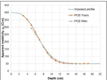
Figure 6. Simulated apparent resistivity profiles for the Transmission and Wenner configurations, 236
compared to the imposed resistivity profile. 237
In order to compare the sensor’s ability to match the resistivity profile imposed in the model 238
(equation 3), we plotted the resistivity profile in Figure 6 as a function of depth for both the 239
Transmission and the Wenner configurations. It is obvious from this figure that the relative difference 240
between the actual resistivity distribution (imposed profile) and the simulated apparent resistivities is 241
very small. The normalized mean root squared error (NRMSE) was calculated between the imposed 242
profile and the calculated profiles of the PCB sensor. We found an NRMSE of 0.36% for the 243
Transmission configuration, and 3.98% for the Wenner configuration. The greater difference 244
observed for the Wenner configuration may be explained by the difference in the volume investigated 245
in the Wenner and the Transmission configurations. Therefore, with the Wenner configuration, a 246
numerical inversion procedure may be required to obtain the true resistivity profile [31]. However, 247
this promising result proves the ability of the designed sensor to determine the electrical resistivity 248
profile with good resolution for both configurations. 249
4.2 Experimental validation in brine solutions
250
The objective here was to assess the repeatability of the measurements, through laboratory 251
measurements acquired in homogeneous solutions (i.e. with negligible resistivity variation) in a range 252
of known conductivities. A measurement sequence for the Wenner and Transmission configurations 253
was programmed on a commercial resistivity meter (Syscal Pro, Iris Instruments) and all the 254
measurements were made automatically. 255
4.2.1 Experimental set up
256
The PCB sensor was placed at the center of a water-filled cubic tank of dimensions 30x30x30 cm3
257
(Figure 7) between two stainless steel grids, each at a distance of 5 mm from the side surface. New 258
geometric factors were then calculated by a numerical simulation taking the new geometry of the 259
medium into account. The sensor was validated by testing various brine solutions of known resistivity 260
(the inverse of conductivity). To obtain the five solutions presented in Table 1, we gradually added 261
NaCl salt to demineralized water. The corresponding expected resistivity for each solution was 262
determined using Abacus software [49]. The values were then compared to those obtained by a 263
commercial conductivity probe (WTW Multi 348i), calibrated just before the measurements were 264
carried out. In addition, reproducibility tests performed with an internal quality control solution as 265
specified in standard XPT 90-220, based on inter-laboratory tests in which the French institute 266
IFSTTAR participated, evaluated the measurement uncertainty of the conductivity probe at 3%. The 267
experimental study was performed at a constant temperature of 20 ± 1 °C. 268
Table 1. Characteristics of the five electrolytes used. 269
Solution 1 Solution 2 Solution 3 Solution 4 Solution 5
Concentration NaCl (mg/l) 10 50 90 200 1000 ρ expected (Ω·m) (no value on the abacus) 100 63 25 5.5 270
Figure 7. The PCB sensor and stainless steel grids tested in a brine solution. 271
4.2.2 Results and discussion
272
The repeatability was assessed by taking three measurements per quadrupole. Table 2 presents the 273
average and standard deviation of the resistivity measured with the PCB sensor in the Transmission 274
and Wenner configurations for all solutions. Solution 1, with low NaCl concentration, was excluded 275
since it had higher repeatability variation (1.7% for the Wenner configuration). The coefficient of 276
variation, CV, for the repeatability with solutions 2 to 5 varied from 0.2% to 0.6% and the CV for the 277
variability along the sensor line varied from 0.7% to 1.2%. All the results are detailed in Table 2. 278
Figure 8 presents the variation of the resistivity profiles over depth for the PCB sensor (Transmission 279
and Wenner configurations) and conductivity probe for solutions 2, 3, 4 and 5. 280
An average relative difference of 2.6% can be observed between the expected resistivity and that 281
measured with the conductivity probe. What is more, no significant degradation of the results over 282
time was observed that might have been associated with the change in the composition of the solution 283
by carbonation of the exchange surface. 284
(a)
(c)
(b)
(d)
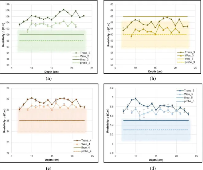
Figure 8. Variation of the resistivity profiles over depth for the PCB sensor (Transmission and Wenner 286
configurations) and the conductivity probe (uncertainty of the probe is highlighted): (a) solution 2; (b) solution 287
3; (c) solution 4; (d) solution 5. 288
Table 2. Electrical resistivity measured with the conductivity probe and the PCB sensor in the 289
Transmission and Wenner configurations for the five solutions. 290
Solution 1 Solution 2 Solution 3 Solution 4 Solution 5
Conductivity probe ρ (Ω·m) 450 ± 13 98 ± 3 60 ± 2 25 ± 1 5.3 ± 0.2 PCB Trans ρ (Ω·m) CV repeatability (%) CV variability (%) 484.6 ± 1.4 0.3 2.9 105.9 ± 0.2 0.2 1.2 61.8 ± 0.2 0.3 1.0 26.7 ± 0.1 0.4 1.2 5.8 ± 0.03 0.5 1.5 PCB Wen ρ (Ω·m) CV repeatability (%) CV variability (%) 448.3 ± 7.4 1.7 1.0 103.4 ± 0.4 0.4 0.8 60.6 ± 0.2 0.3 0.8 26.3 ± 0.1 0.4 0.7 5.7 ± 0.03 0.6 0.8 The results in Table 2 and Figure 8 show that values for the resistivity measured with the PCB sensor 291
are in good agreement with the conductivity probe measurements; on average for all solutions, a 292
relative difference of 6.8% is calculated for the Transmission configuration and 4.8% for the Wenner 293
configuration. Good correlation was found between measurements of the PCB sensor and the 294
conductivity probe, as can be seen in Figure 9. These performances are equivalent to the state of the 295
art [6] with surface measurements. 296
297
Figure 9. Correlation between the resistivity measured with the PCB sensor for the Wenner and 298
Transmission configurations and the resistivity measured with the commercial probe. 299
4.3 Experimental validation in concrete specimen
300
This part of the study deals with the experimental validation of the sensor in a concrete specimen, the 301
target material. We first demonstrate the ability to measure the concrete resistivity, then check the 302
variability and repeatability of the measurements. In addition, the response of the sensor to concrete 303
drying is studied. At the end of the experiments, a splitting tensile strength test was carried out on a 304
specimen to visually check the contact between the electrodes and the concrete. 305
4.3.1 Experimental set up
306
The concrete used in this study was based on cement type 1 (CEM I) with a water-cement ratio of 0.59 307
and a porosity of 15.0% ± 0.9%. Five cylindrical specimens of diameter 11 cm and length 22 cm were 308
used to quantify the variability of the measurement with the same sensor in all specimens. The PCB 309
sensor was placed at the center of the cylinder and the grids (Figure 2) were placed on the external 310
surfaces of the mold, embedded in the concrete at a depth of 5 mm as in the numerical model (section 311
4.1). Tests were conducted after 28 days of curing, two concrete specimens were then dried at 20 °C 312
for 28 days, followed by drying at 45 °C to accelerate the establishment of a resistivity profile. The 313
cylinders were sealed with aluminum foil on the lateral and the underside faces; only the upper face 314
was kept in contact with the air to ensure a unidirectional drying. Conditions were thus close to the 315
drying conditions of a full-scale structure. 316
4.3.2 Characterization of the sensor in concrete
317
The repeatability assessment for the resistance measured over time showed a stable resistance value 318
for three measurements made 5 minutes apart in saturated conditions. The coefficient of variation 319
ranged between 0.07% and 1.86% for the Transmission configuration, and between 0.06% and 0.75% 320
for the Wenner configuration. In addition, the coefficient of variation CV for the variability along the 321
sensor line varied from 4.3% to 6.7% for the Transmission configuration, and from 2.5% to 5.7% for 322
the Wenner configuration. 323
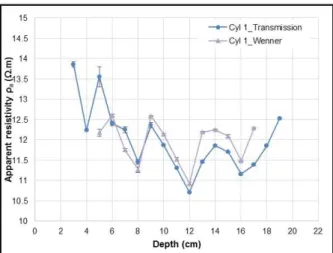
To compare the Transmission and Wenner configurations, the apparent resistivity profiles for 324
cylinder 1 in saturated conditions are plotted in Figure 10. It can be observed that both configurations 325
have the same profile and follow similar trends (minima, maxima, changes of slope), which shows 326
that they are sensitive to the same parameters at each depth (state and variability of the concrete, state 327
of the contacts, etc.) although different apparent resistivity values ρa were measured. An NRMSE of
328
4.76% was calculated between the two configurations. This calls into question the initial idea of 329
estimating the depth of the resistance measurement at the middle of the electrodes, where the potential 330
is measured, especially for the Wenner configuration (see the numerical modeling in section 4.1). 331
332
Figure 10. Apparent resistivity profile according to depth using the Transmission and Wenner 333
configurations in saturated conditions for cylinder 1. 334
The reproducibility was assessed by testing the sensor’s response variability in all cylindrical 335
specimens subjected to the same laboratory conditions. The reproducibility here is associated with 336
variation due to the sensor and concrete material variability. Figure 11 shows the variation of the 337
apparent resistivity profile with depth for all specimens, using the Transmission configuration in 338
saturated conditions. The apparent relative variation of resistivity is 4.6% on average between 339
cylinders 1, 3, 4 and 5, and 11.1% for all cylinders including cylinder 2, which has higher resistivity 340
values. These ranges of CV for the reproducibility measurements in concrete are similar to those 341
reported by Morris [50] (4% to 11%) with a surface Wenner probe in saturated conditions. According 342
to Andrade et al. [32], a CV of 10% is good and 20% is acceptable for controlled conditions, while up 343
to 30% is normal for on-site conditions. 344
Therefore, for this case study, it can be concluded that the PCB sensor developed yields results within 345
an acceptable range of variability. 346
(a) (b)
Figure 11. Apparent resistivity profile over depth using the Transmission configuration in saturated 347
conditions: (a) all cylinders; (b) average profile with the minimum and maximum profiles. 348
In order to test the sensitivity of the sensor to drying, the variation of the apparent resistivity profile 349
with time is illustrated in Figure 12 for the Transmission configuration, where t0 marks the beginning 350
of concrete drying at 20 °C and t’0 marks the beginning of concrete drying at 45 °C. In Figure 12, the 351
relative apparent resistivity variation ∆ρ for each depth was calculated relative to a reference time 352
using equation 5: 353
∆ρ =ρ$− ρ %&'
ρ %&' (5)
where ρ$ is the apparent resisitivity value at a time t and ρ %&' is the apparent resisitivity value 354
measured at the beginning of each drying process (t0 in Figure 12.a and t’0 in Figure 12.b 355
respectively). 356
The measured apparent resistivity shows a general increase over time, which implies a decrease of the 357
water content due to the drying process. The water content profile created between the two faces of 358
the cylinder is caused by the evaporation of the water from the face that is in contact with the air. We 359
observe in Figure 12 that the relative apparent resistivity variation near the surface is higher than that 360
at the heart. This is due to the unidirectional drying of the concrete. Similar tendencies have been 361
observed in previous studies concerning the determination of water content gradients, such as 362
[7,13,14]. In addition, when the drying was accelerated at 45 °C (Figure 12.b), the relative apparent 363
resistivity variation increased more rapidly near the surface. This demonstrates the ability of the 364
designed sensor to monitor the resistivity profile due to concrete drying with a spatial resolution of 365
about 1cm. 366
For very low degrees of saturation (less than 30–40% according to Lataste et al. in [12], even 20-30% 367
for certain concrete mixes), the hydric continuity is not sufficient in the porosity and the resistivity 368
becomes too high (between 2000 and 4000 Ω·m) to be measured by available commercial resistivity 369
meters. However, in the study presented herein, such very low degrees of saturation have not yet been 370
reached after 2 years of drying in conditions corresponding to thick concrete structures. 371
(a) (b)
Figure 12. Relative apparent resistivity variation profile over depth using the Transmission configuration 372
during the drying of the concrete specimen: (a) at 20 °C; (b) at 45 °C. 373
4.3.3 Visual check of the contact between electrodes and concrete
374
A splitting tensile strength test was carried out on one concrete specimen to visually verify the contact 375
between the PCB sensor electrodes and the concrete. Figure 13 shows a photograph of the splitting of 376
the concrete specimen with a close-up on the electrodes and their footprints left in the concrete. 377
Good contact is observed between all electrodes (PCB electrodes and grids) and the concrete, 378
verifying the adhesion between the concrete and the PCB sensor, which does not present any sign of 379
alteration. The aggregates were able to penetrate between two consecutive electrodes and to pass 380
through the grids well (previous assumption). The contact resistances measured between pairs of 381
electrodes varied from 7 kΩ (beginning of drying) to 35 kΩ (end of drying), and from 2 kΩ 382
(beginning of drying) to 10 kΩ (end of drying) on the grids. The influence of the PCB sensor on the 383
concrete strength can be considered as minimal in the application of the thick concrete repository 384
structures used for radioactive wastes since the volume of the sensor is small compared to the global 385
volume of the structure. 386
(a) (b)
Figure 13. Photos of the split concrete specimen: (a) general view of the PCB sensor and the grids; (b) 387
close-up on the electrodes (top) and their footprints in the concrete (bottom). 388
5 VALIDATION WITH GAMMADENSIMETRY DATA AND DISCUSSION 389
Gammadensimetry is a method commonly used to check concrete density [16,17]. It is also used to 390
determine water content profiles. By taking the water loss into account in the calculation of the mass 391
absorption coefficient, the accuracy of the parameter characterizing the concrete internal water 392
content is improved [16]. It is based on the material’s absorption of gamma rays emitted by a Cesium 393
137 radioactive source. The diameter of the test specimen used here was 11cm and its height was 30 394
cm. It was sealed with aluminium foil and exposed to drying conditions similar to those of the 395
cylindrical specimens where the PCB resistivity sensor was embedded. It was placed with a rotational 396
movement about its axis: the measurement corresponded to the average over a slice of concrete 397
having an estimated thickness of 10 mm. One measurement was made every 6 mm. The uncertainty of 398
gammadensimetry values is estimated at 0.5%. We calculated the relative density variationsfor each 399
depth and each time in both drying processes (at 20 °C and 45 °C) relative to an initial state (reference 400
time) using a simple expression (similar to Eq. (5)). The results are plotted in Figure 14, where T0 401
marks the initial saturated state and the beginning of concrete drying at 20 °C and T’0=T0+146 days 402
marks the beginning of concrete drying at 45 °C. 403
(a) (b)
Figure 14. Relative density variation over depth during the drying of the concrete specimens: (a) at 404
20 °C; (b) at 45 °C. 405
An increase in the relative density variation is observed over time, revealing the drying of the 406
concrete. The relative density variation on the surface at 20 °C is equal to 0.6% for t0+2 days and 407
2.3% for t0+146 days. At 45 °C, the relative density on the surface varies between 2.3% and 3.8% 408
over 42 days. The concrete took a very long time to dry even after the temperature increase. To make 409
a comparison between the relative density and apparent resistivity variations (using the Transmission 410
configuration) with depth, Figure 15 shows both variations plotted on the same graph for certain 411
common times within the drying process. 412
413
414
Figure 15. Relative density (left axis) and apparent resistivity (right axis) variations over the concrete 415
specimen depth. 416
Gammadensimetry makes it possible to monitor the drying of the concrete [16] and correlates well 417
with the relative apparent resistivity variation profiles over time. Similar variations can also be 418
observed in Figure 15 for the density and apparent resistivity measured in the concrete. According to 419
our results, the PCB sensor sensitivity varies from 10 to 40 ± 10 Ω·m for a saturation degree variation 420
from 100 to 73 ± 5% (calculated by gammadensimetry). Considering results given in the literature 421
[6,7] and Archie’s law [51], the sensitivity range should be higher for lower saturation degrees, when 422
the drying is at an advanced stage. Therefore, further research should include long-term drying to 423
achieve lower saturation degrees and extend our results. 424
6 CONCLUSIONS 425
In this paper, a PCB sensor based on an electrical resistivity technique has been developed to evaluate 426
the resistivity profile in concrete in order to monitor moisture gradients in real structures. The 427
embedded sensor presents various advantages, such as measuring profiles at the centimeter scale over 428
the thickness of a concrete structure; ensuring good electrical contacts between the electrodes and the 429
concrete, which is optimal for monitoring purposes; having good precision and low fabrication cost 430
and reducing the handling of wiring. A numerical study was conducted to validate the sensor’s 431
response. Results show that apparent resistivity profiles simulated for the Transmission and Wenner 432
configurations are quite close to the actual resistivity profile. Experimental measurements were 433
carried out on electrolytes of known conductivities and the sensor proved its ability to determine 434
resistivity values accurately. Moreover, a validation of the PCB sensor was carried out on concrete 435
cylindrical specimens and the apparent resistivity profile was monitored at different times of drying. 436
The apparent resistivity data were shown to be sensitive to the evolution of concrete while it was 437
drying over time. The results are validated by comparison with independently measured 438
gammadensimetry data. In the future, we plan to optimize the measurement configurations using the 439
sensitivity study. The PCB sensor may be used in many structures to monitor resistivity profiles and, 440
more importantly, moisture content profiles by means of material-dependent calibration. 441
Acknowledgments: The authors are grateful to Jean-Luc Geffard from the Materials and Structures 442
department in IFSTTAR and Carole Soula from the Laboratory of Materials and Durability of 443
Constructions (LMDC) for the technical support they provided. Our thanks are extended to Susan 444
Becker, a native English speaker, commissioned to proofread the final English version of this paper. 445
References
446
[1] T. Bore, N. Wagner, S. Delepine Lesoille, F. Taillade, G. Six, F. Daout, D. Placko, Error 447
Analysis of Clay-Rock Water Content Estimation with Broadband High-Frequency 448
Electromagnetic Sensors—Air Gap Effect, Sensors. 16 (2016) 554. doi:10.3390/s16040554. 449
[2] R. Farhoud, J. Bertrand, S. Buschaert, S. Delepine-Lesoille, G. Hermand, Full scale in situ 450
monitoring section test in the Andra’s Underground Research Laboratory, in: Proceedings of 451
the 1st Conference on Technological Innovations in Nuclear Civil Engineering (TINCE), Paris, 452
France, 2013: pp. 29–31. 453
[3] A. Courtois, T. Clauzon, F. Taillade, G. Martin, Water Content Monitoring for Flamanville 3 454
EPR TM Prestressed Concrete Containment: an Application for TDR Techniques, (2015). 455
[4] S. Arsoy, M. Ozgur, E. Keskin, C. Yilmaz, Enhancing TDR based water content measurements 456
by ANN in sandy soils, Geoderma. 195 (2013) 133–144. 457
[5] X. Dérobert, J. Iaquinta, G. Klysz, J.-P. Balayssac, Use of capacitive and GPR techniques for 458
the non-destructive evaluation of cover concrete, NDT & E International. 41 (2008) 44–52. 459
[6] R. Du Plooy, S.P. Lopes, G. Villain, X. Derobert, Development of a multi-ring resistivity cell 460
and multi-electrode resistivity probe for investigation of cover concrete condition, NDT & E 461
International. 54 (2013) 27–36. 462
[7] M. Fares, G. Villain, Y. Fargier, M. Thiery, X. Derobert, S. Palma-Lopes, Estimation of water 463
gradient and concrete durability indicators using capacitive and electrical probes, in: NDT-CE 464
2015, International Symposium Non-Destructive Testing in Civil Engineering, 2015: p. 9p. 465
[8] Z.M. Sbartaï, S. Laurens, J. Rhazi, J.P. Balayssac, G. Arliguie, Using radar direct wave for 466
concrete condition assessment: Correlation with electrical resistivity, Journal of Applied 467
Geophysics. 62 (2007) 361–374. 468
[9] A. Ihamouten, G. Villain, X. Derobert, Complex permittivity frequency variations from 469
multioffset GPR data: Hydraulic concrete characterization, IEEE Transactions on 470
Instrumentation and Measurement. 61 (2012) 1636–1648. 471
[10] İ. Kaplanvural, E. Pekşen, K. Özkap, Volumetric water content estimation of C-30 concrete 472
using GPR, Construction and Building Materials. 166 (2018) 141–146. 473
[11] S.G. Millard, Reinforced concrete resistivity measurement techniques, in: Institution of Civil 474
Engineers, Proceedings, 1991. 475
[12] J.-P. Balayssac, V. Garnier, Non-destructive testing and evaluation of civil engineering 476
structures, Elsevier, 2017. 477
[13] G. Villain, Z.M. Sbartaï, J.-F. Lataste, V. Garnier, X. Dérobert, O. Abraham, S. Bonnet, J.-P. 478
Balayssac, N.T. Nguyen, M. Fares, Characterization of water gradients in concrete by 479
complementary NDT methods, in: International Symposium Non-Destructive Testing in Civil 480
Engineering (NDT-CE 2015), 2015: p. 12p. 481
[14] J.-P. Balayssac, V. Garnier, G. Villain, Z.-M. Sbartaï, X. Dérobert, B. Piwakowski, D. Breysse, 482
J. Salin, An overview of 15 years of French collaborative projects for the characterization of 483
concrete properties by combining NDT methods, in: Proceedings of Int. Symp. on NDT-CE, 484
2015: pp. 15–17. 485
[15] H. Minagawa, S. Miyamoto, M. Hisada, Relationship of Apparent Electrical Resistivity 486
Measured by Four-Probe Method with Water Content Distribution in Concrete, Journal of 487
Advanced Concrete Technology. 15 (2017) 278–289. 488
[16] G. Villain, M. Thiery, Gammadensimetry: A method to determine drying and carbonation 489
profiles in concrete, Ndt & E International. 39 (2006) 328–337. 490
[17] G. Villain, M. Thiery, G. Platret, Measurement methods of carbonation profiles in concrete: 491
Thermogravimetry, chemical analysis and gammadensimetry, Cement and Concrete Research. 492
37 (2007) 1182–1192. doi:10.1016/j.cemconres.2007.04.015. 493
[18] M. Albrand, G. Klysz, X. Ferrieres, P. Millot, Evaluation of the electromagnetic properties of 494
non-homogeneous concrete by inversion of GPR measurements, in: 2016 16th International 495
Conference on Ground Penetrating Radar (GPR), Ieee, Hong-Kong, 2016: pp. 1–4. 496
[19] X. Xiao, A. Ihamouten, G. Villain, X. Dérobert, Use of electromagnetic two-layer wave-guided 497
propagation in the GPR frequency range to characterize water transfer in concrete, NDT & E 498
International. 86 (2017) 164–174. doi:10.1016/j.ndteint.2016.08.001. 499
[20] B. Guan, A. Ihamouten, X. Dérobert, D. Guilbert, S. Lambot, G. Villain, Near-Field 500
Full-Waveform Inversion of Ground-Penetrating Radar Data to Monitor the Water Front in 501
Limestone, IEEE Journal of Selected Topics in Applied Earth Observations and Remote 502
Sensing. 10 (2017) 4328–4336. doi:10.1109/JSTARS.2017.2743215. 503
[21] M. Chouteau, S. Vallières, E. Toe, A multi-dipole mobile array for the non-destructive 504
evaluation of pavement and concrete infrastructures: a feasability study, in: Proceedings of the 505
BAM International Symposium NDT-CE, Berlin, Germany, 2003: pp. 16–19. 506
[22] R.B. Polder, Critical chloride content for reinforced concrete and its relationship to concrete 507
resistivity, Materials and Corrosion. 60 (2009) 623–630. doi:10.1002/maco.200905302. 508
[23] M. Fares, G. Villain, S. Bonnet, S. Palma Lopes, B. Thauvin, M. Thiery, Determining chloride 509
content profiles in concrete using an electrical resistivity tomography device, Cement and 510
Concrete Composites. 94 (2018) 315–326. doi:10.1016/j.cemconcomp.2018.08.001. 511
[24] K. Hornbostel, C.K. Larsen, M.R. Geiker, Relationship between concrete resistivity and 512
corrosion rate – A literature review, Cement and Concrete Composites. 39 (2013) 60–72. 513
doi:10.1016/j.cemconcomp.2013.03.019. 514
[25] A.Q. Nguyen, G. Klysz, F. Deby, J.-P. Balayssac, Evaluation of water content gradient using a 515
new configuration of linear array four-point probe for electrical resistivity measurement, 516
Cement and Concrete Composites. 83 (2017) 308–322.
517
doi:10.1016/j.cemconcomp.2017.07.020. 518
[26] G. Villain, V. Garnier, Z.M. Sbartaï, X. Derobert, J.-P. Balayssac, Development of a calibration 519
methodology to improve the on-site non-destructive evaluation of concrete durability 520
indicators, Materials and Structures. 51 (2018) 40. 521
[27] S.E.S. Mendes, R.L.N. Oliveira, C. Cremonez, E. Pereira, E. Pereira, R.A. Medeiros-Junior, 522
Electrical resistivity as a durability parameter for concrete design: Experimental data versus 523
estimation by mathematical model, Construction and Building Materials. 192 (2018) 610–620. 524
doi:10.1016/j.conbuildmat.2018.10.145. 525
[28] C. Rücker, T. Günther, The simulation of finite ERT electrodes using the complete electrode 526
model, Geophysics. 76 (2011) F227–F238. 527
[29] K. Gowers, S. Millard, Measurement of concrete resistivity for assessment of corrosion, ACI 528
Materials Journal. 96 (1999). 529
[30] F. Wenner, A method for measuring earth resistivity, Journal of the Washington Academy of 530
Sciences. 5 (1915) 561–563. 531
[31] R.B. Polder, Test methods for on site measurement of resistivity of concrete — a RILEM 532
TC-154 technical recommendation, Construction and Building Materials. 15 (2001) 125–131. 533
doi:10.1016/S0950-0618(00)00061-1. 534
[32] C. Andrade, R. Polder, M. Basheer, Non-destructive methods to measure ion migration, RILEM 535
TC. (2007) 91–112. 536
[33] L. Bourreau, V. Bouteiller, F. Schoefs, L. Gaillet, B. Thauvin, J. Schneider, S. Naar, 537
Uncertainty assessment of concrete electrical resistivity measurements on a coastal bridge, 538
Structure and Infrastructure Engineering. 15 (2019) 443–453. 539
doi:10.1080/15732479.2018.1557703. 540
[34] J. Priou, Y. Lecieux, M. Chevreuil, V. Gaillard, C. Lupi, D. Leduc, E. Rozière, R. Guyard, F. 541
Schoefs, In situ DC electrical resistivity mapping performed in a reinforced concrete wharf 542
using embedded sensors, Construction and Building Materials. 211 (2019) 244–260. 543
doi:10.1016/j.conbuildmat.2019.03.152. 544
[35] L. Marescot, S. Rigobert, S.P. Lopes, R. Lagabrielle, D. Chapellier, A general approach for DC 545
apparent resistivity evaluation on arbitrarily shaped 3D structures, Journal of Applied 546
Geophysics. 60 (2006) 55–67. 547
[36] G. Kunetz, Principles of direct current-Resistivity prospecting, (1966). 548
[37] G.A. Oldenborger, P.S. Routh, M.D. Knoll, Sensitivity of electrical resistivity tomography data 549
to electrode position errors, Geophysical Journal International. 163 (2005) 1–9. 550
[38] C.-Y. Chang, S.-S. Hung, Implementing RFIC and sensor technology to measure temperature 551
and humidity inside concrete structures, Construction and Building Materials. 26 (2012) 628– 552
637. 553
[39] D. LaBrecque, W. Daily, Assessment of measurement errors for galvanic-resistivity electrodes 554
of different composition, Geophysics. 73 (2008) F55–F64. 555
[40] K. Liang, X. Zeng, X. Zhou, C. Ling, P. Wang, K. Li, S. Ya, Investigation of the capillary rise in 556
cement-based materials by using electrical resistivity measurement, Construction and Building 557
Materials. 173 (2018) 811–819. 558
[41] Y. Abbas, F. Pargar, W. Olthuis, A. van den Berg, Activated carbon as a pseudo-reference 559
electrode for potentiometric sensing inside concrete, Procedia Engineering. 87 (2014) 1437– 560
1440. 561
[42] M. Petrič, S. Kastelica, P. Mrvar, Selection of electrodes for the’in situ’electrical resistivity 562
measurements of molten aluminium, Journal of Mining and Metallurgy B: Metallurgy. 49 563
(2013) 279–283. 564
[43] O. Kuras, P.B. Wilkinson, P.I. Meldrum, R.T. Swift, S.S. Uhlemann, J.E. Chambers, F.C. 565
Walsh, J.A. Wharton, N. Atherton, Performance Assessment of Novel Electrode Materials for 566
Long-term ERT Monitoring, in: Near Surface Geoscience 2015-21st European Meeting of 567
Environmental and Engineering Geophysics, 2015. 568
[44] J. Song, L. Wang, A. Zibart, C. Koch, Corrosion protection of electrically conductive surfaces, 569
Metals. 2 (2012) 450–477. 570
[45] L.S. Edward, A modified pseudo section for resistivity and induced-polarization, Geophysics. 571
42 (1977) 1020–1036. 572
[46] M. Loke, Electrical Imaging Surveys for Environmental and Engineering Studies, 2000. 573
[47] S.K. Park, G.P. Van, Inversion of pole‐pole data for 3-D resistivity structure beneath arrays of 574
electrodes, GEOPHYSICS. 56 (1991) 951–960. doi:10.1190/1.1443128. 575
[48] W.J. McCarter, H.M. Taha, B. Suryanto, G. Starrs, Two-point concrete resistivity 576
measurements: interfacial phenomena at the electrode–concrete contact zone, Measurement 577
Science and Technology. 26 (2015) 085007. 578
[49] D. Chapellier, Diagraphies appliquées à l’hydrologie, technique et documentation (Lavoisier), 579
Diagraphies, 1987. 580
[50] W. Morris, E.I. Moreno, A.A. Sagüés, Practical evaluation of resistivity of concrete in test 581
cylinders using a Wenner array probe, Cement and Concrete Research. 26 (1996) 1779–1787. 582
[51] G.E. Archie, The electrical resistivity log as an aid in determining some reservoir 583
characteristics, Transactions of the American Institute of Mining and Metallurgical Engineers. 584
(1942) 54–62. 585