Observations of iodine monoxide (IO) columns from satellite

(1)

HAL Id: hal-00303084

https://hal.archives-ouvertes.fr/hal-00303084

Submitted on 5 Sep 2007

HAL is a multi-disciplinary open access

archive for the deposit and dissemination of sci-entific research documents, whether they are pub-lished or not. The documents may come from teaching and research institutions in France or abroad, or from public or private research centers.

L’archive ouverte pluridisciplinaire HAL, est destinée au dépôt et à la diffusion de documents scientifiques de niveau recherche, publiés ou non, émanant des établissements d’enseignement et de recherche français ou étrangers, des laboratoires publics ou privés.

Observations of iodine monoxide (IO) columns from

satellite

A. Schönhardt, A. Richter, F. Wittrock, H. Kirk, H. Oetjen, H. K. Roscoe, J.

P. Burrows

To cite this version:

A. Schönhardt, A. Richter, F. Wittrock, H. Kirk, H. Oetjen, et al.. Observations of iodine monoxide (IO) columns from satellite. Atmospheric Chemistry and Physics Discussions, European Geosciences Union, 2007, 7 (5), pp.12959-12999. �hal-00303084�

(2)

ACPD

7, 12959–12999, 2007

Observations of iodine monoxide (IO)

columns from satellite A. Sch ¨onhardt et al. Title Page Abstract Introduction Conclusions References Tables Figures ◭ ◮ ◭ ◮ Back Close

Full Screen / Esc

Printer-friendly Version

Interactive Discussion Atmos. Chem. Phys. Discuss., 7, 12959–12999, 2007

www.atmos-chem-phys-discuss.net/7/12959/2007/ © Author(s) 2007. This work is licensed

under a Creative Commons License.

Atmospheric Chemistry and Physics Discussions

Observations of iodine monoxide (IO)

columns from satellite

A. Sch ¨onhardt1, A. Richter1, F. Wittrock1, H. Kirk1, H. Oetjen1,*, H. K. Roscoe2, and J. P. Burrows1

1

Institute of Environmental Physics, University of Bremen, Otto-Hahn-Allee 1, 28359 Bremen, Germany

2

British Antarctic Survey, Natural Environment Research Council, High Cross, Madingley Road, Cambridge CB3 0ET, UK

*

now at: School of Chemistry, University of Leeds, Leeds, LS2 9JT, UK

Received: 23 July 2007 – Accepted: 31 August 2007 – Published: 5 September 2007 Correspondence to: A. Sch ¨onhardt ([email protected])

(3)

ACPD

7, 12959–12999, 2007

Full Screen / Esc

Interactive Discussion

Abstract

Iodine species in the troposphere are linked to ozone depletion and new particle forma-tion. In this study, a full year of iodine monoxide (IO) columns retrieved from measure-ments of the SCIAMACHY satellite instrument is presented, alongside a discussion of their uncertainties and the detection limit. The largest amounts of IO are found near

5

springtime Antarctica, where ground-based measurements have positively detected iodine compounds before. A seasonal variation of iodine monoxide in Antarctica is re-vealed with high values in springtime, slightly less IO in the summer period and again larger amounts in autumn. In winter, no elevated IO levels are found in the areas acces-sible to satellite measurements. This seasonal cycle is in good agreement with recent

10

ground-based measurements in Antarctica. In the Arctic region, no elevated IO levels were found in the whole time period analysed, arguing for different conditions existing in the two Polar Regions. To investigate possible release mechanisms such as inorganic release or biogenic precursors, comparisons of IO results with tropospheric BrO maps, measurements of chlorophyll concentration, and ice coverage are discussed. Some

15

parallels and interesting differences between IO and BrO temporal and spatial distribu-tions are pointed out. Although no full interpretation can be given at this point, the large spatial coverage of satellite measurements and the availability of a long-term dataset give some new indications and understandings of the abundances and distributions of iodine compounds in the troposphere.

20

1 Introduction

In recent times, measurements in the atmosphere and related model studies have re-vealed the relevance of iodine species in the chemistry of the troposphere and the planetary boundary layer (Alicke et al.,1999;Vogt et al.,1999;Carpenter et al.,2003). Atmospheric models and measurement methods to determine iodine compounds in the

25

atmosphere were initially developed on account of radioactive iodine isotopes released 12960

(4)

ACPD

7, 12959–12999, 2007

Full Screen / Esc

Interactive Discussion from nuclear power installations and the need to understand their distribution and

de-position (Chamberlain and Chadwick, 1953; Chamberlain,1960;Chamberlain et al., 1960). Models for the investigation of tropospheric iodine chemistry further evolved af-ter the recognition of significant release of methyl iodide into the troposphere ( Chamei-des and Davis, 1980;Chatfield and Crutzen,1990). The importance of iodine in the

5

atmosphere includes its role in tropospheric ozone depletion and its influence on new particle formation (O’Dowd et al.,1999,2002a,b;McFiggans et al.,2004). The poten-tial significance of iodine for stratospheric chemistry has also been studied (Solomon et al.,1994). Information about the spatial and temporal distribution of iodine compounds is required to assess accurately their role in atmospheric chemistry, but is currently

10

limited by the sparseness of available measurements. In this context, the detection of iodine monoxide (IO) from instrumentation aboard orbiting satellites has the potential to fill in part this gap and thereby test and improve our understanding of iodine chemistry. During the last decade, IO has been observed in a variety of atmospheric studies, primarily in the marine boundary layer (Alicke et al.,1999;Carpenter et al.,1999;Peters

15

et al.,2005) in polar regions (Wittrock et al.,2000;Friess et al., 2001;Saiz-Lopez et al.,2007a), and also above the open ocean (Allan et al.,2000). In addition to IO, other relevant iodine compounds such as the iodine dioxide molecule OIO, molecular iodine I₂, and organic iodocarbons have also been observed in the troposphere (Carpenter et al.,1999;Saiz-Lopez et al.,2006). In coastal areas, I₂and volatile organic iodocarbons

20

including CH₃I, CH₂I₂and CH₂ICl emitted directly or indirectly from algae, are thought to be the typical precursors of atomic iodine. At mid-latitudes, such as Mace Head in Ireland, a correlation of IO with solar irradiation and low tidal height exposing the emitting algae to air was identified (Alicke et al.,1999;Carpenter et al.,1999;Peters et al.,2005).

25

Also in Polar Regions, the source of iodine is partly attributed to release of iodine containing organic compounds from ice algae (Reifenh ¨auser and Heuman,1992; Car-penter et al.,2007). However, inorganic mechanisms releasing iodine from sea salt or brine cannot be ruled out (Carpenter et al., 2005). In any case, effective and iodine

(5)

ACPD

7, 12959–12999, 2007

Full Screen / Esc

Interactive Discussion selective release from ocean water into the atmosphere via biogenic or non-biogenic

pathways appears to exist at least locally. This is reflected by the enrichment of io-dine compounds in the marine boundary layer, especially in marine aerosols, when compared to for example chlorine species (Reifenh ¨auser and Heuman,1992;Vogt et al., 1999). Typical abundances of iodocarbons and subsequent iodine oxides lie in

5

the range of 0 to several pptv (Carpenter et al.,1999;Allan et al.,2000;Peters et al., 2005) and are most probably confined to the lowest layers of the atmosphere (Friess et al.,2001). In some locations the amount of IO was below the detection limit while higher values of up to 10 pptv (Peters et al.,2005;Zingler and Platt,2005) have been measured in several locations at certain times. The currently highest amounts of up

10

to 20 pptv (Saiz-Lopez et al.,2007a) and very recently 30 pptv (D. Heard, yet unpub-lished data) seem to be rather rare and transitory events, especially as the latter was observed in an in situ measurement.

In the stratosphere, iodine oxide could also contribute to ozone destruction (Solomon et al.,1994) but concentrations are expected to be low at least compared to the high

15

values observed in coastal hot spots. There has been some limited evidence for small amounts of IO in the polar spring in the northern hemispheric stratosphere, but the upper limit for stratospheric IO mixing ratios is small (Wennberg et al.,1997;Wittrock et al.,2000;B ¨osch et al.,2003). As a result, the integrated IO column amounts seen by satellite nadir observations are interpreted as tropospheric columns in this study,

20

assuming the IO to be situated in the boundary layer, in accordance with observations made so far.

When emitted into the atmosphere, many iodine compounds rapidly photolyse re-leasing atomic iodine radicals, e.g., (CH₂I₂_+hν→CH₂I+I) or (I2+hν→I+I). Following the

reaction with ozone (O₃), IO radicals then form initiating a catalytic ozone destruction cycle in areas of iodine release (Solomon et al.,1994). Atomic iodine is regenerated by different pathways, for example by the reaction with other halogen oxides (X=Br or Cl, ReactionsR2,R3), or with HO₂(Reactions R4,R5) or NO₂ (ReactionR8) and

(6)

ACPD

7, 12959–12999, 2007

Full Screen / Esc

Printer-friendly Version Interactive Discussion subsequent photolysis. I + O3→ IO + O2 (R1) XO + IO → I + X + O2 (R2) X + O3→ XO + O2 (R3) Net : 2O₃_{→ 3O}₂ I + O3→ IO + O2 IO + HO2→ HOI + O2 (R4) → OH + I + O2 (R5) HOI + hν → OH + I (R6) OH + O3→ HO2+ O2 (R7) Net : 2O₃_{→ 3O}₂ IO + NO2+ M → IONO2+ M (R8) IONO₂_{+ hν → I + NO}₃ (R9) → IO + NO2 (R10)

The photolysis of IO regenerates I atoms (and ozone) and leads to some steady state amount of IO during daytime.

IO + hν → I + O (R11)

O + O2+ M → O3+ M (R12)

If no other chemistry were considered and as a result of the rapid photolysis of iodine compounds, IO would be expected to be the dominant gas phase iodine compound in the troposphere. Similar to other halogen oxides like ClO and BrO (Molina and Rowland,1974;Stolarski and Cicerone,1974;Barrie et al.,1988), the presence of IO is linked to catalytic destruction of O₃. However, the chain length of such destruction

5

(7)

ACPD

7, 12959–12999, 2007

Full Screen / Esc

Interactive Discussion cycles depends on the termination reactions which produce higher oxides of iodine and

lead to particle formation.

In Polar Regions, springtime tropospheric ozone depletion events are frequently ob-served and have been linked to enhanced bromine amounts (Barrie et al., 1988; Olt-mans et al., 1989; Kreher et al., 1997, and references therein). The observations

5

of large clouds of BrO from satellites (Burrows et al.,1999;Wagner and Platt,1998; Richter et al.,1998) at high latitudes was followed by the suggestion that areas of po-tential frost flower coverage might be a major source region of these clouds (Kaleschke et al.,2004). The low temperatures of aerosol and possibly surface brine in such re-gions triggers the release of bromine (R. Sander et al.,2006), required to explain the

10

bromine explosion (Platt and H ¨onninger,2003). However, model studies suggest that even small amounts of iodine can play an important role in the release and recycling processes of Br atoms (Vogt et al.,1999). This further enhances the strength and im-pact of bromine explosions seen in Polar Regions, making the catalytic ozone depletion even more effective.

15

Recently, the issue of the importance of IO chemistry as a source of aerosol conden-sation nuclei has been raised. The higher oxides of IO are produced in the self-reaction of IO (Cox and Coker,1983;Cox et al.,1999;Bloss et al.,2001;G ´omez Mart´ın et al., 2007, and references therein), the two relevant reaction pathways being

IO + IO → OIO + I (R13)

IO + IO + M → I2O2+ M (R14)

Iodine oxides may be generated also by reaction pathways between IO and other halo-gen oxides (ClO or BrO) or possibly by minor channels of the reaction of IO with HO₂, e.g.:

BrO + IO → OIO + Br (R15)

HO₂_{+ IO → OIO + OH} (R16)

In any case, OIO or I₂O₂ are liberated. Subsequently, higher oxides (I_xO_y, such as 12964

(8)

ACPD

7, 12959–12999, 2007

Full Screen / Esc

Interactive Discussion I₂O₄and I₂O₅) are formed, which react further with OIO, and can then cluster and

pre-cipitate (O’Dowd et al.,2002a;McFiggans et al.,2004;O’Dowd and Hoffmann,2005). In addition, some of the higher iodine oxide clusters, being acid anhydrides, are very hygroscopic. The mechanism, by which aerosols are formed, is not yet established. However, it has been shown that the formation of higher oxides results in the

produc-5

tion of ultra-fine particles. These may then grow to small aerosols and act as cloud condensation nuclei. These processes impact on the aerosol loading and potentially the amount of clouds and therefore also on the Earth’s radiation budget and climate forcing. In addition, it is now clear that iodine plays a significant role in both the homo-geneous and heterohomo-geneous chemistry of the troposphere, at least locally.

10

The complete cycling of iodine in the atmosphere is still not well understood. Mea-surements of the global distribution of IO are needed to test our current knowledge and constrain atmospheric models describing iodine behaviour.

The present study addresses the observation of IO from space. For this purpose, the absorption of IO is retrieved from measurements of the back-scattered radiation

up-15

welling from the atmosphere taken by the SCanning Imaging Absorption SpectroMeter for Atmospheric ChartographY (SCIAMACHY), a UV-vis-NIR spectrometer onboard the ENVISAT satellite (Burrows et al.,1995;Bovensmann et al.,1999). First results from this study about the identification of IO from SCIAMACHY were presented recently (Sch ¨onhardt et al.,2007). The sensitivity and detection limit of the satellite

measure-20

ments with respect to IO in the atmospheric boundary layer are discussed, and a study of the spatial and seasonal variation of IO focussing on the southern hemispheric Polar Region is presented.

2 Instrument

The instrument SCIAMACHY is mounted on the ESA satellite ENVISAT, which was

25

launched in March 2002. The instrumental properties and mission objectives have been described in detail elsewhere (Burrows et al., 1995;Bovensmann et al.,1999).

(9)

ACPD

7, 12959–12999, 2007

Full Screen / Esc

Interactive Discussion The sun-synchronous, near-polar orbit of ENVISAT has a local equator crossing time

of 10:00 a.m. in a descending node. SCIAMACHY makes measurements of the trans-mitted, backscattered and reflected light from the Earth’s atmosphere or surface, ob-serving in nadir and limb viewing geometries, as well as in solar and lunar occultation. The light is separated into eight spectral channels measuring simultaneously, with six

5

contiguous channels between 240 and 1750 nm and two further short wave infrared channels. The alternate limb and nadir viewing coupled with a swath width of 960 km yields global coverage at the equator within six days.

In this study, the spectral absorption and scattering features in the blue part of the spectrum from the nadir measurements have been investigated. In order to optimise

10

the signal-to-noise ratio, the size of the ground scene was increased to 60 km along and 120 km across track by averaging several individual measurements. A criterion restrict-ing the solar zenith angle to less than 84◦was used to exclude observations having an intrinsic low signal-to-noise ratio and reduced sensitivity to the lower troposphere. As one special interest is to investigate the high latitude regions, cloud screening was not

15

applied. Reliable separation of clouds from ice and snow is not routinely available yet. The time period analysed covers the years 2004–2006 but focuses on 2005.

3 Iodine monoxide absorption

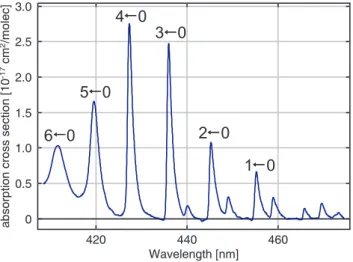
The absorption cross section of IO from its ground stateX₃2_/2 to the first electronically excited stateA2₃_/2 is shown in Fig.1. The original spectrum which was recorded with

20

a FWHM value of 0.07 nm was convoluted with the slit function of the SCIAMACHY in-strument. The IO absorption cross section reveals an extraordinarily strong differential structure in the wavelength range around 400–460 nm. For comparison, this structure is approximately two orders of magnitude larger than that for NO₂in the same spectral region which is routinely used for Differential Optical Absorption Spectroscopy (DOAS)

25

(Platt,1994) measurements of NO₂ in the troposphere and stratosphere. The maxi-12966

(10)

ACPD

7, 12959–12999, 2007

Full Screen / Esc

Interactive Discussion mum absorption cross section of IO is approximatelyσ_max(IO)=2.8×10−17_cm2_/molec

at 298 K and will be used later in the discussion of the IO detection limit of SCIAMACHY. The IO molecule is therefore an ideal trace gas for remote sensing by DOAS in spite of its lower abundance, compared to NO₂.

4 IO retrieval algorithm

5

For the retrieval of IO from SCIAMACHY data, the well-established DOAS technique has been used in this study. In this method, a polynomial acts as a high-pass filter accounting for all broadband features such as broadband absorption, scattering, and instrumental effects. All differential structures in the spectrum remain for assignment to trace gases, which exhibit highly variable absorption structures, and the Ring effect,

10

which results from the interaction of Raman scattering on air molecules with the solar Fraunhofer lines and molecular absorption features. The slant column densities are de-termined by a non-linear least squares fitting procedure for each measured spectrum. The conversion of the slant column density to a vertical column density requires the calculation of the appropriate air mass factor (AMF) determined by a radiative transfer

15

model which accounts for the light path through the trace gas layer.

The DOAS retrieval was performed in the spectral fitting window from 416 to 430 nm, which contains two absorption peaks of IO, the (ν′

=4←ν′′=0) and (ν′=5←ν′′=0) ab-sorption bands of theA2₃_/2←X₃2_/2 transition, cp. Fig. 1. A broader spectral window ex-tending to longer wavelengths including additionally the (ν′

=3←ν′′=0) band was also

20

tested. This was less successful, because of a strong Ring structure at 431 nm. As the Ring effect results in the strongest differential feature in this wavelength window for many regions on Earth, even small errors in the fitting of this effect can lead to a large and highly structured, stable residual, which can interfere with the trace gas ab-sorption for weak atmospheric abab-sorptions of IO. It was noted that this interference is

25

largest for certain geometrical conditions over bright surfaces, such as ice or clouds.

(11)

ACPD

7, 12959–12999, 2007

Full Screen / Esc

Interactive Discussion This results occasionally in large apparent IO columns but poor fitting residuals. To

avoid this problem around 431 nm, the fit was confined to the spectral bands at shorter wavelengths.

In the retrieval, a second order polynomial was applied, and absorption cross-sections from NO₂(223 K) and O₃ (223 K) (Bogumil et al.,2003), a Ring spectrum (Vountas et

5

al.,1998), as well as an undersampling correction (Chance,1998) and an additive lin-ear polynomial were included. In order to minimise the impact from the Ring effect and any residual instrument noise resulting from small differences in the viewing of the earth and the sun by the instrument, only earthshine spectra were used for fitting purposes. For the atmospheric background spectrum in the DOAS fitting procedure,

10

for each day of measurements, the earthshine spectrum from over the tropical Pacific (at 40◦S, 160◦W averaged over the available spectra within ±10◦ in both directions) was used. This is a region where the IO signal is expected to be small, which was con-firmed by fitting this earthshine signal with the solar reference spectrum. The difference in the absorption optical depth between the background spectrum and each individual

15

satellite measurement is the basis for the DOAS analysis. The resulting slant column retrieved for each single satellite pixel is the difference in slant column between the amount at a specific position and this reference position.

5 Detection limit

In order to estimate the detection limit of SCIAMACHY for IO columns, several

fac-20

tors, determined by the instrument and from assumptions in the algorithm, need to be accounted for. The minimal optical depth OD_min detectable by the instrument is determined primarily by the noise-to-signal ratio (N/S) of the measured spectrum. S is the number of electrons generated from incoming photons at the detector during a measurement, andN the value for the total noise arising in the measurement process.

25

The ratioN/S is determined by the number of photons captured in one measurement and – in the selected spectral region – to a much lesser extent by the detector noise. It

(12)

ACPD

7, 12959–12999, 2007

Full Screen / Esc

Interactive Discussion therefore depends on quantities like wavelength, surface spectral reflectance and the

solar zenith angle. For the photon signal falling on a detector pixel,N/S is given to a good approximation by the shot noise in the electron flux, i.e.,

N S = ((N 2 i + N 2 d)/S 2₎1/2

whereN_i is the number of noise electrons generated from incoming photons, andN_d is

5

the number of noise electrons determined by the dark signal for the individual detector pixel.

For the wavelength region under consideration here, the root mean square (rms) of the optical depth is on the order of 10−4 _{for 90% surface spectral reflectance (}_{No ¨el}

et al., 1998). For an ideal measurement, the slant column detection limit (SC_lim) is

10

given by the ratio of the residual rms and σ_max (the maximum differential absorption cross section value of the respective trace gas). This analysis assumes that a trace gas is detectable if the absorption optical depth SC_max_{× σ}_maxbecomes larger than the residual rms value.

For IO slant columns and a surface spectral reflectance of 90%, the detection limit

15

is given by SC_lim_=7×1012molec/cm2 for a single measurement. This limit can be fur-ther reduced by averaging, in time or space, provided the source of errors is random and systematic errors have been accounted for. For a surface spectral reflectance of 5% instead of 90%, the IO slant column detection limit for a single measurement corresponds to 2×1013molec/cm2. For 90% surface spectral reflectance and the

spa-20

tially averaged ground scene of 60×120 km2, used in this study, the limit is reduced to 3×1012molec/cm2.

To convert the slant column detection limit to a mixing ratio detection limit, assump-tions on the appropriate air mass factor, and in particular on the altitude profile of IO are necessary. For this, radiative transfer calculations using the SCIATRAN V2.0

radia-25

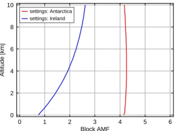
tive transfer model (Rozanov et al.,2005) have been undertaken. For the wavelength of 425 nm, the AMF varies between 1.0 (for 5% surface spectral reflectance, 55◦ solar zenith angle, as at the Irish coast) and 4.2 (for 90% surface spectral reflectance, 70◦

(13)

ACPD

7, 12959–12999, 2007

Full Screen / Esc

Interactive Discussion solar zenith angle, as in Antarctica), assuming an IO profile with constant mixing ratio

in the lowest kilometre and a linear decrease to 0 at 2 km. For the high surface spectral reflectance case, the AMF changes only by a few percent even if IO is assumed to be well mixed only in the lowest 100 m, or up to 10 km. However, for the low surface spectral reflectance case, the AMF of the two scenarios varies by a factor of 2.

5

Figure 2 shows the block AMF (the air mass factor for discrete altitude slices) for the two different settings of Antarctica and Ireland. The figure demonstrates the much larger sensitivity for the measurement of IO for typical Antarctic conditions. Up to the present no climatology of the vertical profile of IO has been determined. However, ground-based measurements have shown the tropospheric character of IO (Friess et

10

al.,2001) and indicate that IO is likely to be confined to the boundary layer. Strong evidence for confinement of Antarctic IO to the boundary layer or even the lower part of the boundary layer is also given bySaiz-Lopez et al.(2007b). As a consequence, conversion from column amount to volume mixing ratios (VMR) in the boundary layer yields detection limits of 0.7 pptv and 8 pptv, respectively, for Antarctic conditions and

15

the Irish coast for mixing up to 1 km, and, respectively, limits of 7 pptv and 80 pptv for the case that all IO is located in the lowest 100 m. All of the above values were calculated for a single measurement without any averaging. This analysis shows that the IO detection limit for a single SCIAMACHY ground scene lies close to and in some cases below the IO amounts observed by ground-based measurements. For these

20

cases, positive detection of IO from satellite can be expected if the spatial extent of the area of enhanced IO amounts is of the order of a satellite ground-pixel.

6 Results

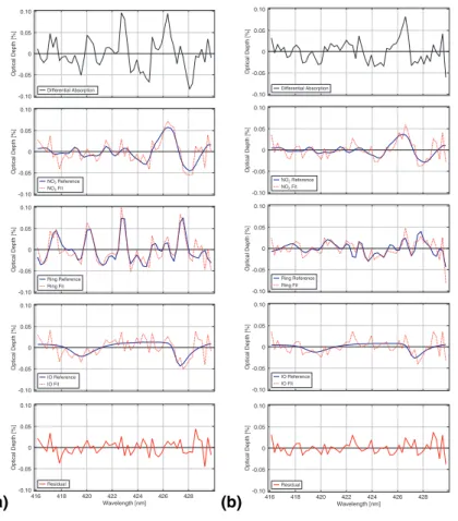
DOAS retrievals of IO were undertaken on SCIAMACHY measurements using the pro-cedure and assumptions described above. Typical fitting residuals exhibit rms values

25

of around 1–2×10−4_{in terms of optical depth for a single measurement. Two examples}

are shown in Fig. 3 for different amounts of detected IO slant columns. This figure 12970

(14)

ACPD

7, 12959–12999, 2007

Full Screen / Esc

Interactive Discussion displays the total differential absorption spectrum, the fits of NO2, the Ring effect and

IO from the measurement including in each case the residual noise in direct compar-ison with the scaled reference absorption cross section, and finally the fit residual. Assuming that a trace gas becomes detectable if its differential absorption structures are larger than the rms of the respective residual, an experimental detection limit of 5–

5

10×1012molec/cm2results for a single measurement. This limit is only slightly higher than the theoretically achievable limit discussed in the previous section. As a result of averaging the detection limit for the monthly mean drops to smaller values dependent on the square root of the number of measurements available for a specific location. This number is highly variable, ranging from no measurements at all close to the winter

10

pole to more than one measurement a day, at the summer pole. As a consequence, the detection limit in the monthly mean can improve by up to a factor of 5 or more.

Global IO slant columns averaged over the months of October and November 2005 are shown colour coded on a global map in Fig.4. The highest values in the monthly average amount to about 8×1012molec/cm2 and are detected in a widespread area

15

close to Antarctica off the coast, especially in the Weddell Sea. Other regions with enhanced values are seen e.g. over the tropical Pacific west of Central America. It is interesting to note these small amounts of IO retrieved over up welling regions and biologically active oceans. However, in these regions, the signal-to-noise ratio of the retrieval is poorer and the results for IO columns are therefore more sensitive to fit

set-20

tings. For example, a slight change in the fitting window can change these features strongly. Consequently, these values have to be treated with caution and their signif-icance will require careful validation. In contrast, the maximum close to the Antarctic continent is stable with respect to the changes in the fit settings.

Closer inspection of the figure also reveals areas with negative IO columns, mainly

25

over the “ocean deserts” where the water is clear and the penetration of solar radia-tion significant. This interference is attributed to incompletely compensated vibraradia-tional Raman scattering in water and/or weak water absorption in the water. This behaviour has been identified also in the retrievals of other trace gas products in these regions. A

(15)

ACPD

7, 12959–12999, 2007

Full Screen / Esc

Interactive Discussion more detailed modelling of the water-leaving radiance is expected to improve the fitting

results.

There is no clear indication from these results for enhanced IO columns in regions such as the Irish or Britannic coast, where ground-based measurements detected IO at high concentrations. This is probably the result of the larger detection limit at

mid-5

latitudinal coastal sites and the spatially and temporally confined nature of the sources such as the fields of algae, which emit mainly during times of low tide along the coast. For the regions outside Antarctica, an upper limit for monthly and spatially averaged IO is estimated to lie around 3×1012molec/cm2, while higher values within shorter time scales or locally might very well be present nevertheless. The results around Antarctica

10

have been further analysed and the seasonal means of the IO differential slant column are plotted in Fig.5for the Southern Hemisphere.

From this series of measurements, a seasonal variation of the Antarctic IO values is found. A regionally widespread maximum of IO values during springtime occurs throughout the Weddell Sea, in the Ross Sea and along some coastlines. In December,

15

the IO amount drops to values around and below 5×1012molec/cm2remaining close to this value for the polar summer and peaking slightly again during the autumn period around March. In this period, a higher amount of scatter is seen in the data for yet unknown reasons. In winter, there are no measurements from SCIAMACHY close to the poles due to darkness, but even at the rim of the measurement region, in areas

20

where IO exists in other times of the year, no systematically enhanced values are detected.

Very recently, a study of IO columns for four days of SCIAMACHY data has been published (Saiz-Lopez et al., 2007c). In agreement with the results presented here, high values are reported close to Antarctica in October 2005. At the same time, some

25

differences have been noticed with respect to the maximal daily IO columns, which tend to be a few times lower in the observations of the present study. Additionally, the spatial distribution differs. While enhanced values of IO spread mainly in the Weddell Sea and at the Antarctic continent here, inSaiz-Lopez et al.(2007c) the highest values

(16)

ACPD

7, 12959–12999, 2007

Full Screen / Esc

Interactive Discussion were retrieved above sea ice regions between 60◦_{and 70}◦_{Southern latitude, but in two}

cases also well outside the ice covered regions over the ocean southwest of the South American continent, possibly related to cloud fields. The reasons for these differences are yet not clear but will be investigated when a longer time series of satellite data is available from the study ofSaiz-Lopez et al.(2007c).

5

Overall, the DOAS fit yields reliable results in terms of the seasonal and spatial pat-tern, while the exact numbers of the IO slant column are subject to some remaining uncertainties. The quantitative analysis can only be further improved either by extend-ing the fittextend-ing window to include three or more IO absorption peaks, after havextend-ing solved the issues, discussed above with respect to residual features from strong Raman

struc-10

tures in that wavelength range or, by averaging of more spectra before starting the fit routine.

7 Comparison with ground-based measurements

For a validation of the retrieved IO columns from satellite, a comparison with ground-based measurements is required. In this context the seasonal variation in IO columns

15

seen from SCIAMACHY in Antarctica can be compared with some long-path DOAS (LP-DOAS) results taken at Halley Station (75.5◦_{S, 26.5}◦_{W) during the CHABLIS}

(Chem-istry of the Antarctic Boundary Layer and Interface with Snow) campaign (Saiz-Lopez et al.,2007a, and references therein), which took place from January 2004 until February 2005. Approximately at a distance of 12 km from the ocean, Halley Station is situated

20

on the Antarctic shelf ice. The LP-DOAS measurements yield the trace gas volume-mixing ratio (VMR) at 4–5 m elevation above the ice surface averaged over the optical path length of 8 km. Assuming a vertical distribution of IO, which does not change over time, the conversion between a column amount and the VMR is given by a sim-ple factor, and the general evolution of the two measurement series can be compared

25

directly.

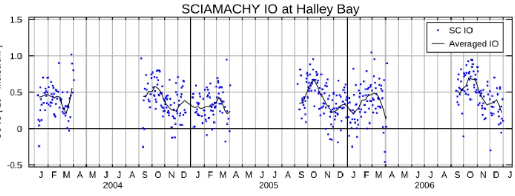
In Fig.6, a time series of IO slant column amounts from SCIAMACHY at Halley is 12973

(17)

ACPD

7, 12959–12999, 2007

Full Screen / Esc

Interactive Discussion shown, covering the three subsequent years from 2004 to 2006. This dataset takes

into account all SCIAMACHY measurements within a square of 500 km side length en-closing Halley Station. Interestingly, the IO time series shows a repeating seasonal pattern. The months without data represent the polar winter periods where scattered sunlight measurements are not possible due to darkness. The maximum in IO values

5

is found for all three years in springtime around October with average values around 7×1012molec/cm2. The amounts decrease but remain positive throughout Antarc-tic summer and rise slightly towards February/March. The increase in AMF due to light path extension during the autumn and spring periods compared to the summer leads to slightly amplified values of IO slant columns from satellite data for these times.

10

However, the change in AMF from spring to summer is at most 15% and does not ex-plain the observed seasonal variation in IO slant column amounts which ranges from 7×1012molec/cm2down to 2×1012molec/cm2in the averaged time series.

This observed pattern compares well with the ground-based LP-DOAS dataset from the CHABLIS campaign. The active LP-DOAS results show IO VMR amounts around

15

3 pptv in Antarctic autumn in March, values close to zero during the dark winter period, then a clear maximum of 7 pptv in the monthly mean in October (with single values up to 20 pptv), and lower but still positive values throughout the Antarctic summer ( Saiz-Lopez et al.,2007a). Consequently, highest values in both, satellite and ground-based measurements are found for the time around October.

20

A direct quantitative comparison between the two measurement types requires an assumption on the vertical distribution of IO. For a constant IO VMR in the lowest 100 m dropping to zero above and a typical value of 4 for the AMF, the maximum in the averaged IO slant column in October, retrieved from satellite measurements corresponds to a VMR of 6–7 pptv, which is in good agreement with the LP-DOAS

25

measurements within the experimental error (Saiz-Lopez et al.,2007a).

For the northern high latitudes, a comparison of IO amounts has also been made with the ground-based MAX-DOAS (multi-axis DOAS) measurements from Ny- ˚Alesund on Spitsbergen (79◦N, 12◦E). Throughout the time when daylight is available,

(18)

ACPD

7, 12959–12999, 2007

Full Screen / Esc

Interactive Discussion tered sunlight spectra are recorded and provide local slant column densities of trace

gases such as IO with some information on the height distribution. The instrumen-tation and retrieval method for the zenith-sky measurements are explained in detail elsewhere (Wittrock et al.,2000,2004). Highest values of IO slant columns detected in Ny- ˚Alesund from MAX-DOAS measurements amount to around 1013molec/cm2for

5

the lowest viewing directions close to the horizon. This converts to values of only 1012molec/cm2for the vertical column, given that the AMF under the prevailing mea-surement conditions is 10 and higher. This value is below the detection limit derived above for the IO column retrieved from a single measurement from SCIAMACHY. Simi-larly, measurements of IO at other locations in the Arctic region have not shown values

10

of IO above the detection limit of around 1 pptv (H ¨onninger et al.,2004).

At locations such as the Irish or Britannic coast, where surface mixing ratios between 0 and 10 pptv of IO have been observed regularly (Peters et al., 2005) the detection limit lies higher compared to areas with high surface reflectivity. According to the es-timations above, IO amounts of around 8 pptv would be detectable at those coastal

15

sites in case the IO is mixed homogeneously over a 1 km thick surface layer and es-pecially, also over the complete area of the satellite ground scene. As the sources of IO at marine sites are spatially and temporally confined, the mean IO column affecting the satellite measurement will fall below the respective detection limit. Additionally, re-cent model studies suggest that the IO is only mixed to lower altitudes on the order of

20

100 m and decreases with height (Saiz-Lopez et al.,2007b). Such a profile leads to a higher surface concentration detection limit for the retrieval of IO from satellite. A cam-paign undertaken by the University of Bremen used the MAX-DOAS instrumentation at the island of Sylt in Northern Germany during May 2005. IO was identified but the daytime values were low with columns being less than or equal to 3×1012molec/cm2

25

(H. Oetjen, yet unpublished results) also below the detection limit for observation from SCIAMACHY.

In agreement with these estimations, no systematically enhanced amounts of IO have been identified over Spitsbergen or European coastal measurement sites in our

(19)

ACPD

7, 12959–12999, 2007

Full Screen / Esc

Interactive Discussion analysis at any time of the year. In conclusion, the limited number of independent

measurements of IO is in reasonable agreement with the magnitude and seasonal behaviour of the IO amounts observed in this study.

8 Discussion

The spatial and seasonal patterns of the IO columns observed from SCIAMACHY, yield

5

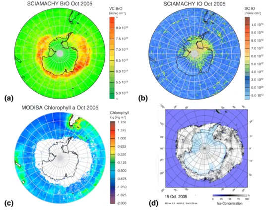
information about the possible sources of IO, in particular when coupled with compar-isons of the amounts and distributions of bromine oxide (BrO), chlorophyll content in the oceans and ice coverage. To compare directly the columns of IO with these other parameters, in Fig.7the southern hemispheric maps of the BrO vertical columns (a), the IO slant columns (b), the chlorophyll concentration in regions of open water (c) and

10

ice coverage (d) for October 2005 are shown.

8.1 IO and ice coverage

It is illuminating to compare the map of IO columns with that for the ice coverage in Antarctica (Fig. 7d). The ice coverage is determined from measurements by the AMSR-E (Advanced Microwave Scanning Radiometer for EOS) instrument onboard

15

the AQUA satellite launched in May 2002, using the 89 GHz channels (Kaleschke et al.,2001;Spreen et al.,2007). The area with enhanced IO amounts is widely extended throughout the Weddell Sea and reaches far over the ice covered area. This supports the proposal that iodine precursors are correlated with or are dependent on condi-tions associated with sea ice at high latitudes. Potential release mechanisms include

20

both the direct release of iodine from the mineral phase and the photolysis of organic iodocarbon compounds, e.g., from the biosphere below and around the sea ice. Either process needs to be particularly effective, as iodine compounds originally come from sea salt, where iodine concentration is fairly small. It should be noted that the retrieval of IO from the SCIAMACHY measurements are intrinsically less sensitive to any IO

25

(20)

ACPD

7, 12959–12999, 2007

Full Screen / Esc

Interactive Discussion present over open water which is not accounted for in the slant columns discussed

here.

8.2 Comparison between BrO and IO values

Enhanced concentrations of BrO are regularly observed over and close to sea ice in polar spring in connection with ozone depletion events and can be observed by satellite

5

(e.g.Richter et al.,1998;Wagner and Platt,1998). Compared to the distribution of BrO in Antarctica, the observations of IO exhibit some similarities but also some interesting and significant differences (Figs.7a, b). In this context, the highest amounts of BrO are found in September, the values remain large throughout springtime and then decrease over the summer with possibly slightly higher amounts of BrO in autumn. This differs

10

from the situation for IO, which has two clear maxima, the first one in October and a second around March.

Likewise, with respect to the spatial distribution of IO and BrO, similarities exist but the behaviours of IO and BrO are also significantly different. While the fact that both IO and BrO appear in the springtime in regions close to one another could be interpreted

15

as indication for similar or even linked release mechanisms, the different spatial pattern found for these two compounds (see Figs. 7a and b) argues for different activation processes for reactive iodine and reactive bromine species. The region where highest BrO amounts are found is of a ring shape above all of the sea ice around the Antarctic continent having varying hot spots. In contrast, the largest IO columns are situated

20

close to and partly overlapping the BrO regions, but they are concentrated further south around the Weddell Sea, along the Antarctic coast, and to some extent in the Ross Sea, including even the shelf ice regions, i.e., the Ross, the Filchner-Ronne and the Amery ice shelves, and also parts of the continent. The higher values above the Antarctic continent and the ice shelves are possibly explained to some extent by

25

transport processes from neighbouring regions. Although in large regions of Antarctica katabatic wind flow prevails, regions with different flow patterns especially in the lowest layers of the atmosphere can still lead to transport of IO or its precursors from sea ice

(21)

ACPD

7, 12959–12999, 2007

Full Screen / Esc

Interactive Discussion regions to the continent. As IO itself is fairly short-lived, transport of related substances,

and especially recycling processes at the snow surface and from the aerosol phase could have an important influence in this respect.

The very cold temperatures above sea ice regions, associated with leads, often re-sult in the formation of frost flowers and such regions of fresh ice have been termed

5

regions of potential frost flower coverage (PFF). The correlation between the source regions of the polar BrO clouds and regions of PFF led to the proposal that bromine is released from brine in aerosols or on freshly formed sea ice and to subsequent dis-cussions (Kaleschke et al.,2004;Piot and von Glasow,2007;R. Sander et al.,2006). The influence of PFF conditions on the release of iodine from cold brine in aerosol or

10

on ice surface is not yet known or studied, but the spatial difference in BrO and IO fields observed indicates that PFF is not as strongly linked to IO as it might be to BrO. Maximum column amounts of BrO of up to 1×1014molec/cm2 are about one order of magnitude higher than that observed for IO. Taking the ratio of bromine to iodine ion concentrations in sea water of [Br]/[I]=15 000 (Wayne,2000) and the removal

pro-15

cesses for BrO and IO into account, any mechanism for iodine release comparable to that described for bromine requires a much more efficient emission of iodine species or a highly iodine selective process. As a consequence, additional pathways are required to explain the release of reactive iodine into the atmosphere over Antarctica. These processes coupled with the local transport need to be distributed widely over the whole

20

region, as the detected IO clouds are not confined to small areas but rather appear to be spread over extended regions. In the following paragraph, the possibility of biogenic pathways is discussed.

8.3 IO and chlorophyll

By analogy with the well-known release of iodine species by macro-algae at

mid-25

latitudinal coastal sites, iodine in the Antarctic is likely to originate at least partly from biological activity. Algae and other biologically active organisms in the cold water and ice have already been identified as a source of emissions of organic iodocarbons (

(22)

ACPD

7, 12959–12999, 2007

Full Screen / Esc

Interactive Discussion penter et al.,2007). The latter are reported to be present in the top layers of Antarctic

water and below the ice, and they are released to the atmosphere by a variety of ex-change processes. It has been shown that dependent on the specific organism, various types of halocarbons are produced in different ratios. As a consequence, the amount of iodinated compounds in the ice and water, and those released to the atmosphere

5

depends amongst other factors on the local biological activity.

The regions of maximum IO amounts in Antarctic spring and autumn are mostly cov-ered with ice, but open water regions and breaking of, or transport through, leaking ice could lead to a flow of gaseous species from the ice, or the underlying water, into the atmosphere. In spite of the low light levels, species such as diatoms multiply in

10

regions partly covered by ice, because it is favourable for them to be attached to the undersurface of the ice cover and the cold ocean water is rich in nutrients. In addition, transfer from organic species within the ice sheets to the atmosphere above is prob-able. Diatoms grow fine underneath multi-year ice, which gets more porous when it ages, and nutrients are still supplied by the currents existing under sea ice.

Consider-15

ing the differences between BrO and IO observations discussed above, IO is located further south also in regions of older sea ice, where therefore the biological pathway could be an explanation for the obtained results.

A useful indicator for biological activity in oceans, directly linked to the occurrence of photosynthesis is the chlorophyll-a pigment concentration (Fig.7c). This is measured,

20

e.g., by the MODIS (Moderate Resolution Imaging Spectroradiometer) instrument on-board the Terra satellite (Barnes et al., 1998; Carder et al., 2004). These data are currently limited to open water regions in the ocean larger than ca. 9 km. This means open water leads and polynya in the ice, smaller than this value are not analysed. Even with a few percent ice within a ground pixel, the reflection from this area exceeds the

25

weak signal reflected from the water that contains the information on chlorophyll con-centration. From the chlorophyll map, it is seen that biological activity is present around the Antarctic. Unfortunately, no data are available for the Weddell Sea and other ice covered regions, preventing any conclusions on possible biogenic sources.

(23)

ACPD

7, 12959–12999, 2007

Full Screen / Esc

Interactive Discussion 8.4 Seasonal variation of IO at southern high latitudes

The availability and amount of precursor substances is one important factor determin-ing the seasonal variation of IO above Antarctica. Another necessary condition for the production of iodine radicals is the availability of sunlight, which photolyses the photo-labile precursor species. As a result, the maximum periods for IO formation represent a

5

concurrence of the conditions of maximum release (and therefore high concentrations) of these precursors, and light levels sufficient for efficient photolysis. Consequently, during winter, IO amounts are expected to be low owing to the lack of actinic flux and low biological productivity. From springtime onwards, when sunlight is available, the precursor substances are photolysed producing the required iodine radicals. Similarly,

10

the growth of algae communities under the ice and the availability of leads and polynya in ice become significant. The decrease in IO amounts during summer time may result from the changing biological activity, associated with the minimum in the sea ice cover. This inference is supported by the observation that organisms and biological activity are distributed over a deeper water column in summer time, whereas they are more

15

concentrated towards the surface facilitating exchange with the atmosphere in spring and autumn (Simpson et al.,2007). Additionally, a second bloom in sea-ice diatoms in Antarctica occurs in autumn, which also supports the explanation that biological path-ways can at least partly cause the seasonal variation observed for IO.

8.5 Other regions

20

Interestingly, no notably enhanced IO amounts have been identified in the Arctic through-out the period analysed in contrast to the situation for BrO. The lower values in the Northern Hemisphere might be explained by the different biological conditions at high latitudes in the Arctic as compared to the Antarctic. Iodocarbons have been found in the Arctic (Schall et al.,1994), but Arctic diatoms are a different species and the production

25

of iodine compounds differs between the various species of algae. The differences in biological activity impacts on the amounts of IO precursors, and the meteorology of

(24)

ACPD

7, 12959–12999, 2007

Full Screen / Esc

Interactive Discussion the Arctic as compared to that around and above Antarctica is likely to lead to different

patterns and amounts of IO for a predominantly biological source.

At mid and low latitudes, the poorer detection limit for the monthly mean IO compos-ites as compared with high latitudes arises from the poorer frequency of measurements and from the lower surface spectral reflectance of oceans as compared to that of ice

5

and snow in the IO spectral window. Consequently, observations of assured columns of IO above the respective detection limit in these regions from satellite measurements are not reported in this study. The observation of enhanced but noisy IO signals above biologically active regions including some up-welling regions such as off the coast of Peru is not further analysed here, but it should be noted nevertheless that this

observa-10

tion would be consistent with the source of IO being the production of iodine containing species by the oceanic biosphere and their direct or subsequent emission to the atmo-sphere.

8.6 Atmospheric significance of the retrieved IO column amounts

With the results from satellite measurements, the significance of iodine oxide in the

15

atmosphere can be estimated. Unless stated otherwise, rate coefficients in this section are taken fromS. P. Sander et al.(2006).

The reaction of I atoms with O₃ initiates a chain reaction removing ozone, which in addition to bromine chemistry contributes to the understanding of the low day-time amounts of tropospheric O₃ observed in the remote marine boundary layer (von

20

Glasow et al.,2002;Dickerson et al.,1999, and references therein).

For the following calculation, the upper limit of 3×1012molec/cm2 in marine areas for the IO vertical column (for AMF=1) and a marine boundary layer of typically 0.5 to 2.5 km height are considered. Assuming that the IO column is confined to a well-mixed marine boundary layer, the upper limit for the concentration will vary in the range

25

below 1 to 6×107molec/cm3 (or 0.4 to 2.4 pptv). This holds in case the IO is evenly distributed on the spatial scale of the SCIAMACHY ground footprint valid here, i.e. 60×120 km2.

(25)

ACPD

7, 12959–12999, 2007

Full Screen / Esc

Interactive Discussion The ratios [Cl]/[ClO], [Br]/[BrO], and [I]/[IO] increase with the size of the halogen

because photolysis of halogen precursors and temporary reservoirs is more effective. Similarly, the tropospheric photolysis frequencies of IO are much larger than that of BrO, which is again larger than that of ClO. Assuming to a first order approximation that I, IO and O₃achieve a stationary state determined by Reactions (R1), (R11) and (R12),

5

the ratio [I]/[IO] would be given by J₍_R11₎/k₍_R1₎[O₃]. With O₃ mixing ratios between 1 to 40 ppbv, the rate coefficient k(R1)=1.2×10−12cm

3

/molec/s at 298 K and J₍_R11₎between 0.03 and 0.24 s−1 (G ´omez Mart´ın et al.,2006;Harwood et al.,1997), the [I]/[IO] ratio lies in the range from 0.025 to 8. This implies that considerable amounts of I atoms might be present under the given conditions. As IO atoms undergo further reactions

10

recovering atomic iodine, such as the self reaction (IO+IO), cross reactions (IO+BrO) and (IO+HO2), ozone will then be catalytically destroyed. The rate of O3loss infered

from this can be compared to the O₃ destruction through bromine chemistry. The approximated loss rates are given by k₍_R1₎[I][O₃] for the iodine cycle and in analogy k₍_R1₎[Br][O₃] for the bromine cycle, where the reaction rates (k₍_R1₎) of the two halogens

15

with ozone take on the same value. The [Br]/[BrO] ratio is smaller than the [I]/[IO] ratio by typically one order of magnitude. In model studies byVogt et al.(1999), the ratio [Br]/[BrO] lies around 0.035–0.07 in a base run, while [I]/[IO] from the above estimate yields a ratio of 0.35 if the same atmospheric conditions as in that model run are applied. This means that even if BrO amounts are higher than IO amounts by one

20

order of magnitude, the O₃loss rates can lie in the same range. In comparison, model studies byvon Glasow et al.(2002) infer that the presence of small amounts of iodine increases tropospheric ozone loss by up to 40%.

The potential for particle formation in the marine boundary layer by iodine chemistry needs to be addressed. Higher iodine oxides, which can form adducts with water, and

25

iodine oxide clusters act as condensation nuclei for aerosol formation. As the rate of higher oxide production depends on the square of the IO concentration, this is a highly non-linear process. The upper limit for the rate of particle formation R(I-aerosol) is given by the rate of higher oxide formation, i.e. R(I-aerosol)≈(k(R13)+k(R14))[IO]2.

(26)

ACPD

7, 12959–12999, 2007

Full Screen / Esc

Interactive Discussion For comparison, the formation of particles from sulphur species can be estimated.

The average rate of formation of H₂SO₄ is determined by the rate of the three body reaction (R17) of OH with SO₂, as the reaction rates of Reactions (R18) and (R19) are rapid under the conditions of the marine boundary layer.

OH + SO2+ M → HOSO2+ M (R17)

HOSO₂+ O2→ SO3+ HO2 (R18)

SO₃+ H2O → H2SO4 (R19)

The following assumptions are made: k₍_R17₎ has reached its high pressure limit of k₍_R17₎≈1.6×10−12cm3/molec/s, the background marine boundary layer has of the or-der of 100 pptv of SO₂ from dimethyl sulphide, CH₃SCH₃ (DMS), and the daytime concentration of OH is approximately 1×106molec/cm3.

The rate of removal of SO₂by OH in the remote boundary layer (followed by

forma-5

tion of aerosol) is determined by the rate of (R17)≈R(S-aerosol)≈k(R17)[OH][SO2] and

can be compared to the rate of formation of the higher iodine oxides (R13,R14), for the given assumptions. With k_IO+IO=8×10−11cm3/molec/s and (k₍_R13₎+k(R14))/kIO+IOclose

to 1 (Bloss et al.,2001), the ratio of these rates, R(I-aerosol)/R(S-aerosol) varies be-tween (<2 to 72). Possibly, iodine could be a significant source of atmospheric aerosol

10

in the remote marine boundary layer in addition to that from the oxidation of sulphur. In this context, it is already known that iodine chemistry is a significant local source of new particles (O’Dowd and Hoffmann,2005;McFiggans et al.,2004). Detailed models, taking into account the non-linearity of the iodine and sulphur chemistry and including accurate estimates of the release of DMS and iodine atom precursors, are required

15

to assess accurately the relative importance of iodine chemistry as a global source of particles.

(27)

ACPD

7, 12959–12999, 2007

Full Screen / Esc

9 Summary and conclusions

Using nadir measurements from the SCIAMACHY satellite instrument, global maps of the IO column density were retrieved for the years 2004 to 2006, with a focus on 2005, by means of the DOAS retrieval method. The theoretical detection limit of a few 1012molec/cm2 lies close to the expected IO amounts observed thus far by

ground-5

based measurements. For a given VMR in the ground layer, the applicability of satellite measurements for IO columns strongly depends on surface spectral reflectance of the ground scene and the height to which IO is mixed, i.e. the vertical profile of IO, in the atmosphere. However, in regions of enhanced IO amounts and high surface reflectivity, the unambiguous detection of IO with SCIAMACHY is possible.

10

Close to Antarctica, large areas, exhibiting IO amounts considerably above the de-tection limit for the retrieval of IO columns from SCIAMACHY, have been identified from spring to autumn. The highest monthly average values of IO slant columns are found for October and March (springtime and autumn) close to the Antarctic continent, espe-cially in the Weddell Sea, and amount up to 8×1012molec/cm2, while values on single

15

days can be significantly higher.

A seasonal variation of IO columns in the Antarctic region is revealed, in which the IO columns show generally low values in winter, as far as these regions are accessi-ble to satellite measurements, a maximum during springtime, decreasing values during summer and a second peak in Antarctic autumn. This seasonal pattern is confirmed by

20

a long-term time series of three years of data around Halley Station, Antarctica, where this same behaviour is repeated every year. Comparing this time series of satellite ob-servations to ground-based measurements at Halley (Saiz-Lopez et al.,2007a), good agreement is achieved within the respective error limits for this seasonal evolution of IO amounts. No enhanced amounts of IO could be seen for the Arctic region

through-25

out the period analysed, indicating some systematic differences in the availability of precursor substances between the northern and southern hemispheric polar regions.

Ice cover maps show that positive detection of IO reaches over large ice covered

(28)

ACPD

7, 12959–12999, 2007

Full Screen / Esc

Interactive Discussion areas in Antarctica, revealing some correlation of enhanced IO amounts with ice

cov-erage and supporting the connection of ice to the release of reactive iodine. This implies that direct abiotic and/or biogenic sources of iodine are probably associated with the ice sheets.

The comparison between IO and BrO maps reveals differences in the spatial and

5

temporal distribution of these two halogen oxides. Some similarities such as the oc-currence of IO and BrO maxima in the Antarctic springtime support the concept that chemistries of these halogen oxides are to some extent coupled and may have some common sources, but the differences in the patterns provide evidence that significantly different sources of bromine and iodine are required. These findings for the IO

distribu-10

tions are interpreted as indicating the existence of a biological source of iodocarbons and possibly I₂, which act as precursors of reactive iodine. Chlorophyll maps from MODIS give an indication of biological activity in open water regions, but the smaller open water leads and activity under the ice are not determined.

Sufficient solar actinic irradiation for the photolysis of the iodine containing species

15

in the boundary layer represents another necessary condition for the production of IO. This condition explains part of the observed seasonality of IO at high latitudes. Sea-sonal variations of the not yet fully identified release processes are needed to complete and enhance our understanding in the future. For a more conclusive interpretation of IO more detailed information on the biological situation, emission properties of the sea

20

ice layers and the chemical cycles involved are needed. Similarly, modelling of the complex iodine and sulphur chemistry of the remote marine boundary is necessary to assess accurately the magnitude of the catalytic loss of O₃and the number density of particles originating from the chemistry of iodine. However, the magnitude and distri-bution of the IO columns observed in this study indicates that both of these processes

25

could be of potential local and even global significance for tropospheric chemistry.

Acknowledgements. This study has been supported by the State and University of Bremen,

the German Aerospace (DLR), and the European Union. ESA and the DLR kindly provided the level 1 data from SCIAMACHY used in this study. We would like to thank the British Antarctic

(29)

ACPD

7, 12959–12999, 2007

Full Screen / Esc

Survey, the NERC and especially A. Saiz-Lopez and J. M. C. Plane for the provision of ground-based data from the CHABLIS campaign. Chlorophyll-a data from MODIS was kindly provided by NASA/GSFC. We also would like to thank L. Kaleschke for helpful discussions and provision of ice maps.

References

5

Alicke, B., Hebestreit, K., Stutz, J., and Platt, U.: Iodine oxide in the marine boundary layer, Nature, 397–398, 572, 1999. 12960,12961

Allan, B. J., McFiggans, G., Plane, J. M. C., and Coe, H.: Observations of iodine monoxide in the remote marine boundary layer, J. Geophys. Res., 105, 14 363–14 369, 2000. 12961,

12962

10

Barnes, W. L., Pagano, T. S., and Salomonson, V. V.: Prelaunch characteristics of the Mod-erate Resolution Imaging Spectroradiometer (MODIS) on EOS-AM1, IEEE Transactions on Geoscience and Remote Sensing, 36(4), 1088–1100, 1998.12979

Barrie, L. A., Bottenheim, J. W., Schnell, R. C., Crutzen P. J., and Rasmussen, R. A.: Ozone destruction and photochemical reactions at polar sunrise in the lower Arctic atmosphere, 15

Nature, 334, 138–141, 1988. 12963,12964

Bloss, W. J., Rowley, D. M., Cox, R. A., and Jones, R. L.: Kinetics and Products of the IO Self-Reaction, J. Phys. Chem. A, 105, 7840–7854, 2001. 12964,12983

Bogumil, K., Orphal, J., Homann, T., Voigt, S., Spietz, P., Fleischmann, O. C., Vogel, A., Hartmann, M., Bovensmann, H., Frerik, J., and Burrows, J. P.: Measurements of Molecu-20

lar Absorption Spectra with the SCIAMACHY Pre-Flight Model: Instrument Characterization and Reference Data for Atmospheric Remote-Sensing in the 230–2380 nm Region, J. Pho-tochem. Photobiol. A., 157, 167–184, 2003. 12968

B ¨osch, H., Camy-Peyret, C., Chipperfield, M. P., Fitzenberger, R., Harder, H., Platt, U., and Pfeilsticker, K.: Upper limits of stratospheric IO and OIO inferred from center-25

to-limb-darkening-corrected balloon-borne solar occultation visible spectra: Implications for total gaseous iodine and stratospheric ozone, J. Geophys. Res., 108(D15), 4455, doi:10.1029/2002JD003078, 2003. 12962

Bovensmann, H., Burrows, J. P., Buchwitz, M., Frerick, J., No ¨el, S., Rozanov, V. V., Chance,