HAL Id: hal-00811223
https://hal.archives-ouvertes.fr/hal-00811223
Submitted on 23 Apr 2012
HAL is a multi-disciplinary open access
archive for the deposit and dissemination of
sci-entific research documents, whether they are
pub-lished or not. The documents may come from
teaching and research institutions in France or
abroad, or from public or private research centers.
L’archive ouverte pluridisciplinaire HAL, est
destinée au dépôt et à la diffusion de documents
scientifiques de niveau recherche, publiés ou non,
émanant des établissements d’enseignement et de
recherche français ou étrangers, des laboratoires
publics ou privés.
Interpolation of room impulse responses in 3d using
compressed sensing
Rémi Mignot, Laurent Daudet, Francois Ollivier
To cite this version:
Rémi Mignot, Laurent Daudet, Francois Ollivier. Interpolation of room impulse responses in 3d using
compressed sensing. Acoustics 2012, Apr 2012, Nantes, France. �hal-00811223�
Interpolation of room impulse responses in 3d using
compressed sensing
R. Mignot
a, L. Daudet
aand F. Ollivier
ba
Institut Langevin “ Ondes et Images ””, 10 rue Vauquelin, 75005 Paris, France
b
UPMC - Institut Jean Le Rond d’Alembert, 2 place de la gare de ceinture, 78210 Saint Cyr
L’Ecole, France
In a room, the acoustic transfer between a source and a receiver is described by the so-called “Room Impulse Response”, which depends on both positions and the room characteristics. According to the sampling theorem, directly measuring the full set of acoustic impulse responses within a 3D-space domain would require an unrea-sonably large number of measurements. Nevertheless, considering that the acoustic wavefield is sparse in some dictionaries, the Compressed Sensing framework allows the recovery of the full wavefield with a reduced set of measurements (microphones), but raises challenging computational and memory issues. In this paper, we exhibit two sparsity assumptions of the wavefield and we derive two practical algorithms for the wavefield estimation. The first one takes advantage of the Modal Theory for the sampling of the Room Impulse Responses in low fre-quencies (sparsity in frequency), and the second one exploits the Image Source Method for the interpolation of the early reflections (sparsity in time). These two complementary approaches are validated both by numerical and experimental measurements using a 120-microphone 3D array, and results are given as a function of the number of microphones.
1
Introduction
The acoustic properties of a reverberating room can be given by analysing its Room Impulse Responses (RIRs). In [1], the concept of Plenacoustic Function (PAF) is intro-duced. This function gathers all RIRs of the room, and thefore it depends on time, on the source position, on the re-ceiver position and on the room characteristics (geometry and wall properties).
On one hand, in some applications the effect of room re-verberation is undesirable and acoustic echo cancelers are used to estimate the anechoic sound. On the other hand, re-verberation plays an important role in auditory scene synthe-sis, in virtual reality framework for example. In both cases, knowing the whole set of RIRs in a given room could poten-tially be used to improve their performance.
Measuring the PAF is fundamentally a sampling problem: from a limited number of point measurements, the goal is to reconstruct (i.e. interpolate) the acoustic wavefield at any position in space and at any time.
1.1
Sampling of the Plenacoustic Function
Standard acquisition of signals relies on a regular sam-pling of space and time with respect to Shannon-Nyquist the-ory. Basically, to sample a band limited signal between 0 and fc [Hz], the sampling rate Fshas to be chosen higher than
2 fc. In the same way, the space sampling has to be dense
enough to avoid aliasing in reconstruction.
Considering a fixe source and a 3-D regular microphone array, the Nyquist criterion is satisfied if (cf. [1]):
δv<
c0
2 fc
, ∀v ∈ {x, y, z} , (1)
where δx, δyand δz are the sampling steps along the 3 axes.
Physically, this criterion states that the sampling steps must be smaller that the half of the minimal wavelength λ=c0/ fc.
Unfortunately, the measurement of a time varying 3-D image requires a too high number of microphones to be real-ized as such in practice. For example, in order to reconstruct the PAF inside a cube with side 2 m, and with fc = 6 kHz,
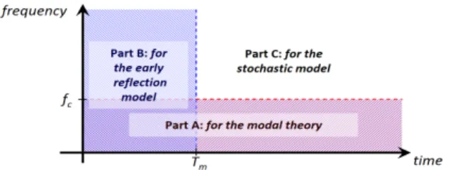
we need at least 340.103point measurements (microphones). Nevertheless, in [2] it is shown that the RIR part above a certain Schroeder frequency (cf. [3]) and after a certain mix-ing time(cf. [4]) behaves like a colored, modulated noise and can be modeled and simulated using a stochastic model (part C in fig. 1). Consequently, to reduce the number of required microphones, we propose to sample only the hatched part of fig. 1. For example, in [5] the low frequencies of the RIRs
Figure 1: Validity parts of the models. Here fcand Tmare
associated to the Schroeder frequency and the mixing time respectively
(part A) are reconstructed using a model based on the modal theory, and in [6] a method based on Dynamic Time Warp-ing is proposed for the interpolation of the early part of the RIRs (part B). But these 2 methods have been developped for the interpolation of the RIRs on a line, and here we want to sample the PAF in a 3-D domain.
In this work, we propose a method to sample and to inter-polate in 3-D the parts A and B separately (cf. fig. 1), using the same measurements. In order to reduce the number of microphone in the array, an interesting approach is the Com-pressed Sensingframework which is briefly described below.
1.2
Compressed Sensing
The problem consists in the reconstruction of a signal y ∈ RN from M observations x
m, linked by the linear
sys-tem x= Φy. Compressed Sensing (CS) deals with the under-determined case, for which there are more unknowns than equations (N > M), cf. e.g. [7, 8]. As such a problem cannot be solved without additional hypothesis, the underlying idea is that if y lives in a subspace of dimension K and with basis ψ, for K < M, we can solve y = ψa writing x = Φy = Φψa = θa. But, in general we do not know ψ.
Then, we define L vectors ψl, forming the matrixΨ with
L K, and we look for a basis which explains y. In other words, we look for a vector α ∈ RLK-sparse (where no more
than K coefficients are non-zero), such that y = Ψα. Un-fortunately this problem is not convex and difficult to solve. However, we can change it into a convex problem by consid-ering the following Basis Pursuit Denoising approach:
min
α∈RLkαk`1 subject to kx −ΦΨαk`2
≤ε, (2)
where the norm `nis given by kyk`n = (Pi|yi|n)1/n, and ε is a
fidelity parameter. A high ε allows a stronger sparsity of α, and a small ε improves the reconstruction of y.
Some theoretical results (cf. e.g. [9, 10]) give a sufficient condition for reconstructing y in the case of sparse signals,
by the so-called Restricted Isometry Property (RIP). It quan-tifies howΦ and Ψ are mutually incoherent with respect to their use on sparse signals. In practice, the RIP is difficult to compute, but it is verified with high probability for some random sampling matrices. This encourages the use of ran-domly selected observation points in practice, which are here the microphone positions in the 3-D space.
In this work we will consider the Modal Theory and the Image Source Methodin order to justify the use of CS for the parts A and B respectively (cf. fig. 1). We will see that these 2 deterministic models give 2 sparse representations of the PAF in their respective part: sparsity in frequency for part A, and sparsity in time for part B.
1.3
Outline
The outline of this paper is as follows. In section 2, con-sidering two acoustic models consecutively, we show that the two parts of the PAF (low frequencies and early reflections) can have a sparse representation in some respective dictio-naries, and so that the Compressed Sensing framework can be used. For these two models, we briefly present the de-rived algorithms of decomposition. Then, in section 3, we present some experimental results and some comparisons. Note that this paper focuses on the experimental results of the proposed approaches, for more details about the algorithms, see [11, 12]. Finally, in section 4, we conclude this paper.
2
Modelling and CS algorithms
2.1
Modal Theory
Here, we proposed two methods based on the modal the-ory for the interpolation of the PAF in low frequencies. 2.1.1 Structured Sparsity
Considering linear acoustic propagation away from the sources, the acoustic pressure p(t, ~X) is governed by the wave equation c02∆p(t, ~X) − ∂2tp(t, ~X) = 0, where ∆ = ∇2 is the
laplacian operator and ∂tis the time derivative. Assuming a
modal behavior (at low frequencies) for closed rooms with ideally rigid walls, the solution can be decomposed as a dis-crete sum of complex harmonic signals with the angular fre-quencies ωq:
p(t, ~X)= X
q∈Z?
Aqφq( ~X) gq(t), (3)
where gq(t)= ejωqt, φqis the modal shape of the mode q and
Aq is a related complex amplitude. With the wavenumber
kq = ωq/c0, we get the Helmholtz equation for every mode:
∆φq+ kq2φq= 0.
In the Helmholtz equation, φq is the eigenmode of the
laplacian operator with eigenvalue −k2q. If the room is
star-shaped, previous studies [13, 14] have shown that an eigen-mode of the laplacian with a negative eigenvalue can be ap-proximated by a finite sum of plane waves incoming from various directions, and sharing the same wavenumber kq. Then
φq( ~X) ≈ R
X
r=1
aq,rej~kq,r~X (4)
is the R-order approximation of φq, with ~kq,rthe 3-D
wavevec-tor r of the mode q, such that k~kq,rk2= |kq|.
In the case of non rigid walls, the modes are damped in time, kqnow has an imaginary part: kq= (ωq− jξq)/c0, where
ξq < 0 is the damping coefficient. Therefore, gq(t) of eq. (3)
becomes: gq(t) = ejkqc0t = eξqtejωqt. In theory, these losses
modify φq, nevertheless we assume that the approximation
(4) remains valid, at least for ~Xfar from the walls.
Consequently, considering a finite frequency range [0, ωc]
containing Q real modes, or equivalently 2Q complex modes, and considering R-order approximations of the φq’s, the PAF
p(t, ~X) can be approximated by a sum of 2QR damped har-monic plane waves, exp( j(kqc0t+ ~kq,r~X)).
Now, taking advantage of this Structured Sparsity, and starting from the sampled signals p(tn, ~Xm) of a array of M
microphones at ~Xmcovering a 3-D domain of interestΩ (a
finite convex domain within the room), we present an algo-rithm previously proposed for the near-field acoustic holog-raphy of plates [15]:
(a) The shared wavenumbers kqare estimated using a joint
estimation of damped sinusoidal components (cf. [16]). (b) The operational shapes φq of (3) are estimated using
the projection of the measured signal onto a basis for-med by the damped exponentials ejkqc0t.
(c) Every φqis approximated using a finite sum of plane
waves sharing the same wavenumber kq(cf. eq. (4)).
(d) Finally, the PAF can be interpolated ∀t ∈ [0, N/F s] and ∀ ~X ∈Ω using ˜p(t, ~X) = Pqα˜q,rej(kqc0t+~kq,r~X), where
˜
αq,rare the coefficients optimised in stage (c).
2.1.2 Modal analysis in a rectangular room
In this section, we study the solutions of the wave equa-tion in the simple case of a rectangular room. From this study, we exhibit a stronger property of sparsity which justi-fies the use of the Compressed Sensing framework (CS).
In the case of a rectangular room with rigid walls, we can make the variable separation in cartesian coordinates (x, y, z). Then, each modal shape is written as the product of 3 func-tions of one variable. With ~X= [x, y, z]T, the PAF becomes:
p(t, ~X)=X
q∈Z?
AqFxq(x) Fyq(y) Fzq(z) ejkqc0t. (5)
For each mode, these functions verify the 1-D Helmholtz equation ∂2
vFv+ k2vFv = 0 for v ∈ {x, y, z}. With rigid walls,
the kv’s are real constants such that k2x+k 2 y+k
2 z = k
2(cf. [17]).
According to the Helmholtz equation, for each cartesian co-ordinate v the Fv’s are the sum of 2 solutions: Fv(v)= A+ve
jkvv
+A−
ve− jkvv. Then, expanding FxFyFz, the modal shape φq( ~X)
is written as the sum of 8 plane waves e± jkxx± jkyy± jkzz= ej~k ~X,
with ~k= [±kx, ±ky, ±kz]T.
In the case of non rigid walls, as the wavenumber k is complex: k= (ω − jξ)/c0, the kv’s are complex. This implies
a slight decrease of the Fv’s near the walls. Nevertheless, for
~X far from the walls, we assume that the imaginary part of kv
is negligible, and that k2
x+ k2y+ k2z = Re(k)2= ω2/c02.
Consequently, in a bandwidth containing 2Q complex mo-des, the PAF can be written as the sum of 16Q harmonic plane waves in the case of rectangular rooms. Note that in
the previous section, each modal shape was approximated by R fixed plane waves sampling uniformly the sphere of ra-dius |ω|/c0, whereas here, with the assumption of rectangular
room, only 8 plane waves are required by complex mode. In this work, the proposed method is based on the Match-ing Pursuitalgorithm (cf. e.g. [18]). It consists in iteratively substracting from the signal the group of 8 harmonic planes waves exp( j(kt+ ~k~X)) that best approximates the measured PAF. These plane waves are associated to one mode and share the same wavenumber k.
Although this model doesn’t hold for arbitrary geome-tries (cylindrical rooms for example), it can nevertheless be extended to non rectangular rooms. Indeed, if all walls are plane, we can assume that the modal shapes are still sparse on a dictionary of plane waves. The corresponding wavevec-tors remain on the sphere of radius |k|.
2.2
Image Source Method
The principle of the Image Source Method is that an acous-tic path involving reflections in an enclosed space can be represented by a straight line path connecting the listener to a corresponding Virtual Source (VS) emitting in free space. For a fixed real source at position ~Y0and a receiver at position
~X, the RIR have the general form (cf. e.g. [19]): p(t, ~X)=X s∈J βs δ(t − k~X − ~Ysk2/ c0) 4π k ~X − ~Ysk2 , (6)
where the ~Ys are the VSs positions, the βs coefficients take
into account the damping caused by the multiple reflections against the walls, and J is a set indexing the virtual sources. For the early part t ∈ [0, T ] of the RIRs, we only have to take into account the VSs within a ball of radius r= T c0
and center ~X. As a consequence, since the RIRs are repre-sented as linear combinations of contributions of a few VSs (cf. eq. (6)), the early part of the 4 dimensional function p(t, ~X) has a sparse representation on a dictionary of spher-ical waves, where the centers are the VSs. Then, to recon-struct p(t, ~X) in a finite time interval [0, T ] and in a domain Ω of the space, we propose to exploit this sparsity using the CS approach.
As in section 2.1, the present method is based on the Matching Pursuit algorithm (cf. e.g. [18]). Here, it itera-tively substracts from the measured PAF the atom that best approximates it. This atom is chosen among a dictionaryΨ of monopoles within a virtual space which is a ball of radius r = Tc0 and of center the microphone array. Then, every
atom ψsofΨ is given by
ψs[n, m]=
δ(tn− k ~Xm− ~Ysk2/ c0)
4π k ~Xm− ~Ysk2
. (7)
The underlying assumptions of this model are as follows: the walls have to be plane, only specular reflections are con-sidered (no diffuse reflections), diffraction is not taken into account, the domainΩ of analysis and reconstruction has to be small enough in order to avoid a problem of visibility of the VSs according to ~X(cf. [19]), and the imaginary part of the wall reflections (in the frequency domain) have to be suf-ficiently small. Note that for convex rooms, diffraction can be neglected, and we consider complex wall reflections for a more realistic modeling (cf. [12] for more details).
3
Experiments and results
We have designed a real 3-D array with 120 electret mi-crophones (cf. fig. 2), randomly positioned within a cube of size 2m with a statistical distribution close to uniform - up to mechanical constraints. The room has dimensions (3.8, 8.15, 3.6)m, it was emptied but still had features that made it non-ideal: a doorway, two windows, a cornice, concrete walls, wood panels, etc.
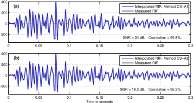
Figure 2: Photograph of the experimental microphone array Here, we present some results of the proposed algorithms, using the same experiment. They will be named: methods CS-A1and CS-A2 for the reconstruction in low frequencies (cf. sec. 2.1.1 and 2.1.2 respectively), and method CS-B for the reconstruction of the early part (cf. sec. 2.2). Interpola-tion CS-A1 and CS-A2 are compared using the estimaInterpola-tion of their Signal-to-Noise Ratio (SNR) [dB], and method CS-B is evaluated using its SNR and its Pearson correlation coef-ficient c [%]. With s the (N × 1) vector of the target RIR, such that s[n] = p(tn, ~X), andes its interpolation: SNR = 20 log (ksk2/ ks −esk2) and c= 100 |hs,esi|/ (ksk2. kesk2).
0 0.05 0.1 0.15 0.2 0.25 0.3 −200 0 200 400 SNR = 24 dB, Correlation = 99.8%. Interpolated RIR, Method CS−A1 Measured RIR 0 0.05 0.1 0.15 0.2 0.25 0.3 −200 0 200 400 Time in seconds SNR = 18.2 dB, Correlation = 99.2%. Interpolated RIR, Method CS−A2 Measured RIR
(a)
(b)
Figure 3: Methods CS-Ax. Example of two interpolated responses in low frequencies: fc= 300 Hz
0 0.005 0.01 0.015 0.02 0.025 −1000 0 1000 −1000 0 1000 SNR = 7.14 dB, Correlation = 90.3%. Time in seconds Measured RIR Interpolated RIR
Figure 4: Method CS-B. Example of the interpolation of the early part
Figures 3 and 4 present some examples of the interpo-lated RIRs, togehter with the measured ones. The analysis is performed using 119 microphones of the array, and the interpolations are evaluated using the measured RIR of the 120th microphone. Remark 1: as opposed to fig. 4, in fig. 3 the contributions of the reflections are not distinguishable be-cause of the low-pass filtering at 300Hz. Remark 2: the RIR of fig. 4 takes into account the non-ideal responses of the microphones and the loudspeaker. Remark 3: whereas the SNRs of methods CS-A1 and CS-A2 are quite good (24dB and 18.2dB respectively), the SNR of method CS-B doesn’t seem as good (7.14dB). But we can remark that the corre-lation remains quite good (90.3%). This point will be dis-cussed in conclusion.
In figure 5, the performances are evaluated according to the number of microphones for the analysis. Here, we have randomly selected 15 microphones for the interpolation and the SNR averages, and the analyses are performed using the 105 other microphones. As a general trend, performance de-creases with M. It is however interesting to notice that with M > 40 method CS-A1 outperfoms method CS-A2 which suddenly falls for M < 16. Nevertheless, between 19 and 28 microphones method CS-A2 is better with a stable SNR (ap-proximately 10dB); this observation has been noticed with other tests. 12 16 19 23 28 34 40 46 52 60 70 80 92 105 −5 0 5 10 15 20 25
M (number of microphones for the analysis)
Signal−to−Noise Ratio [dB] Method CS−A1 Method CS−A2 12 16 19 23 28 34 40 46 52 60 70 80 92 105 0 2 4 6 8
M (number of microphones for the analysis)
Signal−to−Noise Ratio [dB] 12 16 19 23 28 34 40 46 52 60 70 80 92 105 76 82 88 94 100Pearson Correlation [%] SNR [dB] Correlation [%]
Figure 5: Effect of the number of microphones for the analysis. Top: Methods CS-Ax, bottom: Method CS-B
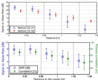
Figure 6 presents the performances according to the dis-tance of the interpolation position from the center of the ar-ray. In this figure, the vertical lines represent the standard deviation of the SNRs per interval. As expected, the per-formances decrease when the position moves away from the center, although it can be noticed that whereas method CS-A1 is better around the center of the array, the SNR of method CS-A2 decreases slower and is better at the edge.
An interesting experiment is the comparison of the meth-ods according to the array configuration. In figure 7, we have numerically simulated and tested 6 different array configura-tions with 125 microphones: 3 random arrays (with a uni-form distribution within the cube with side 2m), the exper-imental array (which is approximately random, cf. fig. 2), a spherical array with radius 1.24m (for which the volume is 8m3like the cube), and a regular array (where the receivers
are uniformly positioned within the cube with side 2m). The noticeable result is that: whereas methods A1 and CS-A2 (for low frequencies) are better with random arrays, as expected, the best result for method CS-B (early part) is
ob-0 0.33 0.66 1 1.33 1.66 −10 −5 0 5 10 15 20 25 30 Distance [m] Signal−to−Noise Ratio [dB] Method CS−A1 Method CS−A2 0 0.33 0.66 1 1.33 1.66 2 4 6 8 10
Distance to the center [m]
Signal−to−Noise Ratio [dB] 0 0.33 0.66 1 1.33 1.66 80 85 90 95 100 Pearson Correlation [%] SNR [dB] Correlation [%]
Figure 6: Effect of the distance from the array center. Top: Methods CS-Ax, bottom: Method CS-B
tained with the regular array. The first observation can be ex-plained because for Compressed Sensing, the measured sig-nals have to be decorrelated from the decomposition dictio-nary (plane waves), consequently random arrays are prefer-able (cf. the RIP property in sec. 1.2) . Moreover with ran-dom arrays, the probability that all microphones lie on the zeroes of a modal shape is smaller than with regular arrays. For method CS-B (for early reflections), the observation can be explained because the diffences of time of arrival have to be maximized between the microphones of the array, and this is done with a regular array where the microphones are uniformly spaced. Nevertheless, we have realised a random array because method CS-B remains acceptable, and because method CS-A1 cannot be used with regular array.
Array (rd1) Array (rd2) Array (rd3) Array (xp) Array (sp) Array (cb) 0 5 10 15 20 25 30 Array configuration Signal−to−Noise Ratio [dB] Method CS−A1 Method CS−A2
Array (rd1) Array (rd2) Array (rd3) Array (xp) Array (sp) Array (cb)
10 12 14 16 18 20 Array configuration Signal−to−Noise Ratio [dB]
Array (rd1) Array (rd2) Array (rd3) Array (xp) Array (sp) Array (cb) 95
96 97 98 99 100 Pearson Correlation [%] SNR [dB] Correlation [%]
Figure 7: Six different microphone arrays. Top: Methods CS-Ax, bottom: Method CS-B
We have checked the robustness of both methods to the geometry of the room, in particular when the measured room gets further away from the “ideal” rectangular room. This has been made by opening the windows and the door, and by placing a chair and a wood panel. Moreover, in the first set of experiments the baffled loudspeaker, which has a complex directivity pattern, was oriented towards the array ; in this second set of experiments the loudspeaker was turned so as to not face the array. The results of these new measurements reveal that methods CS-A1 and CS-A2 (based on the modal
theory) are stable with obstacles and with several orientations of the loudspeaker, while the SNR for method CS-B (based the image source method) decreases.
For methods CS-A1 and CS-A2, since the modal density strongly increases with the frequency, the sparsity assump-tion is less and less valid in high frequencies. Indeed, the performances of method CS-A1 decreases when the cutoff frequency fcincreases, but method CS-A2 seems very stable
when fcvaries, at least up to 400Hz.
In the same line for method CS-B, since the echo density strongly increases with time, the sparsity assumption is less and less valid. Indeed, when the RIRs duration increases for the analysis, the global performance decreases. Nevertheless, we observe that the interpolation quality doesn’t change at the begining of the reconstructed response.
4
Conclusion
Starting from a random array with a small number of mi-crophones, and exploiting two sparsity assumptions of the acoustic wavefield in reverberating room (sparsity in frequen-cy and sparsity in time), we have shown that it is possible to use the Compressed Sensing framework to interpolate in space the Room Impulse Responses. Consequently, we can seperately sample the low frequencies and the early reflec-tions of the Plenacoustic Function (respectively part A and part B of fig. 1), but using the same measures. Then, part C can be synthesized using a stochastic model (cf. [2]).
Note that, the performances are evaluated using the SNR and the correlation coefficient which are probably not signif-icant. For specific applications, more relevant criteria should be designed. For example human perception should be taken into account in the case of a digital reverberation.
Acknowledgments
The authors want to thank Dominique Busquet and Chris-tian Ollivon, for their precious help in the realisation of the microphone array and the acquisition of the RIRs.
References
[1] T. Ajdler, L. Sbaiz, M. Vetterli, “The Plenacoustic Function and its Sampling”, IEEE Transaction on Sig-nal Processing, p. 3790-3804 (2006)
[2] J.-M. Jot, L. Cerveau, O. Warusfel, “Analysis and Syn-thesis of Room Reverberation Based on a Statistical Time-Frequency Model”, AES 103rd Conv., (1997) [3] M. Schroeder, “Statistical parameters of the frequency
response curves of large rooms”, Journal of the AES, p. 299-306 (1987).
[4] J.-D. Polack, “Playing billard in the concert hall: the mathematical foundations of geometrical room acous-tics”, Applied Acoustics, 38 p. 235-244 (1993). [5] Y. Haneda, Y. Kaneda, N. Kitawaki,
“Common-Acoustical-Pole and Residue Model and Its Application to Spatial Interpolation andExtrapolation of a Room Transfer Function”, IEEE Trans. on Speech and Audio Proc., p. 709-717 (1999)
[6] C. Masterson, G. Kearney, F. Boland, “Acoustic Im-pulse Response Interpolation for Multichannel Systems using Dynamic Time Warping”, AES 35th Conf. (2009) [7] E. Cand`es, M. Wakin, “An introduction to compressive
sampling”, IEEE Sig. Proc. Mag., p. 21-30 (2008) [8] R. Baraniuk, “Compressive sensing”, IEEE Sig. Proc.
Mag., p. 118-121 (2007)
[9] E. Cand`es, “Compressive sampling”, International Congress of Mathematicians, (2006)
[10] E. Cand`es, T. Tao, “Decoding by linear programming”, IEEE Trans. on Inform. Theory, p. 4206-4215 (2005) [11] R. Mignot, G. Chardon, L. Daudet,
“Compres-sively sampling the plenacoustic function”, SPIE Conf. Wavelets and Sparsity XIV, vol. 8138 08, (2011). [12] R. Mignot, L. Daudet, F. Ollivier, “Compressed sensing
for acoustic response reconstruction: interpolation of the early part”, IEEE WASPAA’11, p. 225-228 (2011) [13] E. Perrey-Debain, “Plane wave decomposition in the
unit disc: Convergence estimates and computational as-pects”, J. Comp. App. Math., p. 140-156 (2006) [14] A. Moiola, R. Hiptmair, I. Perugia, “Approximation by
plane waves”, Research Report (ETH Z¨urich), (2009) [15] G. Chardon, A. Leblanc, L. Daudet, “Plate impulse
response spatial interpolation with sub-Nyquist sam-pling”, JSV, p. 5678-5689 (2011)
[16] G. Chardon, L. Daudet, “Optimal Subsampling of Mul-tichannel Damped Sinusoids”, 6th IEEE SAM, (2010) [17] H. Kuttruff, “Room Acoustics”, Spon press (2000) [18] M. Elad “Sparse and Redundant Representations: From
Theory to Applications in Signal and Image Process-ing”, Springer, (2010)
[19] J. Borish, “Extension of the image model to arbitrary polyhedra”, JASA, p. 1827-1836 (1984)