Arctic, Antarctic, and Alpine Research, Vol. 49, No. 3, 2017, pp. 411–425 DOI: http://dx.doi.org/10.1657/AAAR0016-049
Open Access – This work is licensed under a Creative Commons Attribution 4.0 (CC BY 4.0) International license.
Three decades of volume change of a small Greenlandic glacier
using ground penetrating radar, Structure from Motion, and
aerial photogrammetry
M. Marcer
1,2, P. A. Stentoft
1,3, E. Bjerre
1,3, E. Cimoli
1,4, A. Bjørk
5, L. Stenseng
6, and
H. Machguth
1,7,81Arctic Technology Centre ARTEK, Department of Civil Engineering, Technical University of Denmark, Brovej, Building 118,
2800 Kgs. Lyngby, Denmark
2Institut de Géographie Alpine IGA, PACTE, Université Grenoble-Alpes, Avenue Marie Reynoard 14 bis, 3800 Grenoble,
France
3DTU Environment, Technical University of Denmark, Bygningstorvet Bygning 115, 2800 Kgs. Lyngby, Denmark 4Institute for Marine and Antarctic Studies, University of Tasmania, Castray Explanade 20, 7004 Hobart, Australia 5Centre for GeoGenetics, Natural History Museum of Denmark, Oster Voldgade 5-7, 1350 Copenhagen K, Denmark
6DTU Space–National Space Institute, Technical University of Denmark, Department of Geodesy, Elektrovej 328, DK-2800
Kgs. Lyngby, Denmark
7Department of Geography, University of Zurich, Winterthurerstrasse 190, 8057 Zurich, Switzerland 8Department of Geosciences, University of Fribourg, Chemin du Musée 4, 1700 Fribourg, Switzerland *Corresponding author’s email: [email protected]
A B S T R A C T
Glaciers in the Arctic are losing mass at an increasing rate. Here we use surface topography derived from Structure from Motion (SfM) and ice volume from ground penetrating radar (GPR) to describe the 2014 state of Aqqutikitsoq glacier (2.85 km2) on Greenland’s west
coast. A photogrammetrically derived 1985 digital elevation model (DEM) was subtracted from a 2014 DEM obtained using land-based SfM to calculate geodetic glacier mass bal-ance. Furthermore, a detailed 2014 ground penetrating radar survey was performed to assess ice volume. From 1985 to 2014, the glacier has lost 49.8 ± 9.4 106 m3 of ice,
cor-responding to roughly a quarter of its 1985 volume (148.6 ± 47.6 106 m3) and a thinning
rate of 0.60 ± 0.11 m a–1. The computations are challenged by a relatively large fraction
of the 1985 DEM (~50% of the glacier surface) being deemed unreliable owing to low contrast (snow cover) in the 1985 aerial photography. To address this issue, surface elevation in low contrast areas was measured manually at point locations and interpolated using a universal kriging approach. We conclude that ground-based SfM is well suited to estab-lish high-quality DEMs of smaller glaciers. Provided favorable topography, the approach constitutes a viable alternative where the use of drones is not possible. Our investigations constitute the first glacier on Greenland’s west coast where ice volume was determined and volume change calculated. The glacier’s thinning rate is comparable to, for example, the Swiss Alps and underlines that arctic glaciers are subject to fast changes.
I
ntroductIonGlaciers and ice caps, that is, all glaciers excluding the Greenland and Antarctic ice sheets, are sensitive
indica-tors of climatic change. Knowledge of their sizes and distribution is prerequisite to estimate their sea level equivalent and to improve future scenarios of sea level change. Available ice thickness measurements of glaciers
and ice caps have recently been compiled (Gärtner-Roer et al., 2014) with the aim of making an improved baseline data set available to the scientific community. Greenland is represented in the database by the ice vol-ume measurement from one single glacier (Mittivakkat glacier, south-east coast; Yde et al., 2014). Mittivakkat also holds the only published longer-term (two decades) volume change of a Greenlandic glacier (Yde et al., 2014). This lack of data contrasts with the importance of Greenland’s glaciers: Greenland is home to 90,000 to 130,000 km2 of glaciers and ice caps, corresponding to
~7% of all glaciers in the world (Rastner et al., 2012), and these glaciers show a higher sensitivity to climate change than the ice sheet (Bolch et al., 2013).
The restricted number of geodetic glacier mass bal-ance surveys on Greenland is probably related to the absence of digital elevation models (DEMs) of sufficient accuracy and to the remoteness of many glaciers, which renders field surveys costly. Aerial photographs recorded in the 1970s and 1980s, however, have recently been reanalyzed, and a DEM of known accuracy and time stamp, for all of the coastal areas of Greenland, has been established (Kjær et al., 2012; Korsgaard et al., 2016). Provided recent measurements of surface elevation are available, the 1970s/1980s DEM could provide a base-line to measure surface elevation changes of Green-land glaciers over the last approximately three decades. Recent surface elevation can be obtained from newly established DEMs (e.g., Noh and Howat, 2015), from ICESat satellite data, or from NASA’s airborne topo-graphic mapper ATM (e.g., Krabill et al., 2000; Sørensen et al., 2011). ICESat and ATM, however, are predomi-nantly available for the ice sheet and offer only limited coverage on glaciers and ice caps (Bolch et al., 2013). In recent years, so called Structure from Motion (SfM) has gained popularity as a tool to produce DEMs, as the technique offers high resolution and accurate elevation data at minimal costs (e.g., Westoby et al., 2012; Fonstad et al., 2013; Smith et al., 2016). The technique thus pro-vides the possibility to determine geodetic mass balance for glaciers in Greenland where contemporary data of surface height are lacking (Piermattei et al., 2015; Ryan et al., 2015; Thomson and Copland, 2016).
Here we determine ice volume, and changes therein, for a small valley glacier, labeled Aqqutikitsoq, on Green-land’s west coast. We estimated volume change of Aqqu-tikitsoq glacier based on surface elevation changes from 1985 to 2014, determined from comparing the newly generated historical DEM (Korsgaard et al., 2016) to a 2014 DEM generated using SfM. Furthermore, we performed a ground penetrating radar (GPR) survey to measure ice thickness distribution over the entire glacier surface and to calculate total ice volume. Volume change
from 1985 to 2014 was finally analyzed in the context of total ice volume measured from GPR, as well as earlier studies on glacier thickness change in Greenland (Bolch et al., 2013, Gardner et al., 2013). Our study demon-strates the usefulness of ground-based SfM and provides, to our knowledge, the first detailed volume measure-ment and geodetic measuremeasure-ment of mass balance of a glacier on Greenland’s west coast.
S
tudyS
IteThe glacier under investigation lacks an official name (cf. Bjørk et al., 2015). Here we refer to the glacier as “Aqqutikitsoq glacier,” named after the highest moun-tain peak in its immediate vicinity. In contrast to the meaning of the mountain’s name (Aqqutikitsoq [Green-landic] is translated as “has little/limited path”), the gla-cier was chosen because of being relatively easy to access by boat (from the town of Sisimiut) and a subsequent hike from the fjord to the glacier tongue. Furthermore, the glacier’s characteristics are fairly typical for the Sisi-miut glaciers (see below).
The Aqqutikitsoq glacier catchment is located at 67.10°N, 53.23°W, approximately 27 km northeast of the town of Sisimiut, South-West Greenland (Fig. 1). Aqqutikitsoq glacier is a valley glacier and extended in 2014 over an area of approximately 2.85 km2. The
gla-cier has two tongues (Figs. 2 and 3); a lower one ter-minating at 530 meters above sea level (m a.s.l.) where the glacier river leaves the glacier, and a second one terminating in a proglacial lake at 820 m a.s.l. (Figs. 3 and 4). In 2014 the glacier had a length of roughly 4 km, as measured from the lower tongue to 1280 m a.s.l. in the uppermost accumulation area. A glacierized pass constitutes one of the highest topographical points from where the ice flows both into Aqqutikitsoq glacier and an adjacent unnamed glacier.
Clearly visible lateral and frontal moraines (Fig. 3) indicate the position of the glacier front during the Lit-tle Ice Age (LIA, ca. a.d. 1890 in central West Greenland; Weidick, 1959). The glacier has retreated by roughly 1.2 km (~24% of its LIA length) since the end of the LIA. This value is based on the location of the LIA moraine, as identified on the 1985 orthophoto (Fig. 2) and in the field, and the current glacier extent as determined from the 2014 orthophoto established in this study (Fig. 3).
Regional Characteristics
The mountains around Aqqutikitsoq glacier are home to a cluster of small valley and mountain glaciers (termed “Sisimiut glaciers” in the following). The iso-lated group of glaciers, 60 km north of the strongly
gla-cierized Sukkertoppen area (Fig. 1), covers an area of ~85 km2 and consists of exactly 100 glaciers or glacierets
according to the Greenland glacier inventory by Rast-ner et al. (2012). By surface area, Aqqutikitsoq glacier is the fifth largest of the Sisimiut glaciers.
Hydrological observations have been carried out in the region of the Sisimiut glaciers (e.g., Bøggild, 2000). The authors are not aware of previous glaciological meas-urements on the Sisimiut glaciers, except for unpublished energy balance measurements carried out in spring 1998 on a small ice cap ~25 km west of Aqqutikitsoq (Niels-en, 1999). Surface mass balance observations elsewhere in South-West Greenland (Olesen, 1986; Ahlstrøm et al., 2007; Van de Wal et al., 2012; Machguth et al., 2016) in-dicate a pronounced gradient in equilibrium line altitude (ELA), from relatively low values at the coast to high val-ues on the ice sheet. Using median elevation as a proxy for ELA (Braithwaite and Raper, 2009) indicates that the unmeasured Sisimiut glaciers are subject to a similar gra-dient in ELA that is related to a precipitation decrease
from relatively moist conditions at the coast toward a dry ice sheet margin (cf. Boas and Wang, 2011). The median elevation of Aqqutikitsoq glacier (946 m a.s.l.) lies close to the mean (994 ± 173 m a.s.l.) of all 41 glaciers in the Sisimiut area exceeding 0.5 km2 in area.
d
ata andM
ethodSFieldwork on Aqqutikitsoq glacier was focused on establishing an accurate DEM using SfM and measuring ice thickness distribution from GPR. Both approaches are described in the following. The field campaign took place during 9–17 August 2014. Due to poor weather during the first few days, most measurements were car-ried out 12–17 August.
2014 Structure from Motion-Based DEM
The 2014 DEM was derived using SfM, a technique that performs a 3D reconstruction of an object using
FIGURE 1. Overview of the inves-tigated area and the Sisimiut glaciers. The two nearby towns are indicated with orange dots, and Aqqutikitsoq glacier is highlighted in yellow.
a set of highly overlapping pictures of the object itself. Several authors tested SfM for glacier DEM recon-struction, demonstrating that this method, using only a consumer level camera and a differential GPS, is capa-ble of achieving precision and resolution comparacapa-ble to laser scanning techniques (Piermattei et al., 2015; Ryan et al., 2015; Thomson and Copland, 2016). Al-though often coupled with unmanned aerial vehicles (UAVs), low cost ground-based SfM surveys were also carried out taking advantage of natural viewpoints and
small size of study sites (<0.1 km2) (Westoby et al.,
2012; Piermattei et al., 2015).
The ease of the process, the high resolution, and the referencing precision achievable made SfM the optimal choice for generating a DEM of Aqqutikit-soq glacier during the 2014 field campaign. Because no drone was available, we performed a ground-based campaign for an area (~3 km2) that would usually be
measured from UAVs. We also considered the use of the satellite-derived SETSM DEM (Noh and Howat,
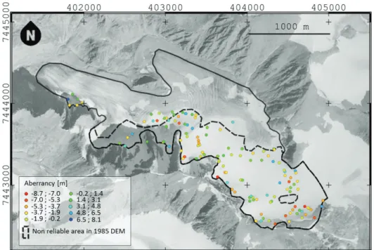
FIGURE 2. 1985 orthophoto. The area south of the dashed line is snow covered and re-sulted in low digital elevation model (DEM) quality. Color-ed dots indicate the points at which 1985 surface elevation was manually measured. The points’ colors indicate their relative deviations from their neighbors within a 100 m di-ameter. Coordinates refer to Universal Transverse Mercator (UTM) zone 22N.
FIGURE 3. Orthophoto from August 2014 obtained by the Structure from Motion (SfM) process, camera positions and ground control points (GCPs). As the 2014 orthophoto is limited to the surroundings of the glacier and its immediate surroundings, it is superimposed on the 1985 orthophoto (monochromatic) to illustrate the estimated extent of the glacier at the end of the Little Ice Age. Coordinates refer to UTM zone 22N.
2015). However, comparison of the 2-m-resolution 2012 SETSM DEM against 1985 and SfM DEM in-dicated that SETSM is subject to a systematic vertical offset in the order of 6 to 10 m (cf. Bjerre and Stentoft, 2015). The difference was measured over stable terrain in vicinity of the glacier and likely related to the 2012 DEM not being tied to ground control points (cf. Noh and Howat, 2015). Furthermore, SETSM shows arti-facts of similar characteristics to those occurring on the 1985 DEM. For these reasons, SfM was deemed better suited for the purpose of calculating geodetic mass balance of Aqqutikitsoq.
The workflow of DEM generation followed the clas-sical SfM process, divided into four steps: (1) pictures acquisition, (2) GPS survey and processing, (3) DEM generation, and (4) accuracy assessment (e.g., Smith et al., 2015; Carrivick et al., 2016).
In the photographic survey we acquired pictures of the glacier, taken from natural viewpoints on the relatively high and steep mountains surrounding the glacier. Four distinct peaks, three of them located on the southwestern side of the glacier and one on the northeastern side, were climbed (Fig. 3). In total, 622 pictures were recorded using two con-sumer-level cameras: Nikon D3100 (10 megapixels) with a Sigma 10-20 mm f/4.5 lens and Nikon D3200 (24.2 megapixels) with a Nikon 18-55 mm f/3.5 lens.
A GPS survey was performed to obtain high-precision coordinates of ground control points (GCPs) to georefer-ence the SfM DEM. In the present study, a Trimble 5700 receiver combined with a Zephyr 4-points feed antenna was used. Because the GCPs need to appear in the SfM pictures, artificial ground targets were installed on the gla-cier during the first day of the survey. However, severe weather made picture acquisition impossible during the
FIGURE 4. 1985 (left) and 2014 (right) DEMs with 25 m contour lines as well as the respective glacier outlines. Magnified sections of the DEMs are shown to highlight the difference in resolution and accuracy between the two models.
following days, and the targets were destroyed by storms and heavy rainfall. Consequently, we decided to use natural GCPs, such as large boulders on the glacier surface, that could not be moved by strong winds. This allowed the survey to be undertaken on separate days, and GPS coor-dinates of the edges of big boulders could be acquired re-gardless of weather conditions, saving the rare days of clear weather for the photogrammetric survey. However, the identification of these natural features in the SfM pictures is not straightforward. To ensure that a minimum number of GCPs will be available, GPS coordinates of natural GCPs were taken intentionally in big quantities (173 points). Out of these, 138 could be non-ambiguously identified in the SfM pictures. GPS coordinates were measured using the post-processing rapid-static approach, which combines high precision and acquisition time of 5–10 s, which al-lowed a fairly quick collection of the large GCP data set. The in situ GPS data were processed using Leica GEO Office (LGO) and base station data from the Sisimiut Ref-erence Station, located at 26 km southwest of the study site. The elevation accuracy of the post-processed GPS coordi-nates estimated by LGO was 0.09 m.
The DEM generation using SfM was divided in five main steps: (1) pictures alignment, point matching, and point cloud generation, (2) densification of the point cloud, (3) mesh generation, (4) georeferencing, and (5) export of the model to a regular grid. The present DEM was generated using the software Agisoft Photoscan, which offers several functions to perform a semi-auto-mated correction for each of the aforementioned steps. Furthermore, the software uses the metadata of each pic-ture to evaluate the lens distortion model, allowing us to treat all the photos together, even if taken by two different cameras and at variable focal lengths and apertures. The criteria used to correct the DEM within the reconstruct-ing process were the removal of clusters or sreconstruct-ingle outliers and the smoothness of the ice surface. Step (3) results in a dimensionless 3D model of the glacier, which was subse-quently georeferenced by manually identifying the GCPs in the pictures that build the model and by assigning
co-ordinates to the identified GCPs. The model was export-ed as a grid of elevation values, that is, a DEM (Fig. 4), and as orthophoto, generated by a mosaic of the pictures used in the reconstruction (Fig. 3). The final SfM DEM was calculated based on a reduced set to 249 pictures (re-moving redundancies and assigning a similar number of pictures to each viewpoint).
Evaluation of DEM Accuracy and
Resolution
The glacier was successfully modeled as a point cloud with 18.2 million points (step [2]) that evenly covered the ice surface and most of the surrounding slopes at a resolution of 1.6 points m–2. The accuracy of the DEM
was assessed by investigating the dependency of mod-el residuals in X, Y, and Z direction on the number of GCPs used for the georeferencing and the spatial distri-bution of GCPs over the DEM area, following an ap-proach similar to Tonkin and Midgley (2016) for UAV surveys. The GCP data set was divided in referencing and validation points. The errors of the two subsets, in the following termed referencing and validation error, were compared performing two tests. Firstly, the DEM was sequentially referenced with a spatially growing cluster of GCPs. Secondly, a cross validation was per-formed by randomly removing 60% of the GCPs and using them as validation points.
The results of the first georeferencing assessment are reported in Table 1 and Figure 5. The results agree with previous findings based on UAV surveys (Tonkin and Midgley, 2016) and show a dependence of the valida-tion error on the spatial extent covered by the GCPs. Validation and referencing errors become comparable in mean and variance when the reference GCPs cover the maximum area coverable by the GCPs, that is, when they are evenly distributed over the entire glacier area.
The cross validation test was performed adhering to the maximum area principle, and the validation GCPs were selected avoiding spatial clusters. The
Kolmogorov-TABLE 1
DEM accuracy assessment: registration and validation errors and related variance for different numbers of ground control points (GCPs).
Number Of GCPs
Area GCP Mean registration error (m) Mean validation error (m) Registration error variance (m) Validation error variance (m) Total DEM area
4 0.0111 –0.17 1.40 0.91 4.62
5 0.0189 –0.20 –2.26 0.82 5.23
6 0.0322 0.26 1.34 0.80 2.37
7 0.1185 0.36 0.79 0.79 1.29
proach described in Korsgaard et al. (2016), which con-sists of using GPS ground control points measured as part of the GPS-based REFGR Greenlandic reference network. Using the software SOCET SET 5.6 from BAE-Systems, multiple DEMs were generated using a suite of different strategies for automated terrain extrac-tion to account for low contrast areas in the photos. Subsequently, the Figure-of-merit values, an indicator of the quality of the terrain extraction, were computed and chosen for each pixel using the NGATE module in SOCET SET 5.6. High values of the Figure-of-merit are interpolations, and low values are elevations meas-ured in several images.
Determining Geodetic Mass Balance
Glacier surface elevation change from 1985 to 2014 was calculated from the 2014 and 1985 DEMs. Because the two DEMs are of differing spatial resolution, the 2014 DEM was down-sampled to the grid size of the 1985 DEM, that is, 10 m. The potential vertical and horizontal shifts between the DEMs were addressed by coregistration, optimizing on the X, Y, and Z Cartesian coordinates to minimize the vertical difference. Coreg-istration was based on areas of stable terrain outside the glacier perimeter where height change is expected to be zero. The coregistration indicates a horizontal mean shift of 1.25 m in the eastern direction, 0.35 m in the northern direction, and 2.3 m in the vertical direction. The standard deviation of the shifts is calculated to be 1.6 m east, 1.0 m north, and 2.0 m vertical. The 1985 DEM was therefore corrected for the mean shifts to avoid systematic errors in calculating the 1985 to 2014 glacier surface elevation change. The standard deviation of the vertical differences of the DEMs in stable areas was used as uncertainty quantification where the area of both DEMs area is considered reliable.
The approach described above allowed calculating glacier surface elevation change for only 50% of the 1985 glacier surface because the 1985 DEM shows pro-nounced triangulation artifacts over most of the upper half of the glacier (Fig. 4). In this area, corresponding to the 1985 accumulation area, automated photogrammetry failed to match pixels on low-contrast snow surfaces (Fig. 2). Visual inspection of the aerial photographs, however, indicated that the snow-covered areas are not completely featureless, and small crevasses, rocks, and irregularities in the snow cover can be recognized. Such features were used to generate manually 192 points of 1985 surface elevation (Fig. 2) in the areas where automated photo-grammetry has failed. Surface elevation at these points is subject to uncertainty because of the manual and some-what subjective process. The uncertainty was quantified
FIGURE 5. Registration and validation errors as functions of the number of the GCPs. Error bars represent residuals’ variance. Note that the glacier surface area covered by the GCPs is proportional to their number. While the registration error does not depend on the number of GCPs, the validation error and its standard deviation decrease with an increasing number of GCPs. At eight GCPs the validation and registration errors become very similar.
Smirnov test on the residuals of four DEMs, each ref-erenced with 20 randomly selected GCPs, highlighted no statistically significant difference among the models. On the basis of this result, we conclude that 20 reference GCPs, evenly distributed over the ice surface, are suf-ficient for georeferencing the DEM. The same test per-formed on the residuals of a DEM georeferenced with the full data set of 138 GCPs confirmed that there is no statistically significant difference to a DEM referenced with 20 randomly but evenly distributed points. Nev-ertheless, the DEM finally used for calculating the geo-detic mass balance (Fig. 4) is the one referenced with the full GCP data set. Analysis of the residuals of the eleva-tions indicates an elevation confidence interval (95%) of 1.87 m for the Z-coordinates. The final DEM was ex-ported on a regular grid at a native resolution of 0.73 m.
1985 Aerial DEM
The aerial photos were recorded in 1985 at a scale of 1:150,000 as part of a Greenland-wide mapping cam-paign taking place during 1978 to 1987. A 25 m DEM and 2 m orthophotograph were produced for the entire ice-free parts of Greenland and the margin of the ice sheet (Korsgaard et al., 2016). Here we used the 1985 images to create an additional DEM in 10 m horizontal resolution (Fig. 4) and a 2 m orthophotograph (Fig. 1). The images were aero-triangulated following the
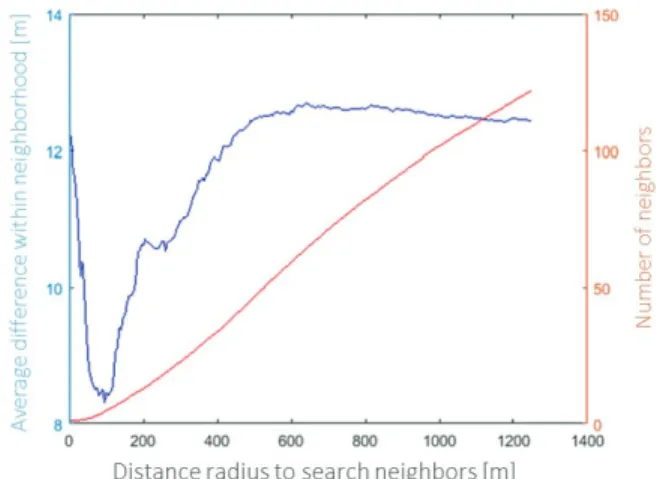
ap-by manually measuring 20 points in the ablation area and comparing their elevation to the respective grid value in the 1985 DEM. This analysis shows a standard devia-tion of 4.3 m between the two methods. However, the identification of points in the snow-covered area is more challenging than in the ablation area. To address this issue, we identified outliers in the manually measured 1985 el-evations by analyzing the surface elevation change (1985 to 2014) at the manually measured points and thereby assumed that neighboring points exhibit similar elevation changes. This assumption is valid within a certain distance radius for which the lowering of the glacier’s surface can be considered homogeneous. This distance was evaluated by finding the points’ average deviation within a varying size neighborhood (from 50 to 1200 m). Average devia-tion is minimal (8.4 m) within a neighborhood of 100 m (Fig. 6). The value of minimal average deviation was defined as the maximal accepted variation of the surface lowering within a 100 m radius. Subsequently, elevation change at each point was compared to its neighboring points within a 100 m buffer. Points deviating more than the maximal accepted variation of the surface lowering were considered outliers and discarded. After the filtering, 112 points were left. The manually generated and filtered points were subsequently used to calculate 1985 to 2014 elevation change for the 1985 accumulation area.
We calculated spatially continuous surface elevation change over the 1985 accumulation area using a kriging approach (e.g., Rippin et al., 2011; Carrivick et al., 2015). Because the manually extracted elevations are rather sparse in the area, surface elevation change obtained from DEM differencing over the 1985 ablation area was used
to calibrate the method. Firstly, a linear trend between el-evation and ice thickness change was observed, indicating glacier loss is smaller at higher altitudes. Hence, we ap-plied universal kriging, using elevation as a regression var-iable (Isaaks and Srivastava, 1989). Secondly, the empirical semivariogram was computed on elevation changes in the 1985 accumulation area (i.e., at the points for which the 1985 surface elevation was determined manually) and 112 randomly selected samples of ice thickness changes in the 1985 ablation area (i.e., determined from direct DEM differencing). This way, we modeled the semivari-ance using both data from the ablation and accumulation area, ensuring the consistency of the spatial variability of the ice thickness change process over the entire glacier. The empirical semivariogram was fitted using a spherical model. The semivariogram was evaluated and modeled using the R functions “variogram” and “vgm,” whereas the universal kriging interpolation was performed using the function “krige”; both are available in the package “gstat” (Pebesma, 2004). Eventually, we joined the grid-ded surface elevation change resulting from kriging in-terpolation (1985 accumulation area) with the grid of elevation changes derived from DEM subtraction (1985 ablation area) into a grid of elevation changes covering the entire 1985 glacier area (Fig. 7).
Ice Thickness Distribution and Ice
Volume
A total of 37 GPR profiles were collected in the field from which we retrieved the ice thickness and estimated the total ice volume of Aqqutikitsoq glacier. An ideal grid where the survey lines extend over the entire glacier was envisaged, but had to be adapted (Fig. 8) because of inac-cessible areas that include crevasses and areas with a risk of rock fall. The glacier was mostly depleted of firn and snow and, consequently, all measurements were carried out on an ice surface. The GPR unit used was a Malå ProEx combined with a 50 MHz Rough Terrain An-tenna. The ice thickness profiles were obtained by con-tinuously moving the GPR on the glacier surface along survey lines, thereby keeping the transmitter and receiver, included in the flexible hose-shaped antenna, at a fixed geometry. The spatial position of the GPR was continu-ously recorded from a hand-held GPS. The accuracy of the GPS receiver in the X and Y direction was a few meters. For the conversion of travel time of the GPR signal to ice thickness, a mean velocity of 0.168 m ns–1
of electromagnetic waves in glacier ice was applied. The value was considered appropriate for a polythermal gla-cier based on Bogorodsky et al. (1985), Bælum and Benn (2011), Pettersson and Holmlund (2003), Cuffey and Pat-erson (2010), Friedt et al. (2013), and Ai et al. (2014).
FIGURE 6. Average deviation of surface lowering (1985 to 2014) at the manually selected points, expressed as a function of horizontal distance. For a neighborhood distance of 100 m, the deviation is minimal, that is, 8.4 m. On average, we find 4.5 neighboring points within 100 m.
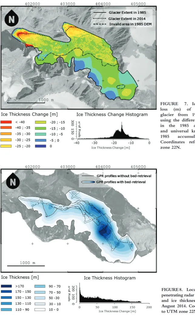
FIGURE 7. Ice thickness loss (m) of Aqqutikitsoq glacier from 1985 to 2014 using the difference of DEMs in the 1985 ablation area and universal kriging in the 1985 accumulation area. Coordinates refer to UTM zone 22N.
FIGURE 8. Location of ground penetrating radar (GPR) profiles and ice thickness distribution, August 2014. Coordinates refer to UTM zone 22N.
The software ReflexW (version 7.1.4) was used for post-processing the GPR profiles and identify-ing the bedrock. Four filters were applied: (1) subtract mean (dewow) filter for removing low frequency parts, (2) manual gain filter to enhance signals from greater depths, (3) 2D background removal filter for removing temporally consistent noise, and (4) 1D bandpass But-terworth filter to eliminate very low and high frequency parts. Tentatively, we migrated selected radar transects. Interpretation of bed topography from the bed returns, however, did not change in our case and consequently we decided to skip migration of the remaining data.
The analysis of the radar data shows for many profiles the characteristics of a polythermal glacier with cold ice nearly transparent on top and strong internal reflections from temperate ice closer to the bed (cf. Bamber, 1988; Pettersson and Holmlund, 2003). Attention was paid not to misinterpret the interface of cold and temperate ice for the glacier bed. Where an unambiguous bed-return was missing, no glacier bed was mapped. The error of the in-terpretation of GPR profiles was evaluated through quan-tification of the residuals in ice thickness at all intersecting profiles, that is, by crossover analysis. The total number of intersections is 16, and the standard deviation of the dif-ferences is 1.9 m. A continuous bedrock topography was then obtained by ordinary kriging using the ice thickness measurements and the glacier outline (ice thickness equals zero) obtained from the 2014 SfM orthophoto (Binder et al., 2009; Rippin et al., 2011; Williams et al., 2016).
r
eSultSIce Thickness Distribution and Ice
Volume
A total of 18.5 km of GPR profiles was measured. Thereof, 8.5 km are interpreted as showing
unambigu-ous bed returns (Fig. 8). The remaining profiles of lack-ing or ambiguous bed return were discarded. Most of the profiles show cold ice at the top and temperate ice close to the glacier bed. The cold ice layer is typically a few decameters thick; however, at certain locations the radar data are nearly free of internal scatter down to the bedrock at 140 m depth and thus indicate that locally the ice column might be entirely cold.
On the basis of interpolated ice thickness, the total ice volume of Aqqutikitsoq glacier is estimated to be 148.6 ± 47.7 106 m3 in August 2014 (Table 2). The
uncertainty of the ice volume was first quantified at each grid cell using the spatially distributed semivari-ance associated with the ordinary kriging interpola-tion. Then, total volume uncertainty was calculated by summing the root square of the semivariance (i.e., the standard deviation) of each grid cell over the entire glacier area.
The maximum depth in Aqqutikitsoq glacier is meas-ured to be 174 m (cf. Fig. 8). The average ice thickness over the entire glacier is calculated to be 51.8 ± 16.6 m. The mean measured ice thickness calculated solely from the GPR profiles is 63.8 m. The difference from the cal-culated ice thickness is explained by the fact that steep and shallow areas could not be measured.
Geodetic Volume and Mass Balance
The surface elevation change over the 1985 glacier area is between –10 and –30 m in most areas, and the average elevation change equals –17.4 ± 3.3 m. On the two tongues, however, the surface lowering reaches val-ues from 40 to almost 60 m (Fig. 7). Areas with limited elevation change are primarily located at higher alti-tudes and on the north-facing mountainside. Uncer-tainties in calculated elevation changes are because of the digitizing error in the 1985 accumulation area and
TABLE 2
Volumes and uncertainty calculation for ice thickness in 2014 and volume change between 1985 and 2014.
Glacier volume Δh
Surface 2014 Ablation area Accumulation area Entire glacier Computation method GPR + ordinary
kriging
Difference of DEMs 1985 and 2014
Manual points selection and universal kriging
Sum of the two surfaces
Uncertainty estimation method
Square root
semivariance map σ of difference in altitudes in stable areas σ between manual points and 1985 in ablation area
Each surface has its uncertainty
Uncertainty (5.3–29.9) m 2.0 m 4.3 m 2.0 m; 4.3 m Volume estimation (106 m3) 148.623 30.156 19.653 49.809
Total Uncertainty (106 m3) 47.645 3.111 6.285 9.396
the coregistration error between the two DEMs in the 1985 ablation area (cf. Table 2)
Over the 1985 ablation area, the total volume change is 30.2 ± 3.1 106 m3. For the 1985 accumulation area,
the universal kriging extrapolation calculates a volume change of 19.7 ± 6.3 106 m3. Volume change is
con-verted to mass change assuming an average density of 850 ± 60 kg m–3 (cf. Huss, 2013), yielding a mass loss of
0.042 ± 0.008 Gt.
Given the unique data set that combines volume measurements with geodetic mass balance, the relative volume loss of the Aqqutikitsoq glacier is estimated to be between 23.2% and 28.6% of its 1985 volume. This estimation is based on the extremes in the uncertainties of the ice thickness and thickness change, as presented in Table 3. This results in a range of possible values of relative volume change, which is here expressed as the mean range value ± the range’s amplitude, that is, 25.9% ± 2.7%.
d
IScuSSIonQuality of the SfM Elevation Model and
Geodetic Mass Balance
The 2014 DEM is affected by three sources of uncer-tainty: the position accuracy of the GCPs, the georefer-encing process, and the systematic deformations induced by the software in the model. The elevation confidence interval of the 2014 DEM (1.87 m) is about one order of magnitude greater than the GCPs coordinates’ preci-sion (0.09 m), indicating that GPS accuracy does not contribute substantially to the overall error.
Deformations of the model introduced by the soft-ware have not been directly assessed. However, the survey strategy based on collecting pictures on a
near-circular orbit around the glacier, varying the distance and the inclination of the camera with respect to the target, is expected to produce DEM errors in the order of magnitude of 0.1 m (James and Robson, 2014).
The georeferencing process is the main error source of the 2014 DEM. Georeferencing requires localizing the GCPs in the pictures where the pixels have a ground resolution ranging from tens of centimeters to meters, depending on the distance between the GCP and the camera. Hence, the identification of the GCPs in the pictures is sometimes ambiguous and subject to user in-terpretation.
The georeferencing error is absolute with respect to an absolute reference system. However, the geodetic mass balance is calculated from the coregistered 2014 and 1985 DEMs, rendering this source of error irrel-evant in the context of a relative registration. Therefore, considering the major sources of uncertainty, that is, limitations in the 1985 DEM, we conclude that the SfM DEM does not contribute significantly to the overall uncertainty of calculated geodetic mass balance.
In the 1985 accumulation area, the uncertainty sources had to be addressed differently from the ablation area, as they are associated to the process of manual el-evation measurements for selected points. The semivari-ance map produced by the universal kriging interpola-tion, however, results in values that are smaller than 4.3 m, which is the value obtained by comparison of surface elevation at manually measured points and automatically derived 1985 DEM. Therefore, 4.3 m of uncertainty was used as a more conservative estimate. Even this estimate, however, might be optimistic. The value of 4.3 m was derived over the 1985 ablation area where the glacier surface is of high contrast and manually measuring sur-face elevation at selected point locations was arguably easier than in the 1985 accumulation area.
TABLE 3
Length, area, volume, and ice thickness of Aqqutikitsoq glacier in 1985 and 2014, as well as absolute and relative changes in the aforementioned parameters.
1985 2014 Absolute change Relative change (%) Length (km) 4.22 4.05 –0.17 –4 Planar area (106 m2) 3.05 2.87 –0.18 –5.8 Ice volume (106 m3) 255.5(1) 196.3(1) –59.2(1) –23.2(1) 141.3(2) 101.0(2) –40.4(2) –28.6(2) Mean thickness (m) 83.8(1) 68.4(1) –15.4(1) –18.4(1) 46.4(2) 35.2(2) –11.2(2) –24.1(2)
(1)Values calculated with maximum expected ice thickness in 2014 and maximal volume change between 1985 and 2014. (2)Values calculated with minimum expected ice thickness in 2014 and minimum volume change between 1985 and 2014.
Measured Ice Thickness and Calculated
Ice Volume
The main source of error in the ice thickness meas-urement is considered to be the interpretation and digi-tization of the GPR profiles. Uncertainty in interpreta-tion of the GPR profiles is 1.9 m, as indicated by the crossover analysis. Given the available GPR equipment, it was not possible to validate the propagation veloc-ity of 0.168 m s–1 through a common midpoint survey.
Instead, we relied on propagation velocities measured in polythermal glaciers in earlier studies. Published values do not vary strongly, and uncertainty related to our ve-locity assumptions is thus assumed to be relatively small. The interpolated ice thickness appears realistic and shows a typical distribution with thick glacier ice under-neath the flat glacier sections and thinner ice in steeper sections (e.g., Haeberli and Hölzle, 1995). The distribu-tion of radar profiles in the flat upper secdistribu-tion of the glacier is relatively dense and allows for a reliable interpolation and assessment of ice volume where the glacier is thickest and most of its ice is stored. Nevertheless, ice thickness interpolation is the major source of uncertainty in
esti-mating Aqqutikitsoq glacier volume and can locally reach 30 m (Fig. 9 and Table 2). Uncertainty resulting from in-terpretation of the GPR profiles (1.9 m) is relatively small compared to the nugget of the kriging semivariogram (5.3 m, cf. Fig. 9). This is because a considerable fraction of the glacier area lacks GPR data (cf. Figs. 8 and 9). These areas at the orographically left glacier perimeter were in-accessible mainly due to crevasses and risk of rock fall from the steep adjacent slopes. The ice thickness for these areas has thus been derived from interpolation between the GPR measurements and the ice margin where ice thickness is 0 m. The influence of these glacier sections on overall uncertainty in ice volume estimation is some-what reduced by the general steepness and thus relatively small ice thickness.
Volume Loss in a Local to Global
Context
From 1985 to 2014, Aqqutikitsoq glacier has lost sub-stantial amounts of ice at all elevations. Ice loss is maxi-mal at the tongue, where thinning rates exceed 1 m a–1.
However, even at high elevations, average thinning rates
FIGURE 9. Uncertainty in the bedrock reconstruction given by the ordinary kriging approach (plot 1 in upper left). Three transects are shown (plots 2, 3, and 4) and vertically exaggerated by a factor 3 to visualize the surface lowering of the glacier surface and the uncertainty in bedrock interpolation.
amount to >0.3 m a–1. It appears the glacier has no
ac-cumulation area left nowadays, which is underlined by our 2014 orthophoto (Fig. 3) showing only marginal patches of remaining snow. The glacier is thus very likely to disappear, even if climate does not change any further. Bolch et al. (2013) and Gardner et al. (2013) used ICESat data to assess volume change of glaciers and ice caps for all of Greenland. However, ICESat data cover only a relatively short time period (2003 to 2009), and the measurements along widely spaced lines require ex-tensive extrapolation involving a considerable level of uncertainty. After Mittivakkat glacier on the southeast coast (cf. Yde et al., 2014), Aqqutikitsoq is only the sec-ond glacier on Greenland with detailed and longer-term volume change data. While Aqqutikitsoq glacier volume decreased from ~0.2 km3 to ~0.14 km3 (~25%) over the
time period 1985 to 2014, the larger Mittivakkat glacier (15.8 km2 in 2012) decreased from 2.02 km3 to 1.44
km3 ( ~29%) in the period 1994–2012 (Yde et al., 2014).
Because Mittivakkat did not change substantially from 1981 to 1994 (Knudsen and Hasholt, 1999) relative vol-ume losses of both glaciers are rather similar at roughly a quarter of their early or mid-1980s volumes. Obviously, at a given rate of thinning a thinner glacier will experi-ence a larger relative volume loss.
The measured 1985–2014 thinning rate of ~0.6 m a–1 at Aqqutikitsoq glacier is similar to, for example, the
observed mean geodetic mass balance for 1980–2010 for all glaciers of the Swiss Alps (–0.62 ± 0.07 m w.e. a–1; Fischer et al., 2015). While the sample of measured
Greenland glaciers is much smaller and also observation periods differ slightly, our data from Aqqutikitsoq and the studies on Mittivakkat (Yde et al., 2014) indicate that current changes on Greenland are similar to mid-latitude glaciers. The data set for Aqqutikitsoq glacier thus makes a small but valuable contribution to an im-proved understanding of Greenland glacier changes and will, we hope, motivate further research on the chang-ing ice masses surroundchang-ing the Greenland ice sheet.
c
oncluSIonOur study demonstrates the usefulness of ground-based SfM in establishing high-quality DEMs over a smaller (2.85 km2) valley glacier. The advantages of
the method are low cost, low resources (e.g., no UAV needed), and flexibility as the required images and GCPs can be acquired with limited logistical effort. Using these advantages and combining the SfM survey with GPR measurements, a comprehensive data set describ-ing surface topography and ice thickness of a glacier was compiled. The data are of particular interest as our measurements constitute the first such detailed data set
for a glacier on Greenland’s west coast. Therefore, the Aqqutikitsoq ice thickness measurements have already been extensively used as one of 18 globally distributed test glaciers in the “ice thickness models intercompari-son experiment” (ITMIX) (Farinotti et al., 2017).
We have explored the applicability of a newly avail-able Greenland-wide DEM for the 1970s to 1980s (here in this study 1985) to assess geodetic mass balance of a glacier. In the case of Aqqutikitsoq glacier, extended low-contrast areas in the aerial photos from 1985 cause a number of challenges that have been addressed by manual determination of 1985 surface height at point locations in low surface contrast areas. While this allowed calculation of geodetic mass balance of Aqqutikitsoq over the time period 1985 to 2014, the manual approach appears chal-lenging for application to larger glacier samples.
Our findings indicate substantial mass loss of the in-vestigated glacier, which lost 25.9% ± 2.7% of its vol-ume over the past three decades. With the historical DEM at hand and new DEMs becoming available (e.g., TanDEM-X, ArcticDEM; Zink et al., 2014; Noh and Howat, 2015), we suggest that the investigations could be extended to larger glacier samples to assess Aqqu-tikitsoq’s representativeness in a wider context.
a
cknowledgMentSWe thank the editors and the two anonymous re-viewers for their thorough and very valuable comments. This study is based on the field measurements and anal-ysis carried out as student projects in the course “11427 Arctic Technology” at DTU ARTEK. We greatly ac-knowledge the entire “2nd Fjord” field team and Carl E. Bøggild for assistance in the field and in field-work or-ganization. We thank Gunvor M. Kirkelund for organ-izing and leading course 11427 as well as the secretaries and the technicians for their most valuable assistance, which made Aqqutikitsoq field measurements possible. The community of Qeqqata is acknowledged for host-ing course 11427. H. Machguth is partly financed under the project Glaciers_cci (4000109873/14/I-NB). A. A. Bjørk is funded by the “X_Centuries Project”, Danish Council for Independent Research (FNU) (grant no. 0602-02526B). This publication is contribution number 73 of the Nordic Centre of Excellence SVALI, “Stability and Variations of Arctic Land Ice” funded by the Nordic Top-level Research Initiative (TRI).
r
eferenceSc
ItedAhlstrøm, A. P., Bøggild, C. E., Olesen, O. B., Petersen, D., and Mohr, J. J., 2007: Mass balance of the Amitsulôq ice
cap, West Greenland glacier mass balance changes and meltwater discharge. In Ginot, P., and Sicart, J.-E. (eds.), Selected Papers from Sessions at the IAHS Assembly in Foz do Iguaçu, Brazil, 2005. IAHS Publication 318: 107– 115.
Ai, S., Wang, Z., E, D., Holmén, K., Tan, Z., Zhou, C., and Sun, W., 2014: Topography, ice thickness and ice volume of the glacier Pedersenbreen in Svalbard, using GPR and GPS.
Polar Research, 33: 18533, doi: http://dx.doi.org/10.3402/
polar.v.33.18533.
Bælum, K., and Benn, D. I., 2011: Thermal structure and drainage system of a small valley glacier (Tellbreen, Svalbard), investigated by ground penetrating radar. Cryosphere, 5: 139–149.
Bamber, J. L., 1988: Enhanced radar scattering from water inclusions in ice. Journal of Glaciology, 34(118): 293–296. Binder, D., Bruckl, E., Roch, K. H., Beh,, M., Schoner, W.,
and Hynek, D., 2009: Determination of total ice volume and ice-thickness distribution of two glaciers in the Hohe Tauren region, Eastern Alps, from FPR data. Annals of
Glaciology, 50(51): 71–79.
Bjerre, E., and Stentoft, P., 2015: Estimating Volume and Volume
Change of a Small Greenlandic Glacier with Geophysical Methods.
B.Sc. thesis, DTU Technical University of Denmark, Kgs. Lyngby, 90 pp.
Bjørk, A. A., Kruse, L. M., and Michaelsen, P. B., 2015: Brief Communication: Getting Greenland’s glaciers right—A new dataset of all official Greenlandic glacier names.
Cryosphere, 9: 2215–2218, doi: http://dx.doi.org/10.5194/
tc-9-2215-2015.
Boas, L., and Wang, P. R., 2011: Weather and Climate Data from
Greenland 1958–2010, Observation Data with Description.
Copenhagen: Danish Meteorological Institute, DMI Technical Report 11-15.
Bøggild, C. E., 2000: Preferential flow and melt water retention in cold snow packs in West-Greenland. Nordic
Hydrology, 31: 287–300.
Bogorodsky, V., Bentley, G., and Gudmandsen, P., 1985:
Radioglaciology, Dordrecht: D. Reidel.
Bolch, T., Sørensen, L. S., Simonsen, S., Mölg, N., Machguth, H., Rastner, P., and Paul, F., 2013: Mass change of local glaciers and ice caps on Greenland derived from ICESat data. Geophysical Research Letters, 40: 875–881.
Braithwaite, R., and Raper, S., 2009: Estimating equilibrium-line altitude (ELA) from glacier inventory data. Annals of
Glaciology, 50: 127–132.
Carrivick, J. L., Berry, K., Geilhausen, M., James, M., Williams, M. H. M., Brown, L.E., Rippin, D. M., and Carver, S. J., 2015: Decadal-scale changes of the Odenwinkelkees, central Austria, suggest increasing control of topography and evolution towards steady state. Geografiska Annaler:
Series A, Physical Geography, 97: 543–562, doi: http://dx.doi.
org/10.1111/geoa.12100.
Carrivick, J. L., Smith, M. W., and Quincey, D. J., 2016: Structure
from Motion in the Geosciences. Oxford: Wiley-Blackwell, 208 pp.
Cuffey, K. M., and Paterson, W. S. B., 2010: The Physics
of Glaciers, fourth edition. Burlington, Massachusetts:
Butterworth-Heinemann/Elsevier.
Farinotti, D., Brinkerhoff, D., Clarke, G. K., Fürst, J. J., Frey, H., Gantayat, P., Gillet-Chaulet, F., Girard, C., Huss, M., Leclercq, P. W., Linsbauer, A., Machguth, H., Martin, C., Maussion, F., Morlighem, M., Mosbeux, C., Pandit, A., Portmann, A., Rabatel, A., Ramsankaran, R., Reerink, T. J., Sanchez, O., Stentoft, P. A., Kumari, S. S., van Pelt, W. J., Anderson, B., Benham, T., Binder, D., Dowdeswell, J. A., Fischer, A., Helfricht, K., Kutuzov, S., Lavrentiev, I., McNabb, R., Gudmundsson, G. H., Li, H., and Andreassen, L. M., 2017: How accurate are estimates of glacier ice thickness? Results from ITMIX, the Ice Thickness Models Intercomparison eXperiment. The
Cryosphere, 11(2): doi:
http://dx.doi.org/10.5194/tc-11-949-2017.
Fischer, M., Huss, M., and Hoelzle, M., 2015: Surface elevation and mass changes of all Swiss glaciers 1980–2010.
The Cryosphere, 9: 525–540.
Fonstad, M. A., Dietrich, J. T., Courville, B. C., Jensen, J. L., and Carbonneau, P. E., 2013: Topographic structure from motion: a new development in photogrammetric measurements. Earth, Surface Processes and Landforms, 38: 421–430.
Friedt, J.-M., Saintenoy, A., Marlin, C., Booth, A., Laffly, D., Tolle, F., Bernard, E., and Griselin, M., 2013: Deriving ice thickness, glacier volume and bedrock morphology of Austre Lovenbreen (Svalbard) using GPR. Near Surface
Geophysics, 11(2): 253–261.
Gardner, A. S., Moholdt, G., Cogley, J. G., Wouters, B., Arendt, A. A., Wahr, J., Berthier, E., Hock, R., Pfeffer, W. T., Kaser, G., Ligtenberg, S. R. M., Bolch, T., Sharp, M. J., Hagen, J. O., van den Broeke, M. R., and Paul, F., 2013: A reconciled estimate of glacier contributions to sea level rise: 2003 to 2009. Science, 340: 852–857.
Gärtner-Roer, I., Naegeli, K., Huss, M., Knecht, T., Machguth, H., and Zemp, M., 2014: A database of worldwide glacier thickness observations. Global and Planetary Change, 122: 330–344.
Haeberli, W., and Hölzle, M., 1995: Application of inventory data for estimating characteristics of and regional climate-change effects on mountain glaciers: a pilot study with the European Alps. Annals of Glaciology, 21: 206–212.
Huss, M., 2013: Density assumptions for converting geodetic glacier volume change to mass change. Cryosphere, 7: 877– 887.
Isaaks, E. H., and Srivastava, R. M., 1989: Applied Geostatistics. New York: Oxford University Press.
James, M. S., and Robson, S., 2014: Mitigating systematic error in topographic models derived from UAV and ground-based image networks. Earth Surface Processes
and Landforms, 39: 1413–1420, doi: http://dx.doi.
org/10.1002/esp.3609.
Kjær, K. H., Khan, S. A., Korsgaard, N. J., Wahr, J., Bamber, J. L., Hurkmans, R., van den Broeke, M., Timm, L. H., Kjeldsen, K. K., Bjørk, A. A., Larsen, N. K., Jørgensen, L. T., Færch-Jensen, A., and Willerslev, E., 2012: Aerial photographs reveal late-20th-century dynamic ice loss in northwestern Greenland. Science, 337: 569–573.
Knudsen, N. T., and Hasholt, B., 1999: Radio-echo sounding at the Mittivakkat Gletscher, Southeast Greenland. Arctic,
Antarctic, and Alpine Research, 31: 321–328.
Korsgaard, N. J., Nuth, C., Khan, S. A., Kjeldsen, K. K., Bjørk, A. A., Schomacker, A., and Kjær, K. H., 2016: Digital elevation model and orthophotographs of Greenland based on aerial photographs from 1978–1987. Scientific Data, 3: 160032, doi: http://dx.doi.org/10.1038/sdata.2016.32. Krabill, W., Abdalati, W., Frederick, E., Manizade, S., Martin,
C., Sonntag, J., Swift, R., Thomas, R., Wright, W. and Yungel, J., 2000: Greenland Ice Sheet: high-elevation balance and peripheral thinning. Science, 289: 428–430.
Machguth, H., Thomsen, H., Weidick, A., Ahlstrøm, A. P., Abermann, J., Andersen, M. L., Andersen, S., Bjørk, A. A., Box, J. E., Braithwaite, R. J., Bøggild, C. E., Citterio, M., Clement, P., Colgan, W., Fausto, R. S., Gleie, K., Gubler, S., Hasholt, B., Hynek, B., Knudsen, N., Larsen, S., Mernild, S., Oerlemans, J., Oerter, H., Olesen, O., Smeets, C., Steffen, K., Stober, M., Sugiyama, S., van As, D., van den Broeke, M. and van de Wal, R. S. (2016): Greenland surface mass-balance observations from the ice-sheet ablation area and local glaciers. Journal of Glaciology, 62(235): doi: http:// dx.doi.org/10.1017/jog.2016.75.
Nielsen, J. D., 1999: The Determination of the Water Resources
in the Pisigsarfik Catchment Area in Greenland Using an Energy Balance Approach and GIS. Master thesis, Geological
Institute, University of Aarhus, Denmark.
Noh, M., and Howat, I., 2015: Automatic stereo photogrammetric DEM generation at high latitudes: Surface Extraction from TIN-based Search-space Minimization (SETSM) validation and demonstration over glaciated regions. GIScience and Remote Sensing, 52: 198-217.
Olesen, O. B., 1986: Fourth year of glaciological field work at Tasersiaq and Qapiarfiup sermia, West Greenland. Rapport
Grønlands Geologiske Undersøgelse, 130: 121–126.
Pebesma, E. J., 2004: Multivariable geostatistics in S: the gstat package. Computers & Geosciences, 30(7): 683–691.
Pettersson, R., Jansson, P., and Holmlund, P., 2003: Cold surface layer thinning on Storglaciären, Sweden, observed by repeated ground penetrating radar surveys. Journal of
Geophysical Research, 108(F1): 2156–2202.
Piermattei, L., Carturan, L., and Guarnieri, A., 2015: Use of terrestrial photogrammetry based on structure from motion for mass balance estimation of a small glacier in the Italian Alps. Earth Surface Processes and Landforms, 40: 1791–1802. Rastner, P., Bolch, T., Mölg, N., Machguth, H., Le Bris, R.,
and Paul, F., 2012: The first complete inventory of the local glaciers and ice caps on Greenland. Cryosphere, 6: 1483– 1495.
Rippin, D. M., Carrivick, J. L., and Williams, C., 2011: Evidence towards a thermal lag in the response of Kårsaglaciären,
northern Sweden, to climate change. Journal of Glaciology, 57: 895–903.
Ryan, J. C., Hubbard, A. L., Box, J. E., Todd, J., Christoffersen, P., Carr, J. R., Holt, T. O., and Snooke, N., 2015: UAV photogrammetry and structure from motion to assess calving dynamics at Store Glacier, a large outlet draining the Greenland Ice Sheet. The Cryosphere, 9: 1–11.
Smith, M. W., Carrivick, J. L., and Quincey, D. J., 2016: Structure from motion photogrammetry in physical geography. Progress in Physical Geography, 40(2): 247–275. Sørensen, L. S., Simonsen, S. B., Nielsen, K., Lucas-Picher, P.,
Spada, G., Adalgeirsdottir, G., Forsberg, R., and Hvidberg, C. S., 2011: Mass balance of the Greenland ice sheet (2003– 2008) from ICESat data—The impact of interpolation, sampling and firn density. The Cryosphere, 5: 173–186. Thomson, L., and Copland, L., 2016: White Glacier 2014,
Axel Heiberg Island, Nunavut: mapped using Structure from Motion methods. Journal of Maps, 12(5): 1063–1071. Tonkin, T. N., and Midgley, N. G., 2016: Ground-control
networks for image based surface reconstruction: an investigation of optimum survey designs using UAV derived imagery and Structure-from-Motion photogrammetry.
Remote Sensing, 8: 786, doi: http://dx.doi.org/10.3390/
rs8090786.
Van de Wal, R. S. W., Boot, W., Smeets, C. J. P. P., Snellen, H., van den Broeke, M. R., and Oerlemans, J., 2012: Twenty-one years of mass balance observations along the K-transect, West Greenland. Earth Systems Science Data, 4: 31–35. Weidick, A., 1959: Glacier variations in West Greenland in
historical time. Meddelelser om Grønland, 158(4).
Westoby, M. J., Brasington, J., Glasser, N. F., Hambrey, M. J., and Reynolds, J. M., 2012: ‘Structure-from-Motion’ photogrammetry: a low-cost, effective tool for geoscience applications. Geomorphology, 179: 300–314.
Williams, C. N., Carrivick, J. L., Evans, A. J., and Rippin, D. M., 2016: Quantifying uncertainty in using multiple datasets to determine spatiotemporal ice mass loss over 101 years at Karsaglaciaren, arctic Sweden. Geografiska Annaler,
Series A: Physical Geography, 98: 61–79, doi: http://dx.doi.
org/10.1111/geoa.12123.
Yde, J. C., Gillespie, K., Løland, R., Ruud, H., Mernild, S. H., De Villiers, S., Knudsen, N. T., and Malmros, J. K., 2014: Volume measurements of Mittivakkat Gletscher, southeast Greenland. Journal of Glaciology, 60: 1199–1207.
Zink, M., Bachmann, M., Bräutigam, B., Fritz, T., Hajnsek, I., Krieger, G., Moreira, A., and Wessel, B., 2014: TanDEM-X: the new global DEM takes shape. IEEE Geoscience and
Remote Sensing Magazine, 2: 8-23.
MS submitted 10 August 2016 MS accepted 22 May 2017