Digital pre-compensation for faulty D/A converters : the "missing pixel" problem

Digital Pre-Compensation for Faulty D/A Converters:

The "Missing Pixel" Problem

by

Sourav Raj Dey

Submitted to the Department of Electrical Engineering and Computer Science

in partial fulfillment of the requirements for the degree of

Master of Engineering in Electrical Engineering and Computer Science

at the

MASSACHUSETTS INSTITUTE OF TECHNOLOGY

June 2004

@Massachusetts

Institute of Technology, 2003. All rights reserved.

The author hereby grants to M.I.T. permission to reproduce and distribute publicly

paper and electronic copies of this thesis and to grant others the right to do so.

AA

Author ...

...

.

.

.

.

.

Department of Elec rical Engineering and Computer Science

December 14, 2003

I1I

Certified by...

..

.

...

Alan V. Oppenheim

Ford Professor of Engineering

Thesis Supervisor

Accepted by. ... . . . . .. .. .. .

Arthur C. Smith

Chairman, Department Committee on Graduate Students

MASSACHUSETTS INSTMJ)TE

OF TECHNOLOGY

JUL 2 0 2004

Digital Pre-Compensation for Faulty D/A Converters:

The "Missing Pixel" Problem

by

Sourav Raj Dey

Submitted to the Department of Electrical Engineering and Computer Science on December 14, 2003, in partial fulfillment of the

requirements for the degree of

Master of Engineering in Electrical Engineering and Computer Science

Abstract

In some contexts, DACs fail in such a way that specific samples are dropped. The dropped samples lead to distortion in the analog reconstruction. We refer to this as the "missing pixel" problem. Under certain conditions, it may be possible to compensate for the dropped sample by pre-processing the digital signal, thereby reducing the analog reconstruction error. We develop three such compensation strategies in this thesis.

The first strategy uses constrained minimization to calculate the optimal finite-length compensation signal. We develop a closed-form solution using the method of Lagrange multipliers. Next, we develop an approximation to the optimal solution using discrete prolate spheroidal sequences. We show that the optimal solution is a linear combination of the discrete prolates. The last compensation technique we develop is an iterative solution in class of projection-onto-convex-sets. We develop the algorithm and prove that it converges to the optimal solution found using constrained minimization. Each of the three strategies are analyzed and results from numerical simulations are presented.

Thesis Supervisor: Alan V. Oppenheim Title: Ford Professor of Engineering

Acknowledgments

Foremost, I would like to thank my adviser, Al Oppenheim, for his mentorship and guidance. For taking me under his wing as a "green" undergraduate and shaping me into a better engineer, researcher, and person. I hope this is just the beginning of a lifelong collaboration through my doctoral studies and beyond.

I want to also thank the other professors and teachers that have helped me along the way, at MIT, Seoul International School, and Elizabethtown. Your support has brought me here.

To the DSPG members, thanks for making this place the intellectual playground that it is. My conversations with you guys, Andrew, Vijay, Petros, Charles, and Maya have gone a long way to making this thesis a reality. Thanks must also go out to my friend, Ankit, for the many long nights brainstorming on a cheap Home Depot white-board mounted on the wall of our apartment. To all my other friends, especially Sachin, Pallabi, and Arny, thank you for supporting me, both mentally and emotionally, in a very hectic year.

Lastly, to my family. You have been the greatest support of all. Wherever in the world we may live, home is always where my heart is. Piya, you're the greatest sister in the world. Thotho. To my parents, this thesis is culmination of a lifetime of love and support. Thank you for always guiding and pushing me to be all that I can be.

Contents

1 Introduction ₁₃ 1.1 Problem Statement . . . . 14 1.2 Constraints . . . . 18 1.2.1 _{Oversampling . . . . 18} 1.2.2 Symmetric Compensation . . . . 20 1.3 _{Previous Work . . . . 21} 1.3.1 Alternative Formulation . . . . 21 1.3.2 Perfect Compensation . . . . 22

1.3.3 Missing Pixel Compensation . . . . 23

1.4 Thesis Outline . . . . 23 2 Constrained Minimization ₂₅ 2.1 _{Derivation . . . . 25} 2.2 Performance Analysis . . . . 28 2.2.1 Examples . . . . 28 2.2.2 _{Error Performance . . . . 30} 2.2.3 _{Computational Complexity . . . . 30} 2.3 _{Numerical Stability . . . . 31}

3 Discrete Prolate Approximation ₃₃ 3.1 _{Derivation . . . . 33}

3.1.1 _{W indowing and Discrete Prolate Spheroidal Sequences . . . . 33}

3.1.2 _{Extremal Properties of the DPSS . . . . 35}

3.1.3 _{Duality of DPSS . . . . 36}

3.2.1 3.2.2

Different Constraints . . . . Constrained Mimimization Solution in th 3.3 Performance Analysis . . . . 3.3.1 Examples . . . . 3.3.2 Error performance . . . . 3.3.3 Computational Complexity . 3.4 Numerical Stability . . . . 4 Iterative Minimization 4.1 D erivation . . . . 4.1.1 Convergence . . . . 4.1.2 Uniqueness . . . . 4.1.3 Existence . . . . 4.2 Performance Analysis . . . . 4.2.1 Exam ples . . . . 4.2.2 Convergence Rate . . . . A DPSS and the Singular Value Decomposition

A.1 Singular Value Decomposition . . . . A.2 Discrete Prolate Spheroidal Sequences . . . . A.2.1 Band-limiting and Time-limiting as Adjoint A.2.2 DPSS as an SVD Basis . . . . A.3 Historical Results in the SVD Framework

B Dual Symmetry of DPSS . . . . 37 e DPSS Basis . . . . 37 . . . . 39 . . . . 39 . . . . 41 . . . . 41 - -. -. . . . . . 43 47 . . . . .. 47 . . . . 50 . . . . 51 . . . . 52 . . . . 54 . . . . 54 . . . . 56 59 . . . . 59 . . . . 61 Operations . . . . 61 . . . . 63 . . . . 65 67

List of Figures

1-1 Interleaved DAC Array. . . . . 14

Ideal DAC . . . . Faulty DAC . . . . Compensated DAC . . . . Simplified Representation . . . . Oversampling and Compensation . . . . Error without Compensation . . . . 1-2 1-3 1-4 1-5 1-6 1-7 2-1 2-2 2-3 2-4 2-5 3-1 3-2 3-3 3-4 3-5 3-6 3-7 3-8 3-9 . . . . 15 . . . . 15 . . . . 17 . . . . 17 . . . . 20 . . . . 20 0.5w, 29 29 30 32 32 0.77,0.97r . . . . 38 . . . . 38 . . . . 40 . . . . 40 . . . . 42 . . . . 42 . .. .. .. .. ... 43 . . . . 45 . . . . 45 4-1 POCS Representation . . . . 4-2 Affine Representation . . . . . . . . 4 8 . . . . 4 8 Optimal sequences c[n] for y = 0.97 and N=7, 11, 21

Optimal sequences c[n] for y = 0.77r and N=7, 11, 21

E2 as a function of N . . . .

Condition Number as function of N for -y = 0.17r, 0.37r,

Condition Number as function of N and -y . . . . Constrained Minimization, N = 2 . . . . Discrete Prolate Approximation, N = 2 . . . . DPAX solution c[n] for -y = 0.97r and N=7, 11, 21 . . . DPAX solution c[n] for -y = 0.77r and N=7, 11, 21 . . .

E2 _{as a function of N . . . .}

G PS/60Pt as a function of N . . . . Ratio of two smallest eigenvalues: AN-1

AN

Eigenvalues of E, versus -y for N = 11 . . . . Eigenvalues of p., versus -y for N = 11 . . . .

4-3 Converging to Window, N=21, y = 0.97r . . . . 55

4-4 Converging to Window, N=21, -y = 0.77r . . . . 55

4-5 Convergence to Optimal Solution for -y = 0.77 and N = 7, N = 11, N = 15, N = 21, N = 31 . . . . 57

4-6 Convergence to Optimal Solution for N = 21 and -y = 0.17, 0.37, 0.57r, 0.77T, 0 .97r . . . . 57

A-1 Singular Value Decomposition . . . . 60

A-2 TT* Block Diagram . . . . 64

A-3 T*T Block Diagram . . . . 64

B-1 Identity Filter-bank . . . . 68

B-2 Identity Filter-bank with multiplication distributed into the branches . . . . 68 B-3 Equivalence between high-pass system of lower branch and low-pass system 70

Chapter 1

Introduction

Digital to analog converters are one of the most ubiquitous components in digital systems, and, like any other component, DACs can fail. In some contexts digital-to-analog converters (DACs) fail in such a way that specific samples are dropped. There are at least two contexts in which this fault is common: flat-panel video displays and time-interleaved DACs.

Flat-panel displays, such as those found in modern personal computers, are made by placing light emitting diodes (LEDs) on a silicon wafer. Each LED corresponds to one color component of one pixel of the image. One of these LEDs can malfunction and get permanently set to a particular value. These broken LEDs are manifested as missing pixels on the screen, thus we refer to this as the "missing pixel" problem, [8].

Time-interleaved DACs are also prone to this fault. Figure 1-1 shows a model for an N-element array, [2, 15]. Each DAC operates from phase-shifted clocks. These arrays are important in high-speed communication links, since they can be clocked at lower rates, while still achieving high throughput, [2]. If one of the DACs fails, every Nth sample is dropped, leading to distortion in the analog reconstruction.

Under certain conditions, it may be possible to compensate for the dropped sample by pre-processing the digital signal. The aim of this thesis is to develop such compensation strategies. Their advent could lead to flat-panel displays that minimize the visual distortion caused by defective pixel and interleaved DAC arrays that are more robust to failure.

input --- DAC clk0__ - > c -k DAC-clkl__-1 clk2-- DAC-cik DAC-* clkN y

Figure 1-1: Interleaved DAC Array

1.1

Problem Statement

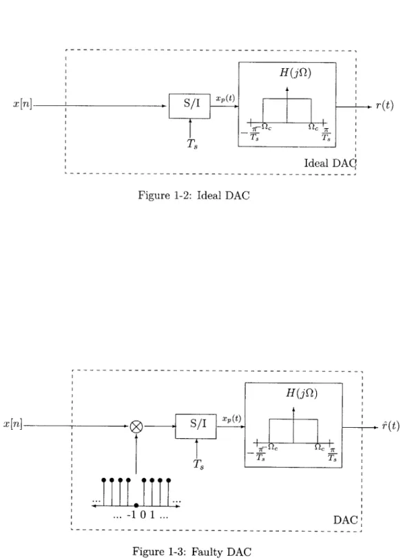
We adhere to the standard mathematical representation for ideal digital-to-analog con-version shown in Figure 1-2. Digital samples, x[n] = x(nT), are converted into an

im-pulse train, xp(t) = __=- x[n]6(t - nT,), through the sample-to-impulses converter (S/I).

xp(t) is then filtered through an ideal low-pass filter (LPF), H(JQ), resulting in the re-construction, r(t). Quantization issues are ignored by assuming that the digital samples, x[n], can be represented with infinite precision. Furthermore, we assume that the original continuous-time (CT) signal, x(t), is at least slightly oversampled. Specifically, we assume that 1/T, = RQc/7r, where x(t) is band-limited to Q, and R > 1 is the oversampling ratio. We denote the ratio wr/R by 7. The DAC perfectly reconstructs x(t) in the sinc basis,

00 _{sin(7r(2Qt - n))}

r(t) = x[n] - -

X(t)

(1.1)

-0 r(2Qct - n

In any practical application, H(jQ) is replaced by a non-ideal filter that approximates the ideal LPF. The choice of H(jQ) will affect our pre-compensation solution, but, for simplicity, we do not consider the effect of non-ideal H(jQ) in this thesis. We assume H(jQ) is always an ideal LPF, with the understanding that in practice it will be approximated accurately enough to meet design specifications.

The faulty DAC is mathematically represented as in Figure 1-3. The dropped sample is modeled as multiplication by (1 - J[n]) that sets x[O] = 0. Without loss of generality, we assume that the dropped sample is at index n = 0 and that the dropped sample is set to

x[n] S/I xr(t)

T-Ideal DA9

Figure 1-2: Ideal DAC

H(jQ) x[n]-

_S/I

r- t)

7rQ c2 7r Ts T TS 1 0 1 ... _DAC:

zero. Because of the dropped sample, the reconstruction, r(t), is a distorted version of the desired reconstruction, r(t).

It is important to note that this problem is not one of data recovery. The sample that is dropped is known exactly inside the digital system. The problem is one of data conversion, the DAC is broken so that a specific sample cannot be used in the reconstruction. The goal is to represent the data differently in the digital domain, so we can achieve the same reconstruction. As such, interpolation and other data recovery techniques are useless.

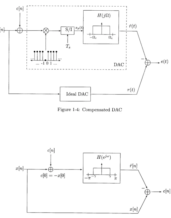
Our goal is to pre-compensate the digital signal x[n], so the distortion caused by dropping

x[O] is reduced. This requires altering samples that are not dropped by the DAC. Figure 1-4

illustrates the compensated DAC. Compensation is portrayed as a signal c[n] that is added to x[n]. In general, compensation could be some complicated function of the dropped sample and neighbors. In our development, we restrict compensation to be an affine transformation of x[n].

We use the squared-L2 energy of the error signal, e(t) = r(t) - i(t), as the error metric

00

6 2 = r(t) - (t)12 dt (1.2)

-00

The problem can be equivalently cast directly in the discrete-time domain as shown in Figure 1-5. In Figure 1-4, we can move the DACs to the right of the summing junction and add a ideal discrete-time LPF, H(eiw), with cutoff y = Q,/T, = 7r/R before the DAC.

The cascade of H(eiw) and the DAC is equivalent to just a DAC, i.e. H(eiw) does not filter any additional energy compared to the DAC. Thus we can move H(esw) left through the summing junction. Since x[n] is band-limited to -y by definition, H(edw) is just a identity transformation on the lower branch, so it can be dropped.

Additionally, there are two places in Figure 1-4 where error enters the system. First from the dropped sample, x[01, and secondly from the compensation signal, c[n]. Tracking the effects of two sources of error is difficult, so to simplify we incorporate the dropped sample into the compensation as a constraint: c[O] = -x[0]. This constraint ensures that

x[0] is zero before entering the DAC, so dropping it does not cause any additional distortion.

Figure 1-5 illustrates our final, simplified representation. We equivalently use the squared-e2

energy of e[n] as the error metric

00

- 20 (1.3)

r~n -- --- - - -- - - - -- --

---e[nl

]_ _ _ _ _ _ H(jQ) x [n] S/I

T

~TS

-.10 1 ... DAC :,.et L - - -_-- - - -_- _-- - - - -_ - -PIdeal DAC -r(t)

Figure 1-4: Compensated DAC

c[n] H(ew)

x[n]

]

c

[0] = - [0]

_l--/

'

e[n]

x[n]

1.2

Constraints

We impose two constraints on digital pre-compensation of the dropped sample. The first, oversampling, is a direct result of the formulation. The second, a symmetric c[n], is imposed for simplification.

1.2.1 Oversampling

In Figure 1-5, the error signal, e[n], can be expressed as

e[n]

x[n]

-

[n]

(1.4)

= x[n]

-

h[n] * (x[n] + c[n])

(1.5)

In the frequency domain

E(ew) = X(eW) - H(ew)X(e3w) - H(elw)C(e3w) (1.6)

Since X(ew) is band-limited inside the passband of H(e3w), (1.6) reduces to

E(eW) = -H(ew)C(ew) (1.7)

Using Parseval's relation, the error E2 reduces to

00

E2

S

emil2 =

I

E(ejw)I2dw (1.8)

J=27r> IH(ejw)C(ew)12dw (1.9)

Minimizing E2 is equivalent to minimizing the energy of C(ei') in the band [--y,-Y],

i.e. in the pass-band of the filter H(ejw). This implies that x(t) must be at least slightly oversampled for compensation.

There are some subtleties involved in this condition. Oversampling is generally defined as x(t) being sampled at a rate 1/T, > 2Q,. This is an open-set, so the limit-point, 1/T. = 2Qc, does not exist in the set. Assuming that x(t) is sampled at exactly 1/T, = 2Qc, there is aliasing at the point w = 7r. In this limiting case, the reconstruction filter, H(ew), can be

chosen to be

H(edW) = 1, w 7r (1.10)

H(eW) = 0, w =7r

It eliminates the aliased point at w = ir, and, since a point has measure zero, there is still perfect reconstruction in the f2 sense. The compensation signal, unless it is an impulse at

W = 7r, will be passed unchanged to the output. Unfortunately, as Section 1.3.2 develops,

choosing c[n] as a properly scaled impulse at w = 7, we can have perfect compensation. So, at least from a formal mathematical viewpoint, we can compensate the limiting case. For this thesis though, we do not consider such measure zero subtleties as they are non-physical. In the limiting case, we assume that the reconstruction filter must be the identity filter defined as

H(eL) = 1 (1.11)

Thus, compensating with impulses will not work and from (1.8), the energy of c[n] is the error.

2 _{C d (1.12)}

In this degenerate case, the optimal solution is to meet the constraint, c[0] =

-x[0],

and set the other values of c[n] = 0, for n 4 0. This is equivalent to having no compensation and letting the faulty DAC drop the sample x[O]. There is no gain in compensating. Proper compensation requires that x(t) be sampled at a rate 1/T, > 2Q,+E, for E 4 0 but otherwise arbitrarily small. We use this as our definition of oversampling. As before, 7r/R = y where

R > 1 is the oversampling ratio with 1/T, = RQc/ir.

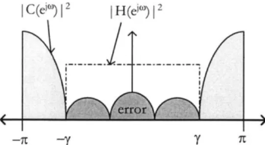
When oversampled according to this definition, X(ew) is band-limited to -y < 7r. As illustrated in Figure 1-6, the reconstruction filter, H(ei") can be designed with a high-frequency stop-band, -y < |w| <7r. c[n] can then be designed such that most of its energy

is in the stop-band of H(ew), minimizing the final error.

In fact, increasing oversampling reduces error even without compensation. The faulty DAC with no compensation can be represented in our simplified model as a degenerate compensation signal

I C(eln)12 1 H(ein)12

Figure 1-6: Oversampling and Compensation

In the frequency domain, C(eiw) is a constant -x[O]. Figure 1-7 illustrates the resulting error. Mathematically, the expression for the error is

E2 = 2-yx2 [0] (1.14)

As the oversampling rate increases, -y decreases, reducing the error accordingly. Intu-itively, oversampling introduces redundancy into the system so dropping one sample con-stitutes a smaller loss of information than if the signal were sampled at the Nyquist rate.

I C(ej,) 12 1 H(ej") 12

Figure 1-7: Error without Compensation

1.2.2 Symmetric Compensation

In general, affine pre-compensation can alter any arbitrary set of samples in x[n]. For clarity in the exposition, we focus on symmetric compensation, where (N - 1)/2 neighboring samples on either side of the dropped sample are altered, i.e. c[n] is a symmetric signal centered around n = 0.

In contexts where the location of the dropped sample is known a priori, such as with missing pixels on a video-display, symmetric compensation is the practical choice. In some

contexts though, symmetric compensation is not feasible. For example, for a DAC that drops samples in a streaming system the best we can do is to detect the dropped samples and compensate causally. The compensation signal will be one-sided and asymmetric. Where the extension to the more general case is obvious, we note the structure of the asymmetric solution.

1.3

Previous Work

This thesis is, in part, an extension of the work done by Russell in [8]. In this section, we review some of the results presented in [8].

1.3.1 Alternative Formulation

The "missing pixel" problem was originally formulated in [8] as a resampling problem. Resampling is the process of converting between two digital representations of an analog signal, each of which is on a different sampling grid. Specifically, in the case of one dropped sample, define an index set I to be the set of integers

I = {0, i1, ±2, ±3, ... }1

and a set I' to be the set of integers with zero removed

I' = {i±1, i2, t3, . .. }

An analog signal x(t) is digitally represented by its samples {Xn} on I. Low-pass filtering the digital sequence {X} through a filter, h(t), reconstructs x(t). The goal of compensation is to find coefficients {X'} on I' which satisfy

x(t) = E

x'h(t

- n) (1.15)

ncI'

or equivalently

x(t) = z'4h(t - n) (1.16)

n=-oo with the constraint

By requiring x' = 0 the sum may be taken over all integers. In this thesis, we take a different viewpoint and pose the problem in the context of DACs. Both formulations are equivalent when h(t) is restricted to be an ideal LPF. The DAC representation is preferred in this thesis because of its practical relevance.

1.3.2 Perfect Compensation

If c[n] had no frequency component outside jwj > 7r - -y while meeting the constraint

c[0] = -x[0], it would perfectly compensate with zero error. There are an unlimited number of signals that meet this criteria. For example, we can simply choose

cif[n] = -x[O](-1)" (1.17)

This signal meets the constraint that cinf [0] = -x[0] and since its spectrum is

-X[0]

C(ew) = [ (6(W - 7r) + 6(W + 7r)) (1.18)

2

C(ew) is completely high-pass, with zero energy in y < jwI < r. cinfrn] perfectly compensates for the dropped sample. This solution only requires in theory that R = I+ 6, where c is non-zero but otherwise arbitrarily small. Russell derives this result in [8] within a resampling framework.

All other perfect compensation solutions are signals band-limited to wj < -y multiplied by ci11 [n]. Of these choices, the minimum energy solution is

csinc[n] = -x[0](-1)n - y)n (1.19)

(7r - Y)n

Unfortunately, all of these signals, although resulting in zero error, have infinite length, making them impractical to implement. Russell in [8] develops an optimal finite-length compensation strategy using constrained minimization. In that spirit, this thesis focuses exclusively on length compensation using perfect compensation and optimal finite-length compensation as a starting point for the more sophisticated algorithms.

1.3.3

Missing Pixel Compensation

In the case of video-displays, the "missing pixel" problem is of practical interest and some ad hoc solutions have been proposed, [6, 4]. In these approaches neighboring pixels are brightened in order to compensate. The idea is based on the fact that the missing pixel looks dark, so making the surrounding pixels brighter reduces the visual distortion. Though several weightings are proposed, no theory is developed.

In [8] Russell implements a two-dimensional version of the optimal finite-length solution and applies it to images with missing pixels, [8]. Since the eye is not an ideal LPF, Russell's algorithm does not perfectly compensate for the missing pixels, but there is a noticeable improvement in perceived image quality. Though such extensions are not considered, the algorithms presented in this thesis can also be extended to two-dimensions for use in missing pixel compensation.

1.4

Thesis Outline

Chapter 2 extends Russell's constrained minimization approach and presents a closed-form solution, referred to as the Constrained Minimization (CM) algorithm. Results from nu-merical simulation are presented. Despite giving the optimal solution, CM is shown to have numerical stability problem for certain parameters.

In Chapter 3, we develop a different approach to the compensation problem by win-dowing the ideal infinite-length solution, cinf [n]. The solution is related to the discrete prolate spheroidal sequences (DPSS), a class of optimally band-limited signals. We develop a DPSS-based compensation algorithm, called the discrete prolate approximation (DPAX). The DPAX solution is shown to be sub-optimal, a first-order approximation to the opti-mal CM solution. However, as we show, DPAX is more numerically stable than CM. As in Chapter 2, results from numerical simulation are presented. In addition, Appendix A presents an interpretation of the DPSS as a singular value decomposition. Appendix B proves duality of certain DPSS.

Chapter 4 presents an iterative algorithm in the class of projection-onto-convex-sets (POCS). The Iterative Minimization (IM) algorithm is proved to converge uniquely to the optimal CM solution. Results from numerical simulation are used to show that the IM algorithm has a slow convergence rate, a common problem for many POCS algorithms.

Chapter 2

Constrained Minimization

In this chapter, we develop constrained minimization as a technique for generating compen-sation signals. Extending the derivations in [8], we derive a closed-form expression for the optimal, finite-length solution called the Constrained Minimization (CM) algorithm. We evaluate the CM algorithm's performance through numerical simulation. Although optimal, CM is shown to have problems of numerical stability.

2.1

Derivation

We closely follow the derivation in [8]. However, our treatment formalizes the constrained minimization using Lagrange multipliers. We assume that the compensation signal, c[n], is non-zero only for n E /V, where A1 is the finite set of points to be adjusted. For simplicity in the presentation, we assume a symmetric form for c[n], i.e. AN= [-N 21,N 2 11, although

the derivation is general for any set PV. Also, for notational convenience, the signals c[n] and x[n] are denoted as the sequences {cn} and {xn}. As shown in Chapter 1,

e[n] = : cnh[n - m] (2.1)

mEK

The error is

00 00

2 - e[n]12 = E ( 1: cmh[n - m])2 (2.2)

n=-oo n=-oo mEJ

Our desire is to minimize 62 subject to the constraint g = co + xo = 0. We do this using the method of Lagrange multipliers. Defining h = E2 - Ag, we minimize h by setting the

partial derivatives with respect to Ck for k E M equal to zero. For Ck 4 Co, & 00 hk

S

2( EcCmh[n - m])h[n - k] = 0 (2.3) ln=-oo _mEN - 2 cm( h[n - m]h[n - k]) (2.4) mEV n=--oo =

ScmEy[k

- m] = 0 (2.5) mCA/

E).,[n]

is the deterministic autocorrelation function of the filter h[n]. The subscript -y denotes the cutoff of the LPF h[n]. Simplifying &,y[n], we obtain

5,[n]

=

h[m]h[n - m] (2.6) m=-oo = h[n] * h[-n] (2.7) sin(yn) - sin(-yn) _(2.8) wrn 7rn sin(yn) h[n] _(2.9) irn

where * denotes convolution. For clarity, we do not replace ),[n] with h[n), despite the fact that they are equivalent. When Ck = co, the derivative has an extra term with A, the Lagrange multiplier.

h =/cEm - n])2 - A(co + =o) 0 (2.10)

&C~J =- 00 \n EJ

= 2 cnE,[-n] - A = 0 (2.11)

nEiV

These derivatives produce N equations. Along with the constraint g, this results in N+1 equations for the N unknown sequence values of cn and the one Lagrange multiplier A. The system, reproduced below, has a unique solution, Copt [n], that is the optimal compensation

signal for the given value of N.

5

cm)[k - m] = 0, k , 0 (2.12)

mEjV

2

5

cmEy[-m] - A = 0, k = 0 (2.13)

We chose [- N= 1, N 1 1] to be symmetric, so the system (2.12), (2.13), (2.14) can be written in block matrix form

2

IK

I

(2.15)

[T

₀

_A

_-Xo

where J is a vector with all zero entries except for a 1 as the center element, i.e.

6T = 0 0 - 0 0 1 0 0

.

0

0

(2.16)

e,

is the autocorrelation matrix for h[n]. Because h[n] is a ideal low-pass filter, E, is a symmetric, Toeplitz matrix with entries

E8(i,

j) = h[i -

i]

= sin. ij (2.17)

7r[i - 3]

The symmetric, Toeplitz structure of

e,

is particularly important in Chapters 3 and 4 in relation to the discrete prolate spheroidal sequences and the iterative-minimization algo-rithm.

To solve (2.15), the matrix 0, must be inverted. We leave a proof of invertibility for Chapter 5. For now, assuming that the inverse exists, (2.15) can be interpreted as two equations

1

En

+ 2 AJ = 0 (2.18)

2

T Cn +

0A

= -xo (2.19)

Combining the two equations,

(

6Te

7

1)

A = -XO (2.20)

6Te

7

16=

,

7

'

((N

1) (N-1)) is the center element of the inverse matrix. For notational

convenience, we choose O1 = 871 ((N 1) (N-1)) The Lagrange multiplier is then

A 2x (2.21)

The optimal compensation signal is

copt[n]

0

(2.22)

oC

1

We refer to the algorithm represented by (2.22) as Constrained Minimization (CM).

2.2

Performance Analysis

2.2.1 Examples

We implemented the CM algorithm in MATLAB and calculated compensation signals for examples in which x[0] = -1. Figure 2-1 shows c0pt [n] and an interpolated DFT, Copt(eiw), using 2048 linearly-interpolated points, for N = 6, N = 10, and N = 20 for -y = 0.97r. Figure 2-2 shows the same for -y = 0.77r.

There are several interesting features to note on these examples. The optimal signal is high-pass as expected. For both cases, the main lobe of the DFT is centered at 7r with smaller side-lobes in the interval [--y, -y]. Furthermore, as N increases, the energy in this low-pass band decreases, thus decreasing the error. Also, we can see that for the same N, the solution for y = 0.77r does better than that of y = 0.97r because there is a larger high-pass band. Intuitively, for smaller y, the system is more oversampled, so a better solution can be found using fewer samples.

c [n] 1 _ _ _ .5 - - - ---. - - -.. . . . - - - . -. 0 .5 -4 -2 0 2 4 5 0 0 .1 -5 0 5 1 IC (evT)l (2048 pts) 0.05 0 .04 - - ---0 .0 3 -.- - .-.-- - .- - .- .- -. - --. -0 .-0 2 --- - - - - ---0.01 -1 -0.5 0 5 1 0.1 0.05 0 -1 -0.5 0 0.5 1 z 0 -0 o z 6 -0 zI F 6 --0 4 3 2 0--1 -0.5 0 0.5 1 Co/ n

Figure 2-1: Optimal sequences c[n] for y = 0.97r and N=7, 11, 21

c 1[n] 1 Q 2 00 - 0 .5 -.-- - - - - -. .--1 -4 -2 0 2 4 1 0.,5 --- .. - ... - ... ---.-- --.

--~L0

-0 .5 - - - -. . .- - . -. - --. --5 0 5 1 cm -0.5 - --10 -5 0 5 10 0.2 0.15 0.1 0.05 0 -1 -0.5 0 0.1 0 0.( 1C (e )| (2048 pts) 0 0.2 0 .15 - - . -.-. -0 .1 -- .. . -.. 0.05 -.- - .- . 01 -1 -0.5 0 (tl/n

Figure 2-2: Optimal sequences c[n] for y = 0.77r and N=7, 11, 21 0. 0. 0. 0. . 5 -. . . . . -. . . . . -. - -.-. - -. -I. ... 1 - 05 -- - -0 -1 -0.5 0 05 0.5 1 05 2

-1 1

2.2.2

Error Performance

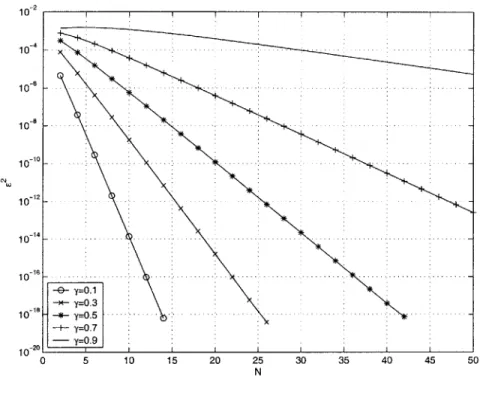
Figure 2-3 illustrates E2 as a function of N for -y = 0.17, 0.37r, 0.57r, 0.77, and 0.97. The graph shows that E2 decreases approximately exponentially in N. Since the CM algorithm generates the optimal solution, the error curves shown in Figure 2-3 serves as a baseline for performance. There is a limited set of parameters -y and N for which the problem is

well-conditioned. Beyond E2 = 10-9, the solution becomes numerically unstable beyond the

precision of MATLAB. 10 15 20 25 N 30 35 40 45 50 Figure 2-3: E2 as a function of N 2.2.3 Computational Complexity

With a direct implementation, using Gaussian elimination, the N x N inversion of e, requires 0(N3) multiplications, and O(N 2) memory, [13]. Exploiting the Toeplitz,

sym-metric structure, we can use a Levinson recursion to find the solution. This does better, using O(N 2) multiplications and O(N) space, [7].

0 5

:y=0.5t :

y=-.7i

i:. n inn~n nn ni i i ::i nEn: i n :ii inK

10-3 10~4 10~5 0-6 10-7 10-8 10-9 10-1 CIIW

2.3

Numerical Stability

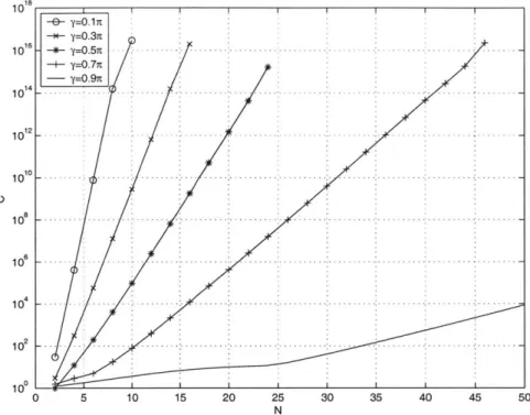
As N increases and -y decreases, the condition number of 0, increases until inversion be-comes unstable. Figure 2-4 plots the condition number of E, as a function of N for various values of -y. The plot shows that the condition number increases approximately exponen-tially. As -y decreases the condition number also increases approximately exponenexponen-tially.

Figure 2-5 shows the condition number as a function in the two-dimensional (N, y) plane. The black region in the lower right-hand corner is where the condition number is reasonable, and the solution is numerically stable. The large semi-circular gray region centered at the upper left-hand corner is where MATLAB returns inaccurate solutions because the problem is too ill-conditioned. The whitish crescent region defines a meta-stable boundary between well-conditioned and ill-conditioned solutions. MATLAB can find accurate solutions for some points in this region, and not for others.

There is only a small region in the plane where the problem is well-conditioned enough for a floating-point implementation of MATLAB to find a solution. Conditioning problems would be even more pronounced in fixed-point DSP systems. Fortunately, the inversion can be done off line on a computer with arbitrarily high precision, since once c0pt [n] is found

it can be stored and retrieved when the algorithm needs to be implemented. Also, in most contexts, an error of 109 = -180dB, compared to the signal, is more than sufficient.

-6-- Y=O. 1 y--0.3n y = 0 .5 n ... .. ... ... .. ... ... ... . ... ... y--0.7n Y=0.9n ... .. .. ... ... ... ... ... . ... ... . . ... ... ... ... ... ... ... . ... ... ... -... ... ... ... ... ... . ... _{... ... ... . ...} .... . . .. ... ... ... ... ... ... ... .... ... ... 0 5 10 15 20 25 30 35 40 45 50 N 10 18 10 16 10" 10 12 10 10 10 8 10 6 i C 102 10 0 now MMM -MMEV MMM ::Mmf.A simOva BMW almm, MMVA Mmvl ' MM"", -w Aa.1n v on;-, raw 0.1 0.2 0.3 0.4 0.5 0.6 0.7 0.8 0.9 Y/n

Chapter 3

Discrete Prolate Approximation

In this chapter, we formulate an alternate approach to the design of finite-length compensa-tion signals based on applying a finite-length window to the infinite length solucompensa-tion, cif [n]. The problem formulation leads us to consider a class of optimally band-limited signals, called discrete prolate spheroidal sequences (DPSS), as windows. An algorithm, which we refer to as the Discrete Prolate Approximation (DPAX) is presented. As the name im-plies, this solution is an approximation to the optimal CM solution using discrete prolate spheroidal sequences. We explore the relationship between DPAX and the CM solution, concluding that the DPAX solution is a first-order approximation of CM in its eigenvector basis. In addition, we evaluate the algorithms performance through numerical simulation. DPAX is shown to be more numerically stable than CM.

3.1

Derivation

3.1.1 Windowing and Discrete Prolate Spheroidal Sequences

With CM, we construct a finite-length compensation signal directly from the imposed con-straints. Alternatively, we can start with the infinite-length signal, cinf[n] = -X[0](-1)n, and truncate it through appropriate windowing. From this perspective, the problem then becomes one of designing a finite-length window, w[n], such that

c[n] = w[n]cif r[n] (3.1)

window design as an optimization problem. C(ejw) = W(eiw) * Ciff(eiw), so we design

w[n] E l2(- N-, N2), to maximize the concentration ratio

fww _"- _ |W(e 12dW

af(N, W) =

W(ew

d

(3.2)

fr,|

IW(ew)1

2

_dW

Slepian, Landau, and Pollak solve this problem in [9, 5, 10] through the development of discrete prolate spheroidal sequences (DPSS). Using variational methods they show that the sequence w[n] that maximizes the concentration satisfies the equation

N-1

2 sin 2W7r[n

_-

_m]

N- _{w[m] =Awn]}

_(3.3)

N-1

= - 2

Expressed in matrix form, the solutions to (3.3) are eigenvectors of the N x N symmetric,

positive-definite, Toeplitz matrix, Ow, with elements

Ow [n, m] =sin 2W(m - n) (3.4)

7r(m - n)

m, n = -(N - 1)/2,... - 1,

0,

1, .... (N - 1)/2

If W = , we obtain

e7,

the same matrix as in Section 3. By the spectral theorem, the eigenvectors, vo [n], are real and orthogonal with associated real, positive eigenvalues, Ar. In addition, in [10] it is shown that these particular eigenvalues are always distinct and can be ordered

A

>

A2 > ...

> AN

These eigenvectors, vW [n], are time-limited versions of discrete prolate spheroidal sequences (DPSS). They form a finite orthonormal basis for (_ N21, N21)j [10].

Note that the DPSS are parametrized by N and W. In cases where there may be

confusion, the DPSS are denoted as iN, W)[n]. This specifies the i-th DPSS for the interval

|nj < N 1 and the band

jwI

< W.

The original concentration problem only requires that (3.3) hold for

InI

< N- 1. By low-pass filtering the time-limited DPSS v) [n], we can extend the range of definition and

thus define the full DPSS

sin 2W7r[m - n]

ui[i] =

Zim

35

M=- m - n]

The ui[n] are defined for all n = (-oc, oc). They are band-limited functions that can be shown to be orthogonal on (-oo, oo) as well as on [-N21, N-21], [10]. They form an

orthonormal basis for the set of band-limited functions e₂(-W, W), [10]. References [10,

9, 5] all comment on this "remarkable" double-orthogonality of the DPSS and its practical importance in applications. In Appendix A we show that this double-orthogonality, and many other properties of the DPSS can be interpreted as the result of the DPSS being a singular value decomposition (SVD) basis.

3.1.2 Extremal Properties of the DPSS

Finally, normalizing the full DPSS to unit energy

Sui

[n]uj[[n] = Jij (3.6)

n=-oo

It follows that

N/2

Z

ui[n]uj[n] =

Aioij

(3.7)

n=-N/2

So the eigenvalue, Aj, is the fraction of energy that lies in the interval [ -1 N 1 ,1[10].

Conversely, normalizing the time-limited DPSS to unit energy

N/2

E vi [n]v [n] = 6_{ij (3.8)}

n=-N/2

It follows that

J Vi(ej)V*(e ')dw = Ajoij (3.9)

The eigenvalue, Aj, in this case, is the fraction of energy in the band fwf < W, [10]. We can

now use the DPSS orthonormal basis to find the answer to our concentration problem. The signal w[n] E f₂, so it has some finite energy E. Expressed in the DPSS basis

with the constraint

al +ce2

+

N

-(3.11)

- --

Our goal is to choose the ai such that the energy in the band 1wI < 7r - -y is maximized. By the orthogonality of {vi[n]}, the energy of w[n] in 1wI < 7r - -y is

aiA1 + a2A2 + +

a2

AN (3.12)

Since there is a constraint on E, in order to maximize the ratio of energy in-band all of the energy should be put onto the first eigenvector, i.e. a, =

V"E

and ai = 0 for i 4 1.

Thus the first DPSS, v1 [n], solves the concentration problem. The maximum concentration

is the eigenvalue, A1. Consequently, the optimal window in our formulation is vi-'[n].

Modulating vVT~~7[n] up to 7r and scaling it to meet the constraint, c[0] -x[0], provides a potential compensation signal

Cdpax [n] x[0] (-1)nvV-[n] (3.13)

vi7 [0]

3.1.3 Duality of DPSS

Every DPSS has a dual symmetric partner. In particular,

V+in]= (-l)nvyrW[i] (3.14)

The eigenvalues are related

+ = A7 W (3.15)

[10] states this property without a detailed proof. We provide a comprehensive proof in Appendix B. Duality implies that the compensation signal, cdpax[n] in (3.13), can also be expressed

V

1[0]N

Cdpaxfl - Nx[0-]

vN

Independent of which DPSS is used to express it, we refer to this solution as the Discrete Prolate Approximation (DPAX). The algorithm above is specific for symmetric compensa-tion. For asymmetric compensation, the solution is also the first DPSS, scaled relative to the dropped sample, v7[k], for k

$

0.

3.2

Relationship to Constrained Minimization Solution

It should be clear that Cdpax [n] is not equivalent to the CM solution, copt [n]. In this section, we illustrate how the window formulation constrains the problem differently, leading to a sub-optimal solution. We also show that the optimal solution is a linear combination of the DPSS. In this context, the DPAX solution is a first-order approximation of the optimal

solution.

3.2.1 Different Constraints

The window formulation starts with a finite-energy signal, optimizes for that energy, and then scales to meet the c[O= -=[] constraint. CM does not begin with an energy con-straint, thus it finds the optimal solution. Specifically, in the CM algorithm, we have a finite set )A on which we design N samples of the signal c[n]. Assume A'= {0, 1}. Two sample values, c[O] and c[1], must be determined. Graphically, as illustrated in Figure 3-1, there exists the (c[O], c[l]) plane on which the error E 2

is defined. The constraint, c[O] = -01, defines a vertical line in the space. The CM algorithm finds the unique point on this line that minimizes E2. This point, copt[n], is the optimal solution given the constraints.

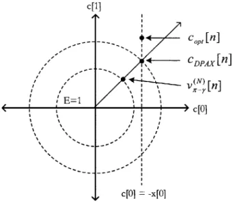
The DPAX solution is fundamentally different. v7,[n], is a signal of unit energy that has minimum error, E2. As illustrated in Figure 3-2, it is the minimum on a circle of radius E = 1 in the (c[0], c[1]) plane. The DPAX algorithm scales v^'[n] to meet the constraint c[O] = -x[O]. Graphically, this amounts to scaling the unit circle until the minimum error point intersects the constraint line c[O] = -x[O]. This point, which is both on the scaled circle and the line, is cdpax [n]. This point is not the same as copt [n]. The DPAX solution is thus sub-optimal for the constraints on the problem.

3.2.2 Constrained Mimimization Solution in the DPSS Basis

The exact relationship between Cdpax [n] and c0opt [n] can be found by decomposing copt [n] in

the DPSS basis, {v7 [n]}. Since

E)

is real and symmetric, it can be diagonalized into its real, orthonormal eigenvector basis which are the time-limited DPSS.

87 = VAVT (3.17)

c[1]

4%

-ct,[n]

C

4 c[0]

c[O]= _-x[O]

Figure 3-1: Constrained Minimization, N = 2

c[1I CCp~lfl co,,[n] E l c[0] C[0 = -x[0

eigenvalues. The inverse, 0-1 is also symmetric and can be diagonalized in the same basis.

6-1 = VA- -VT _-y (3.18)

As proved in [101, the eigenvalues associated with the DPSS are all real, positive, and distinct. Thus, 0, can be diagonalized with non-zero, distinct eigenvalues. The matrix is thus non-singular and can be inverted. c0opt[n] exists, and it can be expressed as

copt[n] - 0 = - '0 VA-VT3 (3.19)

0C1 -Y0 I

01 is the middle element of ₇1, which can be expressed in the DPSS basis as

N

0

1

_A-'

_(V7[o]) 2 _(3.20)

i=(1 Without matrices, copt[n] can be expressed as

copt [n] = - (1A-1vY[n]

+

---

+

A1/NVY[n]) (3.21)

where 3i = v" [0]. The eigenvalues, Aj, are distributed between 0 and 1. The expression for the optimal solution depends on the reciprocals 1/Ai, so the eigenvector with the smallest eigenvalue, vor [n], will dominate. Since scaling this vector produces cdpax[n], DPAX can be interpreted as a first-order approximation to copt[n].

3.3

Performance Analysis

3.3.1 Examples

We implemented the DPAX algorithm in MATLAB and calculated compensation signals in which x[0] = -1. The DPSS were found using the dpss() function in the MATLAB Signal Processing Toolbox. This function computes the eigenvectors of

e,

using a similar, tri-diagonal matrix p-,. The next section, describes the particulars of the implementa-tion. Figure 3-3 shows Cdpax[n] and an interpolated DFT, Cdpax (ei'), using 2048 linearly-interpolated points, for N = 7, N = 11, and N = 21 for y = 0.97r. Figure 3-4 shows the same for -y = 0.77r.

c[n] .5 - - - - -. - . - .-- - .

-0I

.5 - .. . .-. - .- . -. - --. -1 -4 -2 0 2 4 -5 0 5 .5 -.

-0

-10 -5 0 5 10 n |C(e ()|l (2048 pts) 0.2 0.15 -0 .1 - - -. ..- -. . . -.- - ..-0 .0 5 - -. . ..-. . . -.-.-.-.-.-.-0 -1 -0.5 0 0.5 1 0.4 0 .3 - - .- . -. -.-. --.-0 .2 - - - ---0.1 - - - - - -0 -1 -0.5 0 05 1 0.4 0 .3 --- - - - -0 .2 - - - - . . . .- - -. . . -.-.- -. -. 0 .1 - - -- - -.-- - - - .- - .-- -0 -1 -0.5 0 0.5 1 CO/ It

Figure 3-3: DPAX solution c[n] for -y = 0.97r and N=7, 11, 21

c[n] 0 0.5 - -- - - -.-. -. --- . 0 0.5 -1 -4 -2 0 2 4 11 04 1

~L

-0 [.5 -- - - - --5 0 5 1

T

0

L -0 .5 ..-.--- --- -. -. ----.... -10 -5 0 5 10 n IC(e O)I (2048 pts) 0.2 0 .15 - - - - -0 .1 .-- - - - . . . . . . . 0 .0 5 - - -.-.---.-.-.-- - .- 0--1 -0.5 0 05 1 0.2 0 .15 - -- - - - - -0 1 - -- --.-.-.- -.-0.05 - - - -- - - -0 -1 -05 0 05 1 0.2 0 .15 - - - -- - - .. 0 .1 - -.-.- - .-- -0 .05 - - - -.-.-.---0 -1 -0.5 0 0.5 1 OV7I

Figure 3-4: DPAX solution c[n] for y = 0.77r and N=7, 11, 21

0 z 0 2 -0 -0 z 0 Z- -z -0

-Comparing these plots to Figure 2-1 and Figure 2-2 in Chapter 2, we observe that Cdpax[n] looks similar to copt[n]. Like c0 pt[n], Cdpax[n] is harder to band-limit when there

is only a small high-pass band. One noticeable difference is that the zeroth sample is not discontinuous from the rest of the samples like in copt[n]. All of the samples for cdpax[n] can be connected by a smooth continuous envelope.

3.3.2 Error performance

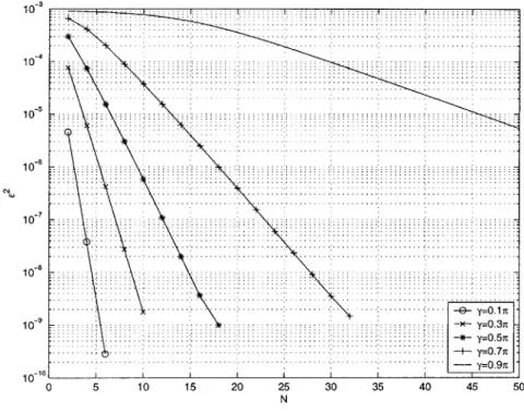
Figure 3-5 illustrates E2 as a function of N for various values of y. DPAX is not as ill-conditioned as CM, so by increasing N it can achieve values of E2 in the range of E2 = 10-20, i.e. about ten orders of magnitude smaller than that using CM.

The DPAX solution is suboptimal compared to the CM solution for the same parameters -y and N. Figure 3.22 plots the gain

2

Ge = dpss (3.22)

Eopt

in error due to DPAX. As the figure illustrates, the gain becomes negligible as N increases and -y decreases. The near-optimal performance of the DPAX solution is explained by the eigenvalue distribution of O7. As N increases and y decreases, the reciprocal of the smallest eigenvalue, 1/AN, increasingly dominates the reciprocals of the other eigenvalues. In (3.21),

v7[n] dominates the other terms, making cdpax[n] a tighter approximation.

Figure 3-7 shows the ratio AN-1/AN as a function of -y for N = 7, N = 11, and N = 21. It illustrates empirically that AN-1 becomes significantly larger than AN as N increases and y decreases. The other eigenvalues A,, A2, etc., are even larger in size. For example, when

N = 21, AN-1 is 250 times larger than AN at -y = 0.57r. Thus in (3.21) the vN) [n term is 250 times more significant than the next order term.

3.3.3 Computational Complexity

The DPAX solution can be computed directly as the last eigenvector of

E8.

Due to the ill-conditioning of

E),

the DPAX solution is better found as the last eigenvector of a similar matrix, p-,. In either case, DPAX requires finding the last eigenvector of a N x N matrix.

Many numerical routines exists for the computation of eigenvectors. For small matrices

50

Figure 3-6: G, = E 2 _{dpSS/E 0}2 pt as a function of N

10-2 10-4 . . . .. . . . . . ... . . . . . . . . .... . . .. . ... . . . .. .. . .. . .. . . . .. . . .. . . . .. . . . .. . . . . .. . . ... . . . . ... .. . . ... . . . ... ... . .... ... . ... . ... ... .. . . .... . . . .. .. . . .. . . . . .. . . . ... . .. . . . .. . . . .. . . .. . . -9- y=O. 1 y=0.3 y=0.5 ... ... ... . y=0.7 Y=0.9 1 10-8 C-4 1 10- 16 10- 18 10-20, 0 5 10 15 20 25 30 35 40 45 50 N Figure 3-5: E 2 as a function of N -6- Y=O. I IE m q y=0.37E Y=0.5TE . ... .. .... .. ... ... . -4- y=0.7Tc Y=O. 87t Y=O. 9TC ... ... ... ... ... ...j ... ... ... . . . .. * ... ... .. ... ... ... ... ... . .... ... ... .. .. .. ... ... .. ... ... ... ... ... ... ... ... . .... 5 10 15 20 1.7 1.6 1.5 C\l 0 1.4 CL Cj 'D_w 1.3 1.2 1.1 1 25 30 35 N 40 45

250 - N=6 N=10 N=20 200 --- - -15 0 - - - - - -- --- ---50- - ... ... ... - ... .... 0 0.5 0.55 0.6 0.65 0.7 0.75 0.8 0.85 0.9 0.95 1 Y

Figure 3-7: Ratio of two smallest eigenvalues: AN1

AN

find all the eigenvectors of a matrix in O(N 2) time, [14].

The DPAX solution only requires calculation of one eigenvector though. As N increases, finding all the eigenvectors of a matrix is wasteful in terms of time and computation. For such cases, the power method for calculating the first eigenvector of a symmetric matrix is well suited for this problem [14]. In particular, the power method can be applied to 8,_, the dual matrix, to find the first eigenvector. By dual symmetry the first DPSS of E,_, multiplied by (-1)" is equivalent to the last DPSS of 9Q. Using the power method, the DPAX algorithm can be implemented more efficiently for larger N.

3.4

Numerical Stability

The ill-conditioning of 81, can be better understood by looking at its eigenstructure. The eigenvalues of 6, correspond to the energy ratio of each of DPSS in band, thus they have values between 0 and 1. Although these eigenvalues can be proved to be distinct, they are usually so clustered around 0 or 1 that they are effectively degenerate when finite machine arithmetic is used. Figure 3-8 shows the distribution of the eigenvalues for N = 11 as a function of y.

This degeneracy is the cause of the ill-conditioning of

e

. This was a problem for the CM algorithm, and is also a problem for the DPAX algorithm. Fortunately, the time-limited DPSS are also solutions of the second order difference equation

1 N-i 1

1rn(N-n)vi[n-1]+[( 1 - )2 _{cos 27rW -xi]vi[n]+- (n+1)(N-1-n)vi[n+1] = 0 (3.23)}

2 2 2

N-i N-i

k , n = _{k~i- 2} 2 ' - 1 0 1 ... ₂2

In matrix form, the solutions to (3.23) are the normalized eigenvectors of a symmetric, tridiagonal matrix py of the form

(N -)2 P~r-YIZ 31N 1 _ )2 cos 2(7r - 7) j = (324 px-~y [i, j] = 2(3.24) (i +1)(N - 1-i) j= i +1 0 otherwise N-i N-i = 2 ' ' '-' 2

The Xi's are the eigenvalues. This equation arises in quantum mechanics when trying to separate the three-dimensional scalar wave equation on a prolate spheroidal coordinate system. This is where the name "prolate spheroidal sequences" originated, [9, 101.

[10] shows that if the eigenvectors of py are sorted according to their respective eigen-values, then they are the same as the ordered eigenvectors of

ey.

The eigenvalues, Xi, are completely different though. Figure 3-9 shows a plot of the eigenvalues as a function of -y for

N = 11. The eigenvalues of py are well spread. In fact, the eigenvalues can be proved to be differ at least by 1, [14]. Accordingly, the DPSS can be computed without any conditioning problems. MATLAB's dpss () function uses this method to find the DPSS.

DPAX is a powerful alternative algorithm to CM. Its performance is nearly optimal, it is less complex, and it has fewer stability problems. The only drawback of DPAX is that for smaller N and large 7, there is a performance loss associated with it. Fortunately, this regime is exactly where the CM algorithm is well-conditioned and feasible to implement.

0.1 0.2 0.3 0.4 0.5 0.6 0.7 0.8 0.9 Y

Figure 3-8: Eigenvalues of

Q,

versus -y for N = 11

0.1 0.2 0.3 0.4 0.5 0.6 0.7 0.8 0.9 1

Y

Figure 3-9: Eigenvalues of py versus -y for N = 11

1 0 0 0 0 -n 0 30 20 10 -10 -20 -30 0 .2 .8 - - --. - .-.- .. .--.--.--. .6 - - - --- -- - - -- - -.4 - - - - -- --- - -- - -.2 - -. -. -. . . .. .. .. . -. .. . . .. . .- -. -.- . . . . 0--.2

-Chapter 4

Iterative Minimization

In this chapter, as an alternative to the two closed-form algorithms, we develop an iterative solution in the class of projection-onto-convex sets (POCS). The algorithm, which we refer to as Iterative Minimization (IM) is proved to uniquely converge to the optimal solution, c0pt[n]. Results from numerical simulation are presented. Empirical evaluation shows that

the IM has a slow convergence rate.

4.1

Derivation

Iterative algorithms are often preferred to direct computation because they are simpler to implement. One common framework for iterative algorithms is projection onto convex sets (POCS). In the POCS framework, iterations are continued projections that eventually converge to a solution that is either a common point in all the sets projected into or, if there are no such points, then points that are the closest between the sets. Detailed background on POCS can be found in [12].

We formulate a POCS algorithm, called Iterative Minimization (IM), that converges to an optimal window, w*[n], that when multiplied by (-1)n gives c0pt[n], the optimal

finite-length solution. It is shown in block diagram form as Figure 4-1. There are three projections in each iteration. Each projection is onto a convex set. A set C is convex if

w = pw1 + (1 -A)w 2 E C (4.1)

Figure 4-1: POCS Representation T B D w(i) -7r+y 0 ,-y -(N-I) -1 0 1 (N-I) 2 2 - - - - - - - - - - - - - - - - - - - - - - - - - - - - - - - - - - - - -P ₀ w(i+l) w[0]=x[O] v w(i+l)

Figure 4-2: Affine Representation

PB w(0 --Tc+y 0 7E-y PD -1 0 1 (N-i) 2 2 x[0] 5[n] 0