Publisher’s version / Version de l'éditeur:
The Proceedings of the Eighteenth (2008) International Offshore and Polar
Engineering Conference: Vancouver, Canada, July 6-11, 2008, 2008-07
READ THESE TERMS AND CONDITIONS CAREFULLY BEFORE USING THIS WEBSITE.
https://nrc-publications.canada.ca/eng/copyright
Vous avez des questions? Nous pouvons vous aider. Pour communiquer directement avec un auteur, consultez la
première page de la revue dans laquelle son article a été publié afin de trouver ses coordonnées. Si vous n’arrivez pas à les repérer, communiquez avec nous à [email protected].
Questions? Contact the NRC Publications Archive team at
[email protected]. If you wish to email the authors directly, please see the first page of the publication for their contact information.
NRC Publications Archive
Archives des publications du CNRC
This publication could be one of several versions: author’s original, accepted manuscript or the publisher’s version. / La version de cette publication peut être l’une des suivantes : la version prépublication de l’auteur, la version acceptée du manuscrit ou la version de l’éditeur.
Access and use of this website and the material on it are subject to the Terms and Conditions set forth at
A global wave energy resource assessment
Cornett, Andrew M.
https://publications-cnrc.canada.ca/fra/droits
L’accès à ce site Web et l’utilisation de son contenu sont assujettis aux conditions présentées dans le site LISEZ CES CONDITIONS ATTENTIVEMENT AVANT D’UTILISER CE SITE WEB.
NRC Publications Record / Notice d'Archives des publications de CNRC:
https://nrc-publications.canada.ca/eng/view/object/?id=fe5760e8-b98d-4add-9022-02e4d584afdb
https://publications-cnrc.canada.ca/fra/voir/objet/?id=fe5760e8-b98d-4add-9022-02e4d584afdb
A GLOBAL WAVE ENERGY RESOURCE ASSESSMENT
Andrew M. Cornett
Canadian Hydraulics Centre, National Research Council Ottawa, Ontario, Canada
ABSTRACT
This paper presents results from an investigation of global wave energy resources derived from analysis of wave climate predictions generated by the WAVEWATCH-III (NWW3) wind-wave model (Tolman, 2002) spanning the 10 year period from 1997 to 2006. The methodology that was followed to obtain these new results is described in detail. The spatial and temporal variations of the global wave energy resource are presented and described. Several parameters to describe and quantify the temporal variation of wave energy resources are presented and discussed. The new results are also validated through comparisons with energy estimates from buoy data and previous studies.
KEYWORDS
: global, wave, energy, power, resource, assessment, analysis, modeling.INTRODUCTION
Global warming, the Kyoto protocol, the depletion of conventional energy reserves and the rising cost of electricity generation have sparked renewed interest in renewable marine energy in many countries. Significant advances in wave energy converters have been made in recent years, and there is a growing realization in many countries, particularly those in Europe, that these technologies will be ready for large scale deployments within the next five to ten years. Despite these exciting developments, the potential wave energy resource in many parts of the world remains poorly defined.
Pontes et al. (1997) observed that since the mid-1980s, numerical wind-wave models had been routinely producing good quality wind-wave estimates and noted that these estimates are of great value for the assessment of offshore wave energy resources. They assessed the performance of two wind-wave models through comparison against buoy data, and selected the WAM model for use in the development of the WERATLAS, an atlas of European offshore wave energy resources. The WERATLAS is described in Pontes (1998). It includes a wide range of annual and seasonal wave climate and wave energy statistics for 85 offshore data points distributed along the Atlantic and Mediterranean European coasts. The statistics result from analysis of outputs from the WAM wind-wave model, and data from several
directional wave buoys. While wave climate predictions for the Northwest Atlantic featured good accuracy, predictions for the Mediterranean and North Seas were less satisfactory.
Barstow et al. (1998) (also Krogstad & Barstow, 1999) obtained estimates of wave energy resources at a few hundred discrete points in deep water along the global coastline based on an analysis of 2 years of satellite altimeter data from the Topex/Poseidon mission (launched in 1992). In this analysis, significant wave heights Hs were obtained from
the altimeter data, while the corresponding wave energy periods Te
required to compute wave power were estimated using a set of direct relationships between significant wave height and energy period. These Hs versus Te curves were obtained from an analysis of buoy
measurements from Norway, Portugal and the South Pacific. On average, one estimate of Hs and the corresponding Te was obtained
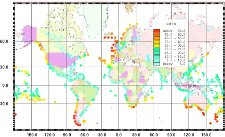
every 5 days over a two year period at several hundred points distributed along the global coastline. Despite the relatively short 2-year record length, the coarse 5-day sampling rate, and the somewhat subjective method of estimating wave energy period, the analysis succeeded in generating reasonable estimates of the spatial variation in mean wave energy off most coastlines. The global wave energy estimates obtained by Barstow et al. (1998) are shown in Figure 1.
Figure 1. Global wave energy estimates from Barstow et al., 1998. More recently, several authors have reported on more detailed wave energy resource assessments for particular regions or countries,
including among others: United Kingdom (ABP-MER, 2004); Ireland (ESBI Environmental Services, 2005); Portugal (Pontes et al., 2005); Canada (Cornett, 2006); California (Wilson and Beyene, 2007); the North Sea (Beels et al., 2007). These types of studies generally involve analysis of wave data from buoys, satellites, numerical wave hindcasts, or a combination of these sources.
Cornett (2006) presents a comprehensive inventory of offshore wave energy resources along the Atlantic and Pacific coasts of Canada, based on analysis of buoy measurements from 68 sites and predictions from three different wind-wave hindcasts:
• a 5-year portion of the AES40 hindcast of the North Atlantic, generated using the OWI-3G model;
• a 3-year hindcast of wave conditions in the eastern North Pacific, generated using the WAVEWATCH-III model; and • a 5-year hindcast of the western North Atlantic generated
using the WAVEWATCH-III model.
Figures were presented illustrating the strong temporal (monthly) and spatial variability of the wave energy resource along both coasts. The wave energy predictions obtained from the wave model outputs were validated through inter-comparison with each other (where possible) and through comparison with buoy data. The accuracy of the wave energy predictions obtained from the wind-wave hindcasts was good for offshore locations, but sometimes less satisfactory for nearshore sites. This must be expected since these wind-wave models could not simulate the complex wave transformations that often occur near the coast.
Despite these developments, the scale and character of the wave energy resource in many regions around the world remains poorly understood and ill defined. The main aim of this paper is to present results from a new analysis of global wave energy resources based on a 10-year prediction of the global wave climate generated by the NWW3-Global wind-wave model. These results may be the best information currently available on the scale, spatial distribution and temporal character of the global wave energy resource.
THEORETICAL BACKGROUND
The energy flux or power (P) transmitted by a regular wave per unit crest width can be written as
g C gH P 2 8 1 ρ = , (1)
where ρ is the fluid density (~1,028 kg/m3), H is the wave height, and
Cg is the group velocity, defined as
T L kh kh Cg ⎟⎟ ⎠ ⎞ ⎜⎜ ⎝ ⎛ + = ) 2 sinh( 2 1 2 1 , (2)
in which h is the local water depth, L is the wave length, T is the wave period, k = 2π/L is the wave number and C = L/T is the wave celerity. The wave length, depth and period are related through the dispersion equation: ) tanh(kh k g T L= . (3)
In shallow water (h < L/2), the following explicit equation for L can be used without noticeable error:
3 / 2 4 / 3 2 2 2 4 tanh 2 ⎪⎭ ⎪ ⎬ ⎫ ⎪⎩ ⎪ ⎨ ⎧ ⎥ ⎥ ⎦ ⎤ ⎢ ⎢ ⎣ ⎡ ⎟⎟ ⎠ ⎞ ⎜⎜ ⎝ ⎛ = gT h gT L π π . (4)
In deep water (h > L/2), C = L/T = 2Cg and L = Lo = gT2/2π, therefore
T H g Po 2 2 32 1 ρ π
= (regular wave in deep water) (5) Real seastates are often described as a summation of a large number of regular waves having different frequencies, amplitudes and directions. The mix of amplitudes, frequencies and directions is often described by a variance spectral density function or 2D wave spectrum S(f,θ). In this case, the power transmitted per unit width can be written as
θ θ ρg π C f hS f dfd P
∫ ∫
g ∞ = 2 0 0 ( , ) ( , ) , (6) with ) tanh( ) 2 sinh( 2 1 2 1 ) , ( kh k g kh kh h f Cg ⎥ ⎦ ⎤ ⎢ ⎣ ⎡ + = , (7)where k(f) is the frequency dependent wave number and h is the local water depth.
The wave power per unit width transmitted by irregular waves can be approximated as ) , ( 16 2 h T C H g P≈ ρ s g e , (8) where Te is known as the energy period and Cg(Te,h) is the group
velocity of a wave with period Te in water depth h. The energy period
of a seastate is defined in terms of spectral moments as
∫ ∫
∫ ∫
∞ ∞ − − = = π π θ θ 2 0 0 2 0 0 1 0 1 ) ( ) ( dfd f S dfd f S f m m Te . (9)In deep water (h > L/2), the approximate expression for wave power transmitted per unit width simplifies further to
2 2 64 e s o TH g P π ρ ≈ . (10)
Measured seastates are often specified in terms of significant wave height Hs and either peak period Tp or mean period Tz. The energy
period Te is rarely specified and must be estimated from other variables
when the spectral shape is unknown. For example, in preparing the Atlas of UK Marine Renewable Energy Resources, it was assumed that Te=1.14Tz (ABP, 2004). Another approach when Tp is known is to
assume
p e T
T =α . (11)
The coefficient α depends on the shape of the wave spectrum: α=0.86 for a Pierson-Moskowitz spectrum, and α increases towards unity with decreasing spectral width. In assessing the wave energy resource in southern New England, Hagerman (2001) assumed that Te=Tp. In this
study, we have adopted the more conservative assumption that α=0.90 or Te=0.9Tp, which is equivalent to assuming a standard JONSWAP
spectrum with a peak enhancement factor of γ=3.3. It is readily acknowledged that this necessary assumption introduces some uncertainty into the resulting wave power estimates, particularly when the real seastate is comprised of multiple wave systems (for example, a local sea plus one or more swells approaching from different directions). However, since P∝TeHs2, errors in period are less
significant than errors in wave height.
NWW3 GLOBAL WAVE MODEL
The Marine Modeling and Analysis Branch (MMAB) of the U.S. National Oceanic and Atmospheric Administration (NOAA) performs continuous operational forecasts of the ocean wave climate around the globe. The wave predictions are performed using a sophisticated third
generation spectral wind-wave model known as NOAA WAVEWATCH III or NWW3 (Tolman, 2002c). The wind fields used to drive the model are obtained from operational products prepared by the U.S. National Centers for Environmental Prediction (NCEP). NWW3 solves the spectral action density balance equation for wave number-direction spectra. The implicit assumption of this equation is that properties of the medium (water depth and current) as well as the wave field itself vary on time and space scales that are much larger than the variation scales of a single wave. A further constraint is that the parameterizations of physical processes included in the model do not address conditions where the waves are strongly depth-limited. These two basic assumptions imply that the model can generally be applied away from the coast on spatial scales (grid increments) larger than 1 to 10 km.
The MMAB has implemented version 2.22 of the NWW3 model on at least six different regular grids, spanning various ocean basins. The NWW3 model and its various implementations have been extensively validated by comparison with data from buoys and satellites. Results of this validation can be viewed in Tolman (2002a, 2002b), and on the Internet at http://polar.ncep.noaa.gov/waves/validation.html.
Results from the Global grid have been used in the present study. The Global grid features a 1.25° by 1.0° resolution and contains 45,216 grid points (29,790 water grid points) spanning the entire globe between latitudes 77°S and 77°N. Unfortunately, the NWW3-Global model does not currently provide wave climate predictions for several important semi-enclosed inland seas including the Mediterranean Sea, the Baltic Sea, Hudson’s Bay and the Red Sea among others. Ice concentrations are obtained from a passive microwave sea ice concentration analysis conducted by NCEP and are updated daily. The minimum depth is 25 m. The effects of sub-grid topographic features (such as atolls, small islands and reefs) are simulated using a pair of obstruction grids which together represent the degree to which wave energy propagation is blocked in each cell.
Due to the 1.25° by 1.0° resolution of the Global grid, processes with fine space scales are not simulated properly. This implies that wave conditions during tropical cyclones, hurricanes and typhoons are not well resolved in the global model. Also, since the grid cannot capture the topographic complexity of most coastlines, and since shallow water effects are not accounted for completely, the model results tend to be less reliable near the coast. As discussed by Pontes et al. (2005), shallow-water wave transformation models and high resolution grids must be used to provide reliable estimates of wave power in coastal waters. Such models are routinely used to provide detailed estimates of nearshore wave climates for coastal engineering studies.
In addition to operational forecasting, the suite of NWW3 models have been applied, using archived wind fields and ice cover charts, to hindcast historical wave fields at 3-hour intervals over several years. The model results (both hindcasts and forecasts) are freely available via the Internet as binary files in GRIB format. The NWW3 wave hindcast results are being used for engineering studies of wave climate around the globe.
ANALYSIS
Data files in binary GRIB format containing results from the NWW3-Global wind-wave model hindcast for a full ten year period between February 1997 and January 2006 were obtained from the MMAB ftp server. These files contained results for the following variables computed at 3 hour intervals for all grid points:
• significant wave height of combined wind waves and swell, Hs
• peak wave period, Tp (period with maximumenergy density)
• primary wave direction, and
• u and v components of the mean 10m wind.
In the presence of ice, both the significant wave height and peak period were set to zero.
Each time series contained 10x365.25x6=21,915 values. The following derived variables were computed for all times at all 29,792 water nodes:
• the wave energy flux (equation (8) with Te=0.9Tp),
• the wind speed; and • the wind power density.
Next, the ten years of data were grouped to form datasets describing conditions annually and during each month and season. Winter was defined to include December, January and February; Spring was defined from March – May; Summer was from June – August and Autumn was from September – November. Then, for every combination of variable, month and season, a set of simple statistics was computed to describe the conditions at every water node. These statistics included the minimum, maximum, mean, standard deviation and root-mean-square values, plus the values corresponding to cumulative probabilities of 10%, 25%, 50%, 75% and 90%. The results were then plotted and further analyzed in various manners.
RESULTS & DISCUSSION
Validation
In order to help verify the wave energy predictions obtained from this analysis, results have been compared with data from several Canadian buoys in the western North Atlantic and the eastern North Pacific. The buoy data is archived and disseminated by the Marine Environmental Data Service of the Department of Fisheries and Oceans, Canada. The analysis of the buoy data has been described previously in Cornett (2005).
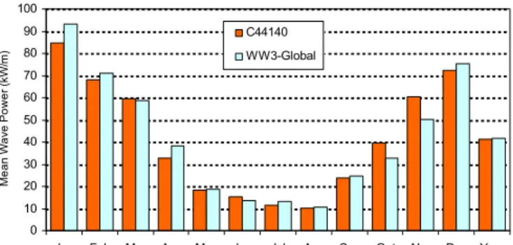
The monthly variation in wave power at buoy C44140, located off the east coast of Canada at +42.73°N,-50.61°W, is shown in Figure 2 together with predictions derived from the NWW3-Global wave climatology for the grid point located at +43°N,-50°W. Both the annual mean power and the monthly power variation are in reasonably good agreement. Recognizing that the two locations are not exactly coincident, the level of agreement is considered satisfactory and sufficient to conclude that the wave energy estimates derived from the NWW3-Global model are reliable.
The monthly variation in wave power at buoy C46184, located off the west coast of Canada at +53.96°N,-138.76°W, is shown in Figure 3 together with predictions derived from the NWW3-Global wave climatology for the grid point located at +54.0°N,-138.75°W. Again, our analysis of the NWW3-Global model results was able to provide a good prediction of both the mean annual wave power and its monthly variation. Similar results were obtained for several other locations in Canadian waters. 0 10 20 30 40 50 60 70 80 90 100
Jan Feb Mar Apr May Jun Jul Aug Sep Oct Nov Dec Year
Me a n W a ve Po w e r (kW /m) C44140 WW3-Global
Figure 2. Monthly mean wave power estimates derived from buoy measurements (station C44140) and WW3-Global wave climatology.
0 20 40 60 80 100 120
Jan Feb Mar Apr May Jun Jul Aug Sep Oct Nov Dec Year
M e a n W a ve Po w e r (kW /m) C46184 WW3-Global
Figure 3. Monthly mean wave power estimates derived from buoy measurements (station C46184) and WW3-Global wave climatology.
Mean Wave Energy Resource
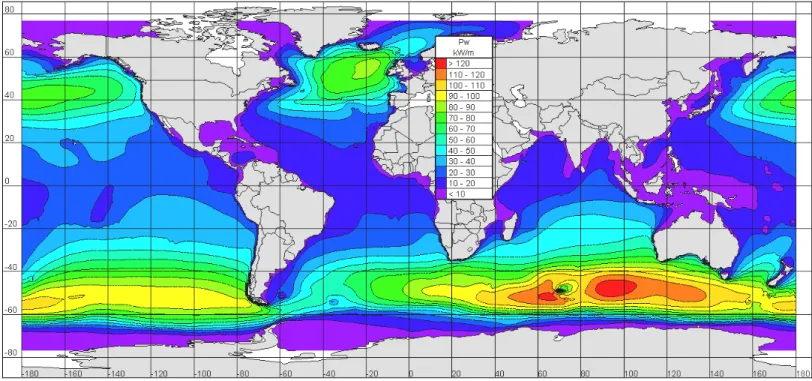
The global distribution of annual mean wave power derived from analysis of the NWW3-Global wave climatology is presented in Figure 4. Equation 8 with Te=0.9Tp was applied to compute the wave power at
all 29,792 water nodes at 3-hour intervals over a 10 year period. Figure 4 presents estimates of wave power for several coastal and many offshore regions that have not previously been considered by other authors.
The resulting spatial distribution of annual mean wave power is generally consistent with both expectations, and with results from previous studies. The annual mean wave power is greatest
• in the higher latitudes of the southern hemisphere (between 40°S and 60°S), particularly in the southern Indian Ocean around the Kerguelen Archipelago and near the southern coasts of Australia, New Zealand , South Africa and Chile; • in the North Atlantic south of Greenland and Iceland and
west of the U.K. and Ireland; and
• in the North Pacific south of the Aleutian Islands and near the west coast of Canada and the U.S. states of Washington and Oregon.
The maximum annual mean wave power in the southern hemisphere is ~125 kW/m, found southwest of Australia near 48°S,94°E. In the northern hemisphere, the annual mean wave power south of Iceland exceeds 80 kW/m around 56°N,19°W, while the maximum in the North Pacific is ~75 kW/m, found near 41°N,174°W.
It is important to note that wave power estimates presented herein describe the energy flux due to wave propagation, and that only a fraction of the energy flux available at any site can be captured and converted into more useful forms of energy. It is also important to recognize that these estimates are less reliable in shallow coastal waters.
Temporal Variability
The variability of the wave energy resource on daily, weekly, monthly and seasonal timescales is a very important factor that will affect the viability of any prospective energy extraction project. Sites with a moderate and steady wave energy flux may well prove to be more attractive than sites where the resource is more energetic, but also unsteady and thus less reliable. Some wave energy converters can be tuned for maximum efficiency in waves with a particular range of periods and heights. Such systems can perform well, with high efficiency, when the prevailing wave conditions remain reasonably steady within this range; however, the system efficiency may decrease significantly when the wave conditions are more variable. Developers may also choose to avoid locations where the extreme wave conditions during storms might damage their energy conversion systems.
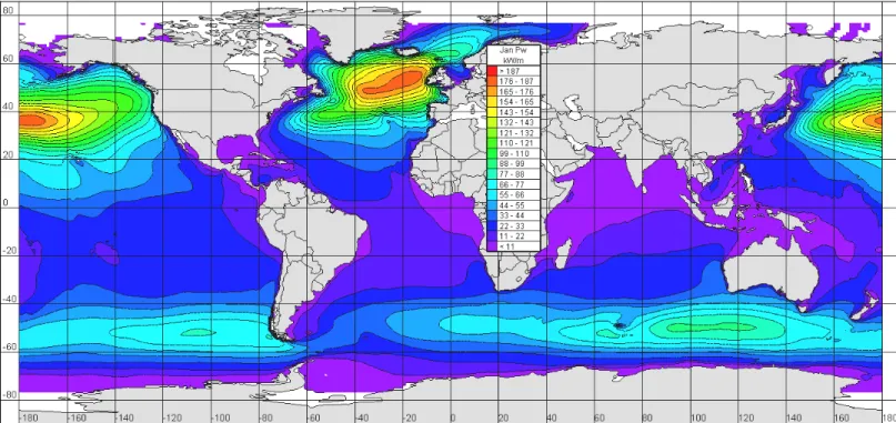
Mean wave power during the months of January and July are plotted in Figure 5 and Figure 6 to illustrate the seasonal variability of the global wave energy resource. During January (Figure 5), most of the world’s wave power is concentrated in the northern hemisphere, whereas during July (Figure 6), the southern hemisphere dominates. The maximum mean wave power during July is ~195 kW/m, found southwest of Australia and east of the Kerguelen Archipelago, near 46°S,91°E. The largest mean wave power in the northern hemisphere during July is ~75 kW/m, found in the Arabian Sea off the coast of Somalia, near 11°N,54°E.
The mean wave power during January reaches ~184 kW/m in the middle of the North Pacific (near 36°N,175°W), and reaches ~182 kW/m in the eastern North Atlantic south of Iceland and west of Ireland (near 54°N,16°W). During January, the mean wave power in the southern hemisphere peaks at ~89 kW/m in the waters south of Western Australia.
It is clear that the wave energy resource at higher latitudes in both hemispheres tends to feature a strong seasonal variability. In contrast, the average level of wave energy in most equatorial regions (between ~25°N and ~25°S) remains more steady throughout the year. The main exception is the Arabian Sea, which is seasonally affected by the Monsoon. Although several semi-equatorial regions are seasonally affected by tropical cyclones, hurricanes and typhoons, the effects of these intermittent storms on time-averaged conditions does not appear significant.
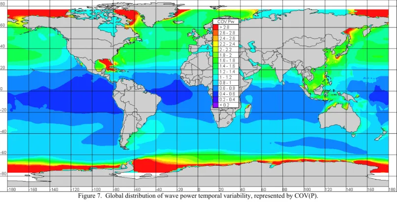
Many measures can be conceived to describe the temporal variability in wave power at a site. One simple, straightforward measure is the coefficient of variation (COV), obtained by dividing the standard deviation of the power time series by the mean power:
( )
P P P t P t P P COV 5 . 0 2 )) ( ( )) ( ( ) ( ⎥ ⎦ ⎤ ⎢ ⎣ ⎡ − = = µ σ ; (12) where σ() denotes the standard deviation, µ() denotes the mean and the over-bar denotes time-averaging. For a normally distributed variable, 68% of the values will fall within the range µ±σ. The coefficient of variation for a fictitious power time series with absolutely no variability will equal zero. COV(P)=1 denotes the case where the standard deviation of the power time series equals the mean value, while COV(P)=2 denotes the case where the standard deviation is twice the mean. The coefficient of variation defined in Eq. 12 measures variability at all time scales, from hourly to seasonal.The global distribution of COV(P), which effectively quantifies the temporal variability of the wave power resource, is presented in Figure 7. These results were obtained from analysis of the NWW3-Global wave climatology every 3 hours over 10 years at 29,792 water grid points as discussed above. As expected, the variability is generally least near the equator in the Atlantic, Pacific and Indian Oceans, with the exception of the Arabian Sea, the Bay of Bengal, and the waters around northern Australia, Indonesia, Malaysia and the Philippines. The global wave power resource is least variable in the eastern Pacific west of the Galapagos Islands, in the western Pacific between Tuvalu and Kiribati, and in the Atlantic near the easternmost coast of Brazil and Fernando de Noronha Island.
The greatest temporal variability occurs in the highest latitudes of both hemispheres where the sea surface is ice-covered for portions of the year. This includes the Beaufort Sea, the Sea of Okhotsk, the northern Bering Sea and the waters around Greenland and Antarctica. These results also indicate that the wave power resource is particularly unsteady in the Gulf of Mexico and the northwestern Caribbean Sea. This may be due to the effects of multiple hurricanes, although further investigation is required to verify this hypothesis.
Near the southern coasts of Chile, South Africa, Tasmania and New Zealand, where the near-coast wave power resource is large, COV(P) values range between 0.85 and 0.9, indicating that the resource is only moderately unsteady. Temporal variability is generally greater in the Northern hemisphere. For example, the following COV(P) values are found for various energy-rich near-coast regions: Ireland (~1.5); Portugal (~1.4); Iceland (1.4-1.6); Norway (1.5-1.6); Newfoundland (1.2-1.4); Vancouver Island (~1.3); Oregon (~1.2); Aleutian Islands (~1.4); Kamchatka (~1.5).
Temporal and seasonal variability of the wave energy resource will be an important consideration affecting any future exploitation of these resources, and therefore should be examined carefully during detailed resource assessments.
Monthly and Seasonal Variability
The concept of a seasonal variability index or seasonality index is proposed to capture, in a single value, a convenient measure of the seasonal variability of the wave energy resource. The Seasonal Variability Index (SV) can be defined as
year S S P P P SV= 1− 4 . (13) Where PS1 is the mean wave power for the most energetic season, and
PS4 is the mean wave power for the least energetic season. For most
parts of the northern hemisphere, winter (December-February) is the most energetic season, while summer (June-August) is least energetic. The SV parameter effectively quantifies the variability of the wave energy resource relative to its mean level on a 3-month seasonal time scale, and is not influenced by variability at shorter time scales. If one assumes that PYear≈½(PS1+PS4), which is reasonably accurate for
many regions, then it is easily shown that
2 / 1 2 / 1 4 1 SV SV P P S S − + ≈ for PS4 > 0. (14)
Eq. 14 provides a simple approximate relation between the Seasonality Index and the ratio of mean wave power during the high and low seasons.
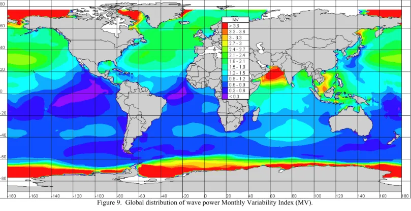
The global distribution of Seasonality Index for wave power is plotted in Figure 8. These results show that the winter-summer seasonal variation (normalized with respect to the yearly mean) is generally greater in the northern hemisphere than in the southern hemisphere. In the near-polar latitudes, the seasonal variability is generally large due to the effects of intermittent ice cover. The largest seasonal variations outside the polar regions occur in the Arabian Sea and in the southern South China Sea. For sites near the west coast of Vancouver Island, the normal range in available wave power between winter and summer is ~1.56 times greater than the annual mean power. According to Eq. 14, this is equivalent to the resource in high season (winter in this case) being ~8 times greater than in low season (summer), which is generally consistent with Figure 3 and previous findings (Cornett, 2005, 2006). It is noted that one can also treat monthly values of mean wave power in a similar fashion to create a Monthly Variability Index defined as
year M M P P P MV= 1− 12 . (15) Where PM1 is the mean wave power for the most energetic month, and
PM12 is the mean wave power for the least energetic month. The
parameter MV describes the maximum range of monthly mean wave power relative to the yearly mean level. For completeness, the global distribution of the Monthly Variability Index for wave power is shown in Figure 9.
Extreme Wave Climate
Some wave energy conversion systems may have difficulty operating successfully in locations that experience extremely large waves on a frequent or even infrequent basis because of the severe technical challenges and/or high costs associated with surviving highly energetic wave conditions.
Hence, many future developers of wave energy projects may seek out locations where the wave energy resource is moderate and fairly steady throughout the year and where the extreme waves are relatively benign. Hence, good, reliable information on the steadiness of the wave energy resource throughout the year and on the severity of the wave climate extremes are important considerations when conducting resource assessments or scouting locations for wave energy projects.
The maximum significant wave height over a 10-year period provides a decent measure of the severity of a wave climate. Figure 10 shows the global distribution of maximum 10-year significant wave height predicted by the WW3-Global climatology. Readers are cautioned against using these results for engineering design, since the extreme wave heights may be under-predicted in some locations due to certain limitations of NWW3-Global model previously mentioned, and the fact that a proper extreme value analysis has not been undertaken. Nonetheless, these values provide a handy general indication of wave climate extremes in various regions. As noted previously, the intensity and frequency of severe wave conditions will likely be an important factor influencing future attempts at wave energy resource development.
CONCLUSIONS
A new analysis of the global wave energy resource has been presented, derived from analysis of wave climate predictions produced by version 2.22 of the NWW3-Global wind-wave model. The NWW3 model has been well-validated and calibrated through extensive comparison against buoy and satellite data. Except for a few semi-enclosed inland seas, the new results provide full global coverage from 77°S to 77°N. The new results have been validated through comparison with buoy data in the western North Atlantic and the eastern North Pacific, and through comparison with results from several regional studies. These results may provide a better account of the scale and character of the global wave energy resource than was previously available.
The temporal variability of the global wave energy resource has been investigated and new measures have been proposed to quantify this important property. The Seasonal Variability Index (SV) and the Monthly Variability Index (MV) are proposed as new parameters that are easy to compute and serve to quantify the seasonal and monthly variability of the wave energy resource. The coefficient of variation of wave power is proposed to quantify the wave power variability at short, medium and long time scales. Finally, the global distribution of 10-year maximum significant wave height is included to provide a general indication of wave climate severity in various regions.
The amount of available wave power, the steadiness of this supply, and the frequency and intensity of extreme wave conditions are all important factors influencing the sitting of wave energy projects. The new results presented here provide a comprehensive global overview of these properties.
ACKNOWLEDGMENT
The writer thanks all reviewers for their helpful suggestions. The NWW3 hindcast data utilized in this study are in the public domain and were obtained through the NOAA-MMAB website. The buoy data referenced in this work were obtained through the website of DFO-MEDS. My colleague Ji Zhang assisted with the analyses described
herein and his efforts are acknowledged with sincere thanks. This study was partially supported by funding from Natural Resources Canada, and this support is gratefully acknowledged.
REFERENCES
ABP Marine Environmental Research Ltd. (2004) Atlas of UK Marine Renewable Energy Resources: Technical Report, Report No. R.1106 prepared for the UK Department of Trade and Industry. Barstow, S., Haug, O. and Krogstad, H. (1998) Satellite Altimeter Data
in Wave Energy Studies. Proc. Waves’97, ASCE, vol. 2, pp. 339-354.
Beels, C., Henriques, J., De Rouck, J., Pontes, M., De Backer, G., Verhaeghe, H. (2007) Wave Energy Resource in the North Sea. Proc. 7th EWTEC, Porto, Portugal.
Cornett, A.M. (2005) Towards a Canadian Atlas of Renewable Ocean Energy. Proc. Canadian Coastal Conference 2005. Dartmouth, N.S., November.
Cornett, A.M. (2006) Inventory of Canada’s Offshore Wave Energy Resources. Proc. 25th International Conference on Offshore Mechanics and Arctic Engineering. Hamburg, Germany.
ESBI Environmental Services (2005) Accessible Wave Energy Resource Atlas: Ireland: 2005. Report No. 4D404A-R2 prepared for the Marine Institute / Sustainable Energy Ireland.
Hagerman, G., 2001. Southern New England Wave Energy Resource Potential. Proc. Building Energy 2001, Boston, USA.
Krogstad, H. and Barstow, S. (1999) Satellite Wave Measurements for Coastal Engineering Applications. Coastal Engineering 37: 283-307.
Pontes, M.T., (1998) Assessing the European Wave Energy Resource. J. Offshore Mechanics and Arctic Engineering, vol. 120, pp 226-231.
Pontes, M., Barstow, S., Bertotti, L., Cavaleri, L., Oliveira-Pires, H. (1997) Use of Numerical Wind-Wave Models for Assessment of the Offshore Wave Energy Resource. J. Offshore Mechanics and Arctic Engineering, vol. 119, pp 184-190.
Pontes, M., Aguiar, R., Oliveira-Pires, H., 2005. The Nearshore Wave Energy Resource in Portugal. J. Offshore Mechanics and Offshore Engineering. Vol 127-3, pp 249-255.
Tolman, H. L., 2002a: Validation of WAVEWATCH III version 1.15 for a global domain. NOAA / NWS / NCEP / OMB Technical Note Nr. 213, 33 pp.
Tolman, H.L., 2002b: Testing of WAVEWATCH III version 2.22 in NCEP's NWW3 ocean wave model suite. NOAA / NWS / NCEP / OMB Technical Note Nr. 214, 99 pp.
Tolman, H.L., 2002c. User Manual and System Documentation for WAVEWATCH-III version 2.22. NOAA-NCEP-MMAB Technical Note 222. U.S. Department of Commerce, Washington, D.C. Wilson J. and Beyene, A. (2007) California Wave Energy Resource
Evaluation. J. Coastal Research. vol. 23-3, pp. 679-690
Figure 5. Global distribution of mean wave power during January.
Figure 7. Global distribution of wave power temporal variability, represented by COV(P).
Figure 9. Global distribution of wave power Monthly Variability Index (MV).