Advanced modeling ,control, and design of an electromechanical engine value drive system with a limited-angle actuator

(1)

Advanced Modeling, Control, and Design of an Electromechanical

Engine Valve Drive System with a Limited-Angle Actuator

by Yihui Qiu

Submitted to the Department of Electrical Engineering and Computer Science in partial fulfillment of the requirements for the degree of

Doctor of Philosophy at the

MASSACHUSETTS INSTITUTE OF TECHNOLOGY February 2009

Author………...…. Department of Electrical Engineering and Computer Science

January 9, 2009

Certified by………..…. John G. Kassakian Professor, Electrical Engineering and Computer Science Thesis Supervisor

Certified by………...…. Thomas A. Keim Principal Research Engineer, Laboratory for Electromagnetic and Electronic Systems Thesis Supervisor

Accepted by………..……. Terry P. Orlando Chairman, Department Committee on Graduate Students

(2)

(3)

Advanced Modeling, Control, and Design of an Electromechanical

Engine Valve Drive System with a Limited-Angle Actuator

by Yihui Qiu

Submitted to the Department of Electrical Engineering and Computer Science on February 2009, in partial fulfillment of the

requirements for the degree of Doctor of Philosophy

Abstract

This thesis addresses a specific variable valve actuation (VVA) system ---- an electromechanical valvetrain ---- in order to provide variable valve timing (VVT) in internal combustion (IC) engines. This electromechanical valve drive (EMV) system was proposed by Dr. Woo Sok Chang and his colleagues in the Laboratory for Electromagnetic and Electronic Systems (LEES), who also validated the feasibility of the design to provide VVT. The goal of this thesis is to bring the MIT EMV system to a more practical level by achieving a smaller package (to fit in the limited space over the engine head), a faster transition time (to accommodate faster engine speed), and a lower power consumption, while still offering satisfactory valve transitions with timing control. This thesis reports four major achievements.

First, a more accurate system model, including dynamics, loss flow and distributions, and nonlinear friction, has been established for better guidance in system control and design via numerical simulations.

Second, different control strategies and cam designs have been explored in order to determine the most appropriate control strategy and cam design to achieve a lower torque requirement, reduced power consumption and a faster transition time.

Third, a limited-angle actuator was custom designed and built for the valve actuation application in order to reduce the actuator size while maintaining the necessary torque and power output.

Fourth, with the limited-angle actuator in place, the EMV system was evaluated experimentally for intake valve actuation and numerically for exhaust valve actuation with gas force disturbance taken into consideration. Based on this system evaluation, we are able to project the system’s applicability to a real 4-cylinder 16-valve engine with independent valve control for each intake and exhaust valve.

(4)

At the end of the thesis, the power consumption has been reduced from 140 W to 50 W (about 64%), the transition time has been reduced from 3.3 ms to 2.7 ms, and the final actuator volume has been reduced to 1/7 of that of the original motor. These significant improvements enabled the projection of independent valve actuation for a 4-cylinder 16-valve IC engine with reasonable power consumption and high engine speed.

Thesis Committee:

Prof. John G. Kassakian (co-supervisor)

Professor of Electrical Engineering and Computer Science Dr. Thomas A. Keim (co-supervisor)

Principal Research Engineer of Laboratory for Electromagnetic and Electronic Systems Prof. David J. Perreault (Thesis reader)

Associate Professor of Electrical Engineering and Computer Science Prof. Wai K. Cheng (Thesis reader)

(5)

Acknowledgments

First of all, I would like to thank my committee members. I am extremely grateful to my co-supervisors Prof. John Kassakian and Dr. Thomas Keim for their constant guidance, patience, support, and understanding during these six and half years. I would not be at this position without their tremendous help. I owe great gratitude to Prof. David Perreault, who has constantly devoted his precious time, brilliant ideas, and strong support to my project. I deeply appreciate Prof. Wai Cheng’s agreement to be my committee member and offer valuable opinions from an engine expert’s point of view. I also want to thank my former colleagues who worked on this project. Dr. Woo Sok Chang, Dr. Tushar Parlikar, Mr. Michael Seeman, Mr. Fergus Hurley, Mr. James Otten, and Mr. Ryan Slaughter, whose work has been very meaningful and helpful to my thesis research.

I also want to extend my sincere thanks to the whole LEES, including professors, staff, and students, who are always there when I need their help.

Prof. Zahn generously gave me the Maxwell® license so I could use Maxwell® in my research; Prof. Leeb has always been patient whenever I bugged him from time to time to borrow all kinds of instruments; Prof. Kirtley, my RQE committee member, helped me learn a lot about permanent magnets and motor design; Prof. Lang was very kind to help me to find an appropriate storage place of epoxy related product and also offered me a TA position when I had a funding problem; Prof. Schindall, another RQE committee member of mine, offered great ideas during our discussion on the project; and Prof. Verghese, also actively helped me to find a TA position so I could be supported financially.

And speaking of LEES staff, Wayne, Vivian, Dave (Otten), Gary, Dimonika, Makiko, Miwa, Kiyomi, Karen, thank you all for your tremendous support for my project and thank you for the wonderful times, too.

My fellow graduate students in LEES, Warit, Riccardo, Yehui, Jiankang, Bernard, Natalija, Kevin, Steve, Tony, Jackie, Robert, Al, and the list goes on and on, thank you all for being around, being supportive, being available when I needed some help, or needed somebody to share excitements or frustrations.

Special thanks goes to the EECS graduate office staffs, who have been taking care of all the trivial stuff so I can focus on my research and class work; Dr. James Bales from the MIT Edgerton Center, who generously lent me the high speed camera and patiently trained me on how to use it; GWG of MIT and GW6 of EECS which offered me a place where I could share my academic and personal experiences with my fellow women graduate students; Mr. William Beck of the MIT Plasma Science and Fusion Center, who offered excellent suggestions on armature fabrication and also gave me many samples of fiber glass sleeves for this purpose; Peter, Andrew, Mike, and other staff of the MIT machine shop, who helped me build and assemble the actuator; Mr. George Yundt and

(6)

Mr. Bill Fejes of Danaher Motion Corporation, who shared with us some great thoughts on motion control; The Ford Motor Company and the Eaton Corporation for their donation of a conventional valvetrain each; and The Industrial Technology Research Institute of Taiwan for their half-year financial support and technical cooperation.

This project was mainly funded by the Sheila and Emanuel Landsman Foundation and the Herbert R Stewart Memorial Fund.

And last but not the least, I owe my family the deepest gratitude. My parents and my brothers back in China, my husband, my mother-in-law and my two-year-old son here in Boston, all have been extremely supportive and understanding in their own way along this long journey of mine at MIT. I wouldn’t be where I am without their backing me up with substantial and irreplaceable love.

This thesis would not be possible to finish without the help and support from all the people I mentioned above. Thank you all so very much.

(7)

List of Illustrations

Fig. 2.1. The Pischinger EMV system [20]. ... 25

Fig. 2.2. The MIT EMV system [19]... 27

Fig. 3.1. A desirable transfer characteristic for the NMT... 31

Fig. 3.2. The whole EMV system [20]. ... 34

Fig. 3.3. Front view of the system including motor and spring assembly [20]. ... 35

Fig. 3.4. The nonlinear mechanical transformer [17]. ... 36

Fig. 3.5. Three operation modes of engine valve motion [17]... 37

Fig. 3.6. Block diagram of the closed-looped EMV system... 38

Fig. 3.7. Experimental results for the initial mode [19]... 40

Fig. 3.8. Rotor and valve position profiles during transition mode. ... 41

Fig. 3.9. Current profile during transition mode... 42

Fig. 4.1. Loss flow of the EMV system. ... 48

Fig. 4.2. Experiment 1 --- 4 V dc input directly to the motor... 49

Fig. 4.3. Experiment 2 --- 0 A current command to motor drive... 50

Fig. 4.4. Experiment 3 --- 5 A current command to motor drive... 50

Fig. 4.5. The design parameters of the NMT... 53

Fig. 4.6. Summary of the EMV system scheme. ... 55

Fig. 4.7. Latest version of the EMV system schematic in 20-sim®. ... 61

Fig. 4.8. Position and current profiles in 20-sim® simulation... 62

Fig. 4.9. Friction and winding loss tracking in 20-sim®_{simulation. ... 62}

Fig. 4.10. Open-loop experiments to extract friction coefficients. ... 63

Fig. 4.11. Simulation results of initial mode... 64

Fig. 4.12. Experimental results of initial mode... 64

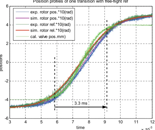
Fig. 4.13. Position profiles of transition mode from experiment and simulation. ... 65

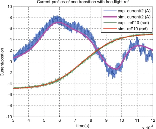
Fig. 4.14. Current profiles of transition mode from experiment and simulation... 65

Fig. 4.15. Comparison of current and previous friction models. ... 66

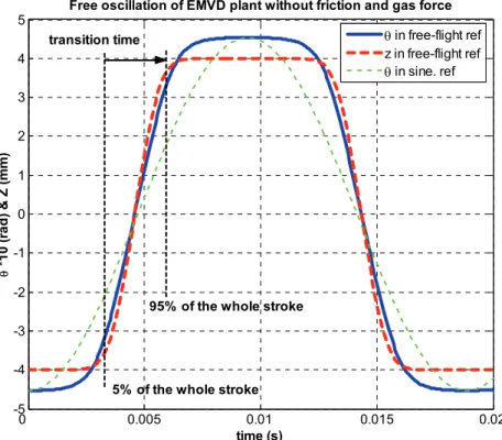
Fig. 5.1. Free-flight trajectory of the EMV system from simulation... 70

Fig. 5.2. Sim. and exp. position profiles with free-flight position reference. ... 71

(12)

Fig. 5.4. Sim. results with free-flight position reference, no current limit. ... 73

Fig. 5.5. Sim. results with free-flight position reference, 8 A current limit. ... 73

Fig. 5.6. Rotor and valve position profiles from experiment with 8 A limit. ... 74

Fig. 5.7. Current profile from experiment with 8 A limit. ... 74

Fig. 5.8. Position profiles with the kick off and capture strategy. ... 77

Fig. 5.9. Current profile with the kick off and capture strategy... 77

Fig. 5.10. Position profiles with 8 A kick off current pulse... 78

Fig. 5.11. Current profile with 8 A kick off current pulse... 78

Fig. 5.12. Position profiles with 5 A kick off current pulse... 80

Fig. 5.13. Current profile with 5 A kick off current pulse... 80

Fig. 5.14. Position profiles with pure open-loop control. ... 83

Fig. 5.15. Current profile with pure open-loop control... 83

Fig. 6.1. Different modulus functions... 93

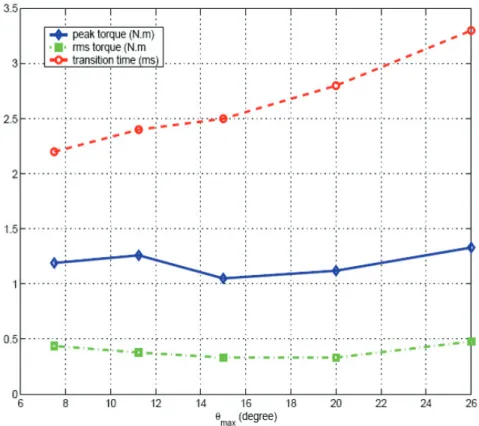
Fig. 6.2. Peak torque, rms torque, and transition time as a function of θ-range... 98

Fig. 6.3. Important physical parameters in a cam design... 99

Fig. 6.4. Roller trajectory with h=16.75mm and o 26 max = θ in the x-y plane. ... 100

Fig. 6.5. Roller trajectory with h=16.75mm and ₂₀o max = θ in the x-y plane. ... 101

Fig. 6.6. Roller trajectory with h=16.75mm and o 15 max = θ in the x-y plane... 102

Fig. 6.7. Roller trajectory with h=28.75mm and ₁₅o max = θ in the x-y plane. ... 102

Fig. 6.8. Roller trajectory with h=28.75mm, o 15 max = θ , mmL_e =2 in the x-y plane.103 Fig. 6.9. Final design of the new _±₁₅o_{cam... 103}

Fig. 6.10. Position profiles with new cam and pure closed-loop control... 106

Fig. 6.11. Current profile with new cam and pure closed-loop control. ... 106

Fig. 6.12. Sequential improvements in power consumption... 108

Fig. 6.13. Sequential improvements in peak torque requirement. ... 108

Fig. 6.14. Sequential improvements in transition time. ... 108

Fig. 6.15. The intake valve, the brush dc motor, and the new brushless dc motor... 109

Fig. 6.16. Position profiles with the brushless dc motor... 110

(13)

Fig. 6.19. Modulus characteristics of a promising 4-bar linkage design. ... 114

Fig. 6.20. Conceptual design of a promising 4-bar linkage. ... 114

Fig. 7.1. Topology I of a limited-angle actuator... 120

Fig. 7.2. Topology II of a limited-angle actuator... 120

Fig. 7.3. Topology III of a limited-angle actuator. ... 121

Fig. 7.4. Topology IV of a limited-angle actuator. ... 121

Fig. 7.5. Topology V of a limited-angle actuator. ... 122

Fig. 7.6. Conceptual design of the moving armature... 124

Fig. 7.7. Another conceptual design of the moving armature... 124

Fig. 7.8. A closer look of the active portion of the armature... 125

Fig. 7.9. Nominal topology with geometric parameters labeled... 128

Fig. 7.10. Optimal dimensions for the limited-angle actuator. ... 129

Fig. 7.11. Size comparison of the limited-angle actuator and the dc brushless motor. .. 131

Fig. 7.12. Simulation profiles with the limited-angle actuator. ... 132

Fig. 7.13. Back-to-back transitions with current pulses of ± 125 A. ... 134

Fig. 7.14. Back-to-back transitions with 98% lift and current pulses of ± 160 A. ... 134

Fig. 7.15. Different rotor positions for torque output. ... 135

Fig. 8.1. Mold to make the armature... 140

Fig. 8.2. Armature-shaft structure... 141

Fig. 8.3. Insulation pattern 1. ... 142

Fig. 8.8. All mold parts with mold release coatings. ... 144

Fig. 8.9. Picture of all materials prepared for winding process. ... 145

Fig. 8.10. Picture of the winding in mold with hose clamps put on. ... 146

Fig. 8.11. Picture of the end turns in desired positions... 147

Fig. 8.12. Picture of the end turns impregnated with epoxy... 148

Fig. 8.13. Picture of the armature structure before curing... 148

(14)

Fig. 8.15. SolidWorks® model and picture of the armature with only mold part 2. ... 150

Fig. 8.16. SolidWorks® model and picture of the cured armature structure w/o shaft. .. 150

Fig. 8.17. Three-layer and five-piece design of the iron yoke... 151

Fig. 8.18. Modified core 3 to accommodate ball bearing to support shaft. ... 152

Fig. 8.19. Permanent magnets and magnet spacers. ... 153

Fig. 8.20. Shaft and core 1 modification for encoder installation... 154

Fig. 8.21. Assembling of core 3, core spacers and magnet spacers... 154

Fig. 8.22. Assembling with permanent magnets added. ... 155

Fig. 8.23. The first two steps of assembling the armature and partial core. ... 155

Fig. 8.24. The last two steps of assembling the armature. ... 156

Fig. 8.25. Core 2 and core 3 added to the partial stator assembling. ... 156

Fig. 8.26. Core 1 installed completing the stator assembling. ... 156

Fig. 8.27. The encoder installed on the actuator... 157

Fig. 8.28. The fully assembled limited-angle actuator... 157

Fig. 9.1. The cylinder for testing the inner armature diameter. ... 160

Fig. 9.2. Relation between the width of the armature and its angular range. ... 161

Fig. 9.3. The end-to-end distance of the armature. ... 161

Fig. 9.4. Two different insulation patterns... 162

Fig. 9.5. Schematic of dc static test of actuator torque constant... 166

Fig. 9.6. Fitting the simulated and experimental free-flight trajectory... 168

Fig. 9.7. Simulation with the measured actuator parameters... 169

Fig. 9.8. The experimental setup with the limited-angle actuator. ... 170

Fig. 9.9. The old L-shaped and the new U-shaped valve holders... 171

Fig. 9.10. The drive used for the limited-angle actuator... 172

Fig. 9.11. 50 ns dead time before increasing C1 and C2. ... 173

Fig. 9.12. 125 ns dead time after increasing C1 and C2. ... 173

Fig. 9.13. Experimental results with 75 A, 6.5 ms current command. ... 175

Fig. 9.14. Experimental results with 60 A, 9 ms current command. ... 175

Fig. 9.15. Gas force versus valve position @ 6000 rpm... 177

Fig. 9.16. Simulation of exhaust valve opening transition with gas force... 177

(15)

Fig. 9.18. Position and current profiles of exhaust valve opening w/o gas force. ... 180

Fig. 9.19. Position and current profiles of exhaust valve opening against gas force... 180

Fig. 9.20. SolidWorks® illustration of the EMV system mounted on an engine head. .. 181

Fig. A1.1. The tangent angleα at the contact point. ... 189

Fig. A1.2. Upper surface, lower surface, and center trajectory of the cam slot... 190

Fig. A1.3. The coordination and cam parameters to estimate cos(α). ... 191

Fig. A1.4. The plot of cos(α) vs. θ of the old cam... 194

Fig. A1.5. The plot of cos(α) vs. θ of the new cam. ... 195

Fig. A2.2. 15-degree disk cam. ... 200

Fig. A2.4. Middle layer of iron core for the actuator... 202

Fig. A2.5. Inner layer of iron core for the actuator... 203

Fig. A2.6. Magnet spacers for the actuator... 204

Fig. A2.7. Core spacer for the actuator... 205

Fig. A2.8. Mold part 1 for the armature making... 206

Fig. A2.12. Inner clamp for the armature. ... 210

Fig. A2.13. Outer clamp for the armature... 211

Fig. A2.14. Shaft for the armature and actuator. ... 212

Fig. A2.15. Cap to connect the stator to the stationary part of the encoder... 213

Fig. A2.16. Supporting part 1 for the actuator... 214

Fig. A2.17. Supporting part 2 for the actuator... 215

Fig. A2.18. Four threaded holes added to column 1 [18] for the actuator support... 216

Fig. A3.1. Simulation schematic with pure closed-loop control... 219

Fig. A3.2. Modulus generator for the nonlinear transformer... 220

Fig. A3.3. Sinusoidal position reference generator... 221

Fig. A3.4. Free-flight position reference generator. ... 222

Fig. A3.5. Lead compensator plus current clamper. ... 223

Fig. A3.6. Simulation schematic with combination control. ... 224

(16)

Fig. A6.1. Pure closed-loop control with sinusoidal position reference... 237 Fig. A6.2. Combination control with free-flight position reference and initial pulse. ... 238 Fig. A6.3. Pure open-loop control with a current pulse... 239

(17)

List of Tables

Table 3.1. Preliminary experimental results. ... 43

Table 4.1. Simulation parameters of intake valve actuation... 56

Table 5.1. Torque requirements w/ and w/o current limit from simulation... 75

Table 5.2. Performance comparison with different control strategies and cams. ... 84

Table 5.3. Ac loss w/ or w/o extra inductor in zero current command experiments. ... 85

Table 5.4. Power consumption w/ or w/o extra inductor in one transition... 86

Table 6.1. Comparison of the old cam and the new cam designs... 104

Table 6.2. Comparison of system performance with the new cam and old cam. ... 107

Table 6.3. Performance comparison with brush and brushless dc motor. ... 111

Table 7.1. Design objectives of the actuator... 117

Table 7.2. Comparison of different topologies of the limited-angle actuator... 122

Table 7.3. Defined physical dimensions of the limited-angle actuator... 127

Table 7.4. Torque output and winding inductance with different vertical air gaps. ... 130

Table 7.5. Final physical dimensions of the limited-angle actuator. ... 130

Table 7.6. Comparison of two commercial motors and the limited-angle actuator... 133

Table 7.7. Torque output at different temperatures and rotor positions. ... 136

Table 7.8. Comparison of winding loss at different temperatures... 137

Table 9.1. Summary of the armature dimensions. ... 161

Table 9.2. Comparison of two insulation patterns. ... 163

Table 9.3. Armature Resistance ... 164

Table 9.4. Armature Inductance with air core or iron core... 164

Table 9.5. The torque constant of the actuator... 166

Table 9.6. Extracted mechanical actuator parameters. ... 167

Table 9.7. Comparison of the new and old simulation. ... 168

Table 9.8. Summary of the transition time and power distribution. ... 176

Table 9.9. Combined exp. and Sim. results for a complete EMV actuation system... 178

Table 9.10. Specification of ITRI’s 2.2 L engine (for one cylinder) ... 179

(18)

(19)

C

HAPTER

1 I

NTRODUCTION

1.1 Introduction

Energy challenges and environmental pollutions are becoming more and more serious problems in today’s world. Automobiles, which consume oil and output emissions, are an important contribution to these two critical problems. People have been actively seeking solutions to minimize oil consumption and exhaust emission of automobiles via different ways for decades. The research work can be roughly summarized in two directions. One direction is to give up partially or totally the current internal combustion (IC) engine, as in hybrid cars. The other direction is to stay with the internal combustion engine but try to optimize its performance under any load and speed condition via advanced control and design techniques. This thesis addresses a specific IC engine improvement ---- an electromechanical valvetrain.

As early as a few decades ago, people recognized that despite the simple design and low cost of conventional crankshaft-synchronized cam driven valve actuation, it can offer optimized engine performance at only one point on the engine torque-speed operating map. Commonly, valve lift profile and timing are chosen to give good performance of high load and high speed, in part because such a choice gives reasonable engine operation over much of the engine map. But at load conditions away from high speed and high load, other valve strategies, were they achievable, might offer reasonable engine performance with better fuel economy or lower emissions, or both.

In particular, research has shown that variable valve timing can achieve significant improvements including fuel efficiency, emissions, torque output, and other possible benefits. As a result, many new types of variable valve actuation have been proposed and studied. However, commercialization of those techniques has been difficult for many reasons, which will be discussed in more detail in Chapter 2. Based on the study of previous proposals for variable valve actuation, a novel electromechanical valve drive (EMV) system was proposed by a group of MIT researchers several years ago. As will

(20)

become evident shortly, the fundamental contribution of the MIT EMV system is the flexibility to separately control the starting timing of valve opening and closing events. We call this capability variable valve timing (VVT). This novel system also introduced a deliberately non-linear element called a nonlinear mechanical transformer (NMT) in order to achieve inherent soft landing and zero power consumption between valve transitions. Feasibility of the concept has been validated by previous work [18]. Further enhancement of the system performance in several practical aspects via advanced modeling, control, and design will be the main focus of this thesis.

1.2 Thesis Goals

The objective of this research is to bring the proposed MIT EMV system to a more practical level by achieving a smaller package (to fit in the limited space over the engine head), a faster transition time (to accommodate faster engine speed), and a lower power consumption, while still offering satisfactory valve transitions with timing control.

The objective is described in more detail below:

1. To establish a more accurate nonlinear system model of the EMV system to help with more effective system dynamic analysis;

2. To model and simulate the EMV system, including the mechanical structure and electrical components, by using a simulation software package (20-sim®) as a platform for better control and design decisions;

3. To evaluate different control strategies by simulations and experiments in order to decrease torque requirement and power consumption of the actuator;

4. To study the possibility of obtaining an optimal design of the nonlinear mechanical transformer, which will offer a lower torque and power requirement and a faster transition;

(21)

5. To propose a novel actuator design customized for the application --- a limited-angle actuator --- which is able to provide satisfactory VVT function and is small enough to fit into the limited space on an engine head;

6. To design a limited-angle actuator using 3-dimensional design software SolidWorks® before building and assembling the actuator;

7. To evaluate the EMV system with the custom designed actuator by simulations and by experiments and confirm the benefits of the proposed system with experimental results;

8. To introduce gas force into the simulation for the case of an exhaust valve and confirm with simulation results the feasibility of the EMV system with the limited-angle actuator in this case;

9. To predict a full picture of variable valve actuation (VVA) for both intake and exhaust valve of a real engine before offering some insights on possible future work.

1.3 Thesis Organization

This thesis is organized as follows:

In Chapter 2, the background and motivation of this project is presented. The starting point of this thesis, i.e., the proposed EMV system and the preliminary experimental results, will be reviewed in Chapter 3. Chapter 4 will discuss the dynamic model, loss structure, and nonlinear friction model of the system developed here. The evolution of the simulation structure of the EMV system will also be described. With the help of the more advanced system modeling, different control strategies are described and improved experimental results are obtained in Chapter 5. Also, relying on numerical simulations

(22)

based on the effective system modeling, Chapter 6 targets an optimal design of the NMT and confirms the expected advancement of system performance through experiments. A novel actuator design customized for the application, a limited-angle actuator, is proposed and analyzed in Chapter 7, while the practical design and fabrication of the actuator are discussed in Chapter 8. Chapter 9 presents experimental evaluation of the EMV system with the new limited-angle actuator, and projects performance of full VVA of a 4-cylinder 16-valve engine based on both experimental and simulation results. Finally, Chapter 10 concludes the thesis and offers some perspectives on possible future work.

(23)

C

HAPTER

2 B

ACKGROUND AND

M

OTIVATION

This Chapter provides more detailed background on VVT and VVA. Several different approaches to realize VVA will be reviewed and compared. Emphasis is placed on electromechanical valve drive systems, including the Pischinger EMV system [9] and the MIT EMV system [17]. The motivation behind this project will be obvious at the end of this chapter.

2.2 VVT

After many decades of continuous development, researchers are still trying to get even better engine performance out of IC engines. Higher fuel efficiency and lower exhaust emissions have always been on the top of the most important goals and are becoming more urgent and critical objectives lately due to the increase of automobile usage, the rapid consumption of the limited oil source, and the increasingly severe pollution of the atmosphere. VVT is one of the most promising emerging technologies in support of the evolution towards better engine performance [1]-[3]. To some extent, electromechanical variable valve actuation can be seen as the ultimate solution to achieving infinite adjustability of valve timing, as will be discussed in this and the following sections [4].

In conventional IC engines, the valves are actuated by cams that are located on a belt- or chain-driven camshaft. As a long developed valve drive, the system has a simple structure, low cost, and offers smooth valve motion. However, the valve timing of the traditional valvetrain is fixed with respect to the crankshaft angle because the position profile of the valve is determined purely by the shape of the cam. Meanwhile, the valve timing desired at different load conditions and speeds could be very different in order to increase torque/power output, minimize fuel consumption, and reduce exhaust emissions. In other words, a cam that idles well with clean emissions typically can't generate much power at high speed, while another high-power cam design will have more emissions at

(24)

idle and be balky at low speed. As a result of the inherent compromises in cam design, the optimal engine performance with one cam design is only possible at certain operating conditions (traditionally at high speed, wide-open throttle and full load conditions) [1]. If instead, the valve timing can be decoupled from the crankshaft angle and can be adjusted adaptively for different situations, then the engine performance can be optimized with respect to higher torque/power output, increased gas mileage, and reduced emissions, at any point of the engine map. This flexibly controlled valve timing is called variable valve timing and the corresponding valve drive system is called variable valve actuation. From the research of engine scientists, the main benefits from variable valve timing can be summarized in specific numbers: a fuel economy improvement of approximately 5~20%, a torque improvement of 5~13%, an emission reduction of 5 ~10% in HC, and 40~60% in NOx [1]-[7]. Other possible gains include enabling a smaller starter/battery, a

combined starter/alternator and the replacement or elimination of many mechanical components.

2.3 VVA

To achieve VVT, substantial research on different kinds of engine valve actuation has been done. There are three main categories: pure mechanical [6], [8], [12], electro-hydraulic [1], and electromechanical valve drives [4], [9]-[16].

The various mechanical actuators are mainly improved designs based on the current valvetrain. One basic type is to switch between two completely different cam profiles [6]. Another popular drive changes valve timing by advancing and retarding one set of cams, while the valve duration stays the same [8]. Both concepts are simple and widely accepted as effective valve drives. But the control flexibility is still very limited and discrete, compared to the ultimate goal of continuously adjusted valve timing of both phase and duration, plus individual control of each valve in order to achieve single valve/cylinder deactivation/activation and engine idle at low speeds.

(25)

The electro-hydraulic device, on the other hand, offers much more flexibility in terms of VVT control. But the use of a hydraulic system makes it expensive and cumbersome, compromising its practicality for automobile manufacture.

The concept of electromechanical actuation has become more feasible and attractive recently owing to its simple structure, continuous VVT control, and independent action for each valve and each cylinder. Although there are several different approaches to electrify the original mechanical valve drive, the bi-positional electromechanical valve drive (BPVD, also referred to as the Pischinger EMV system) has become a popular research topic and has gotten closest to real engine application [9]-[16]. As shown in Fig. 2.1, the Pischinger EMV system, proposed by Pischinger et. al. [9], consists of two normal force actuators and a spring-valve system.

Fig. 2.1. The Pischinger EMV system [20].

The springs are introduced into the system in order to provide the large force needed for valve acceleration and deceleration during each transition. The force requirements of the actuator are thereby substantially reduced. The normal force actuator can only exert an attracting force to the armature. It cannot repel the armature. The force constant of the normal force actuator is proportional to the inverse of the square of the air gap between the active actuator and the armature connected to the valve stem. In other words, the

(26)

force constant is small at the beginning of the transition but is very large when reaching the end of the transition. The good side of these features is that only a very small current will be needed to hold the valve at either the closed or open position due to the large force constant at the end of each transition. However, the down side of the large and unidirectional force constant turns out to be the difficulty of achieving soft landing when the valve is approaching the valve seat. Soft landing, i.e., low valve seating velocity, at the end of each transition, is very critical in terms of acoustic noise and lifespan of the valves. This situation could be more severe in the presence of a high gas force, as will occur with an exhaust valve. In recent literature, soft landing has been achieved by a complicated nonlinear control scheme under certain circumstances [14][15]. However, the impact of gas force disturbance has yet been taken into consideration.

As discussed above, the main cause of the landing problem in the Pischinger EMV system is that the normal force actuators are unidirectional actuators with a nonuniform and nonlinear force constant versus valve position. To solve this problem, Dr. Woo Sok Chang and his colleagues proposed a new type of electromechanical valve drive [17], referred to hereafter as the MIT EMV system. This MIT EMV system inherits the valve-spring system and its regenerative benefits from the Pischinger EMV system, while using a bi-directional shear force actuator with a uniform torque constant. As shown in Fig. 2.2, the motor shaft is connected to the valve system via a nonlinear mechanical transformer (NMT). Inherent soft landing is guaranteed by a special design of the NMT, as will be discussed in Chapter 3. The experimental results of the first prototype proved the feasibility of the system up to 6000 rpm engine speed, as also will be reviewed in Chapter 3.

2.4 Motivation of Further Research

Although Dr. Chang and his colleagues have shown some exciting results, there still are several challenges that need to be addressed in order to put the proposed system into a real engine.

(27)

Motor

Z

θ _CamDisk

Z θ

Side view

Front view

Roller

Fig. 2.2. The MIT EMV system [19].

One of the most important challenges is size: the motor used in the first prototype was far too big compared to the limited space over the engine head, considering that there are 16 valves on a modern four cylinder engine and independent control over each valve is preferred. Another challenge is to lower the electrical power consumption of the system. A third issue regards the transition time. It is very desirable to achieve a faster transition time since modern IC engines are pursuing higher and higher engine speed where 6000 rpm is not high enough anymore. Last but not least, the gas force has not been taken into consideration yet. This needs to be addressed especially for the case of an exhaust valve.

(28)

(29)

C

HAPTER

3 T

HE

P

ROPOSED

EMV S

YSTEM

This chapter reviews the MIT EMV system originally proposed by Dr. Woo Sok Chang et. al. [17], starting by explaining the basic concept and discussing the prominent features of the system mainly owing to the nonlinear mechanical transformer (NMT). Then the preliminary control scheme, the initial design of the nonlinear mechanical transformer, and the first prototype are described. Finally, the preliminary experimental results are studied, which not only prove the feasibility of the idea, but also offer valuable insights on directions for future research. All of the analytical and experimental work of the proposed EMV system reported in sections 3.2 to 3.4, and essentially all of the interpretation thereof, are the work of Dr. Woo Sok Chang and his colleagues Tushar Parlikar and Michael Seeman [17]-[21]. The author of this thesis joined the MIT EMV research group at August 2002 just in time to observe and then conduct the preliminary experiments and process experimental data afterwards. Section 3.5 summarizes the author’s observations and thoughts on how to improve the EMV system performance for the purpose of this thesis.

3.2 Basic Concept of the MIT EMV System

In order to solve the problems associated with the previously discussed VVT systems, a new EMV system was proposed by Dr. Woo Sok Chang and his colleagues, who were members of MIT’s Laboratory for Electromagnetic and Electronic Systems (LEES) [17]-[18]. This EMV system comprises an electric motor that is coupled to a resonant valve spring system via a NMT. As already shown in Fig. 2.2. The NMT is implemented by a slotted cam connected to a motor shaft and roller follower which in turn is connected to the valve stem via a valve holder. It is straightforward to see how this device works based on Fig. 2.2. When the motor swings back and forth within the angle range limited by the cam slot design, the roller follower moves back and forth within the slotted cam, allowing

(30)

the valve to move up and down between fully open and fully closed positions. Note that the angular range of motor rotation, i.e., the angular range of the cam slot, is a design parameter of this system, while the full stroke of the valve usually will be determined by engine design.

In the proposed EMV system, the shear force motor acts as a uniform–force–constant and bi-directional actuator, through which the valve timing is controlled and the friction force and gas force during transitions are overcome. Compared to the Pischinger EMV system [9], which uses two normal force actuators, this design allows valve transition in two opposite directions via one control channel.

For the same reason described when discussing the Pischinger EMV system, a pair of springs is introduced into this system to offer the large force needed to accelerate and decelerate the valve mass and rotor inertia during each transition. In other words, the springs store and regenerate the kinetic energy (transferring between potential energy in the springs and kinetic energy in the valve) as the valve moves between the two ends of the stroke, which will sharply reduce the power and torque requirements of the motor. The two springs are identical, so the equilibrium point of the springs is designed to be the middle position of a full stroke, i.e., half-open position.

The mechanical transformer is responsible for transferring the rotation of the rotor into the translation of the valve in a desired way. In particular, we desire to achieve small seating velocity of the valve at the end of each transition, zero holding power/torque when the valve needs to stay at fully open or closed positions, and reduced peak torque and hence rms torque requirements of the motor. In order to accomplish these goals, a NMT with a z−θ characteristic like that is shown in Fig. 3.1, is designed and will be discussed in the next section.

(31)

3.3 Prominent Features Due to the NMT

This section will describe the merits of using a NMT, in terms of at least four aspects. More details on the idea of MIT EMV system with a shear force actuator, a spring valve assembly, and a NMT can be found in Dr. Woo Sok Chang’s PhD thesis [17] and other publications on the MIT EMV system [18]-[20].

-30 -20 -10 0 10 20 30 -5 -4 -3 -2 -1 0 1 2 3 4 5

θ

(degree)

z (mm)

Fully open position

Fully closed position

Fig. 3.1. A desirable transfer characteristic for the NMT.

For the valve-spring system, the spring forces are the largest at the ends of the stroke because the spring forces increase linearly with valve displacement from the middle of the stroke. If the relationship between valve motion and motor shaft motion were linear, these large spring forces would make it difficult to hold the valve in the open or closed position without using a large motor torque, and thus substantial electrical power. The same issue will arise when we try to open the exhaust valve, where, under some engine conditions, the large gas force will be at its peak at the beginning of the transition. With a linear mechanical transformer, a much larger starting torque, and hence a much larger peak/rms torque of the motor are required to complete the transition. The high torque and power requirements will result in the need for large-size motor as well as reduced fuel

(32)

efficiency of the engine. In addition, precise control of the valve seating velocity would require precise control of the motor velocity, which would impose exacting standards on control. A cam profile such as that in Fig. 3.1 allows all these problems to be solved, as we will show below.

Let us define the displacement of the rotor as θ and that of the valve as z , then obviously θ is a function of z and vice-versa. Assume that the NMT implies the following relation between θ and z ,

) (θ g z= _(3.1) dt d d dg dt dz θ θ ⋅ = (3.2) 2 2 2 2 2 2 2 d d d d d d d d d d t g t g t z θ θ θ θ ⎟⎠ + ⎞ ⎜ ⎝ ⎛ = (3.3)

Assume the nonlinear mechanical transformer provides an ideal coupling between the z-domain and the θ -z-domain, that is to say, there is no power loss or energy storage inside the coupling. Therefore we can equate the power in the z and θ domains as shown in (3.4) and obtain the following relations as shown in (3.5) by using the NMT characteristic as shown in (3.2): dt dz F dt d z⋅ = ⋅ θ τ_θ (3.4) z F d dg θ τ_θ = (3.5)

where τ_θ is the torque in the θ -domain and F_z is the force in the z-domain.

There are essential benefits obtained by using this nonlinear mechanical transformer. At either end of the stroke, the slope of the cam characteristic

θ

d dg

is designed to be very

close to zero, as shown in Fig. 3.1. Thus, the reflected motor inertia in the z-domain is very large, creating inherently smooth valve kinematics profiles since the valve is slowed

(33)

it easier to control the motor velocity near the ends of the stroke in the sense that possible high rotation speed and hence overshoot in the θ -domain will not prevent small seating velocity of the valve at the end of each transition. Also, overshoot of the rotor is allowed by extending the flat slope area in the θ -domain. Moreover, the large spring forces at the ends of the stroke in the z-domain are transformed into small torques in the θ -domain, also due to the flat end of the transformer. Therefore static friction is enough to hold the valve at open or closed positions without any power or torque input from the motor. This is a big energy saver for the engine, especially at lower speed conditions where the valve spends much more time at closed or open positions than in a transition. In addition, because the gas force on the exhaust valve is largest at the beginning of the opening transition, the reflected gas force obtained in the θ -domain is also small, making it easier to open the exhaust valve against a large gas force. Compared to the linear case, the peak torque is both reduced in magnitude and delayed until later in the transition.

In summary, the nonlinear design of the transformer which has flat ends will ensure an inherent soft landing, allow some overshoot of the motor, realize zero torque/power valve holding, and reduce peak torque and hence the rms torque requirements of the motor.

3.4 Preliminary Experimental Results

In this section we will present the first prototype setup and the control scheme used to obtain the first satisfactory transition. Then the experimental results of that transition are discussed [17]-[20].

3.4.1 First Prototype Setup

In order to prove the concept of the proposed EMV system, an experimental apparatus was designed, constructed, and integrated into a computer-controlled experimental test stand, which is hereafter referred as our first prototype.

The test stand consists of a computer-controlled digital signal processor (DSP) board (the DS1104 from dSPACE, Novi, MI), a motor drive, a shear-force motor with an optical

(34)

shaft angle encoder, a valve-spring assembly, and a disk cam and roller follower to implement the NMT. The dSPACE control board is used to receive the shaft angle feedback signal, to process the signal to implement the controller transfer function, and also to generate the output current/torque command. It is supported by software that allows us to construct the input and output terminals and controller in a MATLAB® SIMULINK® file before compiling and to conveniently implement the whole structure on the DSP board. The motor drive is used to receive a current/torque command and inject the desired amount of current into the motor, which then will initiate and complete a valve transition with the help of the springs. An oscilloscope is used to record position, current, and voltage information. These data can be acquired to a .txt file by Labview® for later computational analysis. The whole setup is shown in Fig. 3.2 [20] as below. More details on the setup design can be found in Dr. Tushar Parlikar’s Master’s degree thesis [18]. Steel Table PC with Simulink and dSPACE Control Desk Oscilloscope EMVD Apparatus Motor Drive Power Supplies DSP I/O Channel Motor

Fig. 3.2. The whole EMV system [20].

An off-the-shelf permanent magnet dc motor (the 4N63-100 from Pacific Scientific, Rockford, IL), as shown in Fig. 3.2, was picked for our preliminary evaluation because it

(35)

power consumption, appropriate speed rating, good electrical and mechanical time constants, and so on. However, this motor is large in size --- too large to fit into the limited space over the engine head. Therefore even though this motor proves the concept of the MIT EMV system, a much smaller motor will be required to practically implement the proposed EMV system, which is one main target of this thesis.

To achieve the intended control system bandwidth, a high-bandwidth motor drive circuit realizing hysteretic current control has been developed; details of this design can be found in [21].

To meet the transition time requirement of no less than 3.5 ms for 6000 rpm engine speed, a pair of die springs having the appropriate stiffness (56 kN/m) were selected based on the known valve mass, rotor inertia, and disk cam inertia [17]. A pair of these springs was used together with a standard exhaust engine valve from a 16 valve, 2.0 L Ford Zetec® cylinder head to form a valve-spring assembly, as shown in Fig. 3.3.

Linear Position Sensor Bottom Plate Top Plate Disk Cam Roller follower Valve Seat Spring Spring Divider L-shaped Valve Holder Motor Shaft

(36)

A differential optical encoder with an 8192-line resolution (E6D from US Digital, Vancouver, WA) was selected for rotary position sensing.

The disk cam is one of the most important parts in this EMV system due to its nonlinear characteristics as discussed in the previous section. To realize the zero-slope design at both ends of the stroke, a sinusoidal function with an effective rotation range of ±26

degrees was initially chosen to fulfill the desired NMT characteristics. A few extra degrees are added at both ends to extend the flat end to allow overshoot of the rotor without affecting the finishing positions of the valve. The designed NMT part is shown in Fig. 3.4. The desired NMT characteristics within the effective angular range and the extended flat range are given by (3.6) and (3.7) respectively,

z= f(θ)=4sin(3.46θ) mm θ ≤26°,or,0.454 rad (3.6) mm ) ( 4 ) (θ signθ f z= = ⋅ θ ≥26 or°, ,0.454 rad (3.7)

Fig. 3.4. The nonlinear mechanical transformer [17].

3.4.2 Operation Modes and Control Schemes

The operation of the EMV system can be separated into three modes: initial, transition and holding. In the initial mode, the valve is moved from its resting position (the middle

(37)

of the stroke) to one end of the stroke (closed or open). Friction will keep a resting valve firmly at the open or closed end of a stroke, even in the absence of an electromagnetic holding torque. It may be possible to manage engine shutdown in such a way that all the valves are parked either closed or open, as is more appropriate for the subsequent engine-starting event. If this is possible, the initial mode may not be used often, if ever.

The valve is moved from one end of the stroke to the other end during the transition mode within a limited time and with a small seating velocity. Both initial mode and transition mode are followed by the holding mode during which the valve is held at the arrival end with a variable holding time. The three modes are illustrated in Fig. 3.5 [17]. Two different control schemes were designed for these three modes: one was designed to realize both transition and holding mode by shaping the reference input appropriately, while the other was designed to carry out initial mode control.

Closed Open Initial mode Holding mode Transition mode time Valve position (z)

Fig. 3.5. Three operation modes of engine valve motion [17].

• Transition Mode Control

During the transition mode, the valve is driven between the fully closed and fully open positions. Thus a position feedback control strategy was chosen when we were trying to evaluate the system via simulations and experiments. Because the motor is the control

(38)

unit in the system and the valve position is rigidly related to the rotor position via the NMT, the rotor position θ was chosen to be the feedback variable and control target. Currently, an optical encoder is used to detect the rotor position. A block diagram of the closed-looped EMV system is shown in Fig. 3.6. The EMV plant is comprised of the motor drive, motor, NMT, and the valve-spring system. The reference position input is a position trajectory, which includes the desired starting and finishing motor positions, corresponding to the valve starting and finishing positions respectively. The reference trajectory, a half cycle of a sinusoidal signal for simplicity here, is chosen with proper frequency in order to achieve the desired transition time. The system output is actual motor position detected by the position sensor. The difference between the actual motor position and the reference position is passed into a controller, which provides a current control input to the motor drive. The motor drive then supplies the desired current to the motor. Reference Generator Controller Motor Drive Motor Rotor Position Sensor Nonlinear Mechanical Transformer Valve Spring System Gas Force Disturbance

Control signal connection

Mechanical connection Power signal connection

In cylinder gas force

+

-

_x

Fig. 3.6. Block diagram of the closed-looped EMV system.

In practice, a fixed-gain lead compensator was used for our first try to obtain a successful transition measured by transition time and seating velocity, as will be presented in section 3.4.3. The transfer function of the lead compensator is given by (3.8) [17],

(39)

P S Z S K S G / 1 / 1 ) ( + + = (3.8)

where K is the controller gain, Z is the zero location of the lead compensator, and P is

the pole location of the compensator. The selection of the three constants is discussed in more detail in [17] and [18].

The objective of the holding mode is to hold the valve at either end of the stroke for a controllable time. This control of holding mode was combined into transition mode control by shaping the reference input to stay constant when it reaches the maximum position in either direction, using the same control law as for the transition mode. After the motor has been observed to be motionless at the end positions, zero current control is implemented. The presence of flats at the ends or of near-flat conditions near the ends is enough to overcome the spring force attempting to initiate a transition. It would be relatively simple to introduce small detents for “parking” if necessary, but that is not treated here.

• Initial Mode Control

As discussed above, the initial mode control may be valuable if we want to move the valve from its equilibrium position to either end position before engine start-up after a failed valve transition. To avoid requiring the motor to overcome the full static force of the springs, we drive the system at its resonant frequency by applying a series of current/torque pulses to the EMV system until the valve reaches the desired end position. During this process, the sign of the current/torque pulses will be flipped when the motor/valve velocity changes its sign. When the valve is close enough to the desired end position, the system switches to transition mode control to assure a soft valve landing.

The control law of the initial mode is given by (3.9) [17]:

ω ω α⋅ / =

i _(3.9)

where i is the current command sent to the motor and motor drive, ω is the nonzero

angular velocity of the motor and α is a pre-determined constant. In a discrete implementation, i keeps its previous value whenever ω =0.

(40)

3.4.3 Preliminary Experimental Results

As discussed in section 3.4.1, a single-valve experimental apparatus was designed and constructed in order to validate that the proposed EMV system is technically feasible for up to 6000 rpm engine speed. A simple closed-loop control is used, as shown in section 3.4.2, where the displacement in the θ -domain is the control target. Based on previous hardware and software implementation, we now present and discuss some preliminary experimental results [17]-[20].

• Initial Mode Behavior

As shown in Fig. 3.7, the initial mode is completed within 35 ms with 8 A current pulses, which is sufficiently fast for practical applications. The average power during the initial mode period is approximately 150 W [17], which is acceptable since this is a one-time operation.

(41)

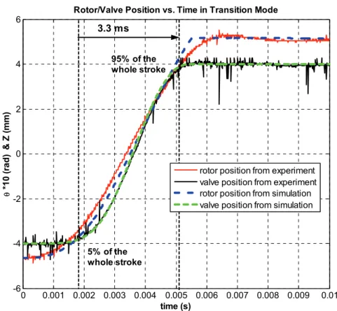
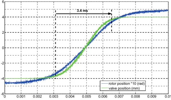
When the valve was sufficiently close to the desired end, the initial mode control was switched to the transition/holding mode control to ensure a soft valve landing. After reaching the stroke end, the valve was retained in the holding mode. A non-zero holding current was due to the nonzero static position error, as shown in Fig. 3.7. However, in the laboratory, we observed that after turning off the motor drive, the valve was still held at the end owing to static friction, demonstrating the expected zero holding current/power feature of the proposed EMV system.

• Transition Mode and Holding Mode Behavior

In preliminary experiments, for simplicity a _{180 section of a sinusoidal function (from}°

negative peak to positive peak or vice versa) was used as the position reference. The peak-to-peak value is the whole rotation range, while the frequency is designed to meet the requirement of the transition time. The position and current profiles from experiment are shown in Figs. 3.8 and 3.9 [19].

(42)

Fig. 3.9. Current profile during transition mode.

In the experiment, the motor drive current is limited to ±18 A due to thermal constraints on the motor. The most important performance parameters in an engine valve drive are transition time, valve seating velocity, and power consumption, as shown in Table 3.1. The transition time, defined as the period during which the valve moves from 5% to 95% of the full stroke (8 mm), was approximately 3.3 ms, which is fast enough for the target 6000 rpm engine speed. The valve seating velocity was measured by a high-speed camera with a mean of 21.3 cm/s [17][18]. This is less than the seating velocity of 30 cm/s at 6000 rpm in a conventional valve drive, and therefore we have achieved soft landing under such circumstances. From the experimental data, an average power per valve per half cycle at 6000 rpm was estimated as of 140 W [17]. The peak torque shown in Table 3.1 is not necessarily important for engine performance, but is very crucial as a metric for the size of the motor. For this reason, it is included in the table for future study.

(43)

TABLE 3.1. PRELIMINARY EXPERIMENTAL RESULTS.

Power Consumption Peak Torque Transition Time Mean Seating Velocity 140 (W) 1.33 (N-m) 3.3 (ms) 21.3 (cm/s)

3.5 Challenges and Solutions

The experiments confirmed that the system offers consistent VVT with an expected soft landing up to an engine speed of 6000 rpm. However, in order to supply the large power and high torque shown in Table 3.1, a motor of large size was necessary in our prototype, which by no means can be fit into a regular engine. We also want to minimize power consumption to be more competitive with other valve actuators and to improve fuel efficiency. In addition, it is also very desirable to achieve a faster transition time since more and more modern engines are targeting engine speeds higher than 6000 rpm. And last but not least, the gas force has not been taken into consideration yet, and needs to be addressed, especially for the case of the exhaust valve.

In order to meet the challenges mentioned above, a two-step solution is offered.

Step 1: Minimize the power and torque requirement to achieve a satisfactory and faster transition based on a more advanced system model, an improved control strategy, and an optimal NMT design;

Step 2: Obtain a reasonable sized system package based on customized design of a limited-angle actuator.

The feasibility of Step 1 is supported by observation of the experimental results and several simplifications in the preliminary modeling, control, and design choices of the first prototype. First of all, from the current profile of the transition mode, we can observe that the motor drives the system very hard during the first half of the transition and then brakes equally hard during the second half, which suggests a lot of wasted energy in the motor winding. Secondly, the sinusoidal functions used for both position reference and NMT design were selected just for simplicity, and have yet to be proven to be optimal in

(44)

terms of power consumption and torque requirement. Thirdly, the friction in the system was assumed to be linear viscous friction with a constant coefficient, which is not necessarily true given the nonlinearity of the NMT, and leads to suboptimal control performance. These simplifications, as well as the experimental results, suggest a huge potential to decrease the power and torque requirements, as will be confirmed in Chapters 4, 5, and 6.

Custom-designing a limited-angle actuator is possible due to the system feature that the motor only swings back and forth within a limited angle range instead of rotating continuously as in a conventional motor. This will allow us to design a novel iron and armature structure specific to the application. The detailed design, fabrication, and validation of the limited-angle actuator will be discussed in Chapters 7, 8 and 9.

(45)

C

HAPTER

4 N

ONLINEAR

S

YSTEM

M

ODELING

The goal of this chapter is to provide a more advanced system model which can predict system behavior fairly accurately via numerical simulation and hence can be relied on to guide us during further system control and design decisions.

The dynamic system model as developed in [17]-[20] will be presented before a thorough discussion of power distribution and loss structure of the system is offered. More importantly, a nonlinear friction model will be proposed. With this particular model, the simulation results match experimental results very well.

4.2 Dynamic System Model

From what we have discussed in Chapter 3, the dynamic system model can be represented by equations of motion as follows:

gas z z z z f K z f dt z d m F = 2₂ + + ⋅ + (4.1) θ θ θ θ + +τ = ⋅ f dt d J I K_T ₂ 2 (4.2)

where τ_θ is the transformer torque in the θ -domain, F_z is the transformer force in the

z-domain, J is the total inertia in the _θ θ -domain, m_z is the total mass in the z-domain,

) (θ

θ θ f

f = is the friction in the θ -domain, f_z = f_z(z) and f_gas = f_gas(z) are the friction force and gas force respectively in the z-domain, K_T is the motor torque constant, K_z is the effective spring constant from the two springs, I is the motor current, θ is the displacement in the rotational domain, and z is the displacement in the vertical domain.

(46)

(4.1) and (4.2) can be combined by using the NTF characteristic relations shown in (3.1)-(3.3). In this manner, we can obtain a single equation of motion in either the z or θ domains. Because we will use rotor position as our control target as discussed previously, the single equation of motion in the θ -domain is shown in (4.3),

)) ( ) ( ) ( ) (( ) ) ( ( 2 2 2 2 2 2 θ _θ _θ θ θ θ θ θ θ z z gas T h h dt d d g d d dg f dt d m d dg J I K ⋅ = + ⋅ ⋅ + + ⋅ ⋅ + + (4.3)

where )z=g(θ , h_z(θ)= f_z(z)= f_z(g(θ)) and h_gas(θ)= f_gas(z)= f_gas(g(θ)) are the z-domain friction force and gas force represented with respect to rotor position θ.

Based on (4.3), we also can write an array of state equations for the EMV system. If we set up two states as,

θ θ & = = 2 1 x x (4.4)

then we can write state equations as follows,

) ) ( /( ))) ( ) ( ) ( ) (( ( 2 1 1 2 2 2 2 2 2 1 z gas z T m d dg J x h x h x d g d d dg f I K x x x ⋅ + + + ⋅ ⋅ − − ⋅ = = θ θ θ θ θ & & (4.5)

In effect, the system represented by (4.4) and (4.5) resembles a typical second-order time-varying differential equation with nonlinear mass/inertia and nonlinear damping owing to the nonlinear relation between the θ and z domains. Also, it is important to note that because

θ

d dg

is different for each point in the valve stroke, the dynamic characteristics of

the EMV system change at every point in the stroke. For first order analysis of the system, we can linearize the system at the end position and the middle position, respectively, if we ignore the gas force disturbance. At the ends of the stroke where the

(47)

motor is essentially decoupled from the engine valve-spring system (because the cam slope is almost 0), the state equations reduce to:

θ θ J f I K x x x T )/ ( 2 2 1 − ⋅ = = & & _(4.6)

In the middle of the stroke, assuming the slope of the NTF relation is equal to the constant r, the state equations can be rewritten as:

) /( ))) ( ) ( ( ( 2 1 1 2 2 1 z gas z T I f r h x h x J r m K x x x ⋅ + + ⋅ − − ⋅ = = θ θ & & (4.7)

However, if we want to predict the system behavior accurately, we have to seek help from numerical simulation, as will be discussed shortly.

From the system dynamic model above, we can see that the friction forces play an important role in the system dynamics. More importantly, the frictional loss is one of the two main loss sources of the system as will be shown in the section 4.3, especially as the gas force is not significant for the intake valve. Therefore, a good model to describe the friction forces of the system is necessary, as will be discussed in section 4.4.

4.3 Loss Structure

In order to minimize the power consumption and torque requirement of the system, it is important to have a clear understanding of the power distribution and loss structure of the system. In other words, in one successful transition, where does the input power flow and what is the original cause? In this electromechanical system, in terms of the motor, there are two main power flows: electrical loss associated with the winding resistance and mechanical power output at the shaft, which is determined by the torque and speed. Furthermore, the mechanical output can be divided into two parts: the frictional loss in the θ-domain and in the z-domain respectively, when we ignore gas force in the case of intake valve actuation. Therefore, because the energy in the springs is the same at the

(48)

start and at the end of a transition, the total input work over one stroke goes completely to compensate electrical and frictional losses and nothing else. The loss flow of the system is shown in Fig. 4.1.

Fig. 4.1. Loss flow of the EMV system.

There are two electrical losses associated with the winding resistance. One is associated with the low-frequency portion of the current and the other is associated with the high switching frequency portion of the current. The resistance associated with the former loss is essentially the dc winding resistance. This is basically the resistance that can be looked up in the specification of the motor, which is 0.89 Ω in the brush dc motor in the first prototype. The resistance associated with the latter loss is called ac resistance in this thesis. Ac resistance and dc resistance are different owing to skin and proximity affects in the conductors and core loss in the magnetic material. We refer to the two losses as dc resistance loss and ac resistance loss, respectively. The two losses can be demonstrated separately and together by the simple experiments discussed below.

Experiment 1: Bypass the motor drive and connect a dc power supply directly to the motor with the shaft locked. Power on the power supply with certain output voltage, such as 4 V. Measure the voltage and current profile at the end of the motor leads, as shown in Fig.4.2. Calculate the input power by multiplying input voltage and current, which should equal the output power, i.e., the dc electrical loss Ri2 _{. By matching input and output}