The Accordion Phenomenon: Analysis,
Characterization, and Impact on DTN Routing
Pierre-Ugo Tournoux1,2, J´er´emie Leguay1, Farid Benbadis3, Vania Conan1, Marcelo Dias de Amorim2, and John Whitbeck1
1 Thales Communications 2 CNRS and UPMC Univ Paris 06 3 Orange Labs
Abstract—We analyze the dynamics of a mobility dataset collected in a pipelined disruption-tolerant network (DTN), a particular class of intermittently-connected wireless networks characterized by a one-dimensional topology. First, we collected and investigated traces of contact times among a thousand partic- ipants of a rollerblading tour in Paris. The dataset shows extreme dynamics in the mobility pattern of a large number of nodes.
Most strikingly, fluctuations in the motion of the rollerbladers cause a typical accordion phenomenon – the topology expands and shrinks with time, thus influencing connection times and opportunities between participants. Second, we show through an analytical model that the accordion phenomenon, through the variation of the average node degree, has a major impact on the performance of epidemic dissemination. Finally, we test epidemic dissemination and other existing forwarding schemes on our traces, and argue that routing should adapt to the varying, though predictable, nature of the network. To this end, we propose DA- SW (Density-Aware Spray-and-Wait), a measurement-oriented variant of the spray-and-wait algorithm that tunes, in a dynamic fashion, the number of a message copies disseminated in the network. We show that DA-SW leads to performance results that are close to the best case (obtained with an oracle).
I. INTRODUCTION
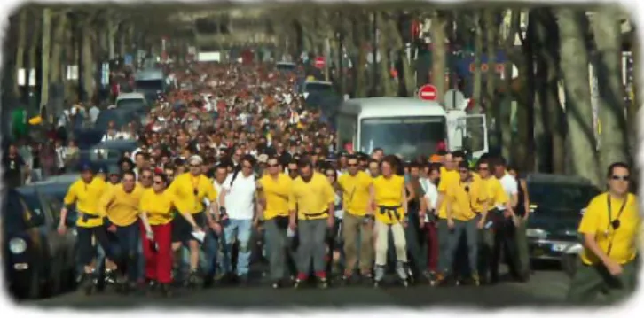
Sunday afternoon in Paris, weather permitting, groups of up to 15,000 people go rollerblading (see Fig. 1). During three hours, rollerbladers travel about 20 miles, covering a large portion of the city. They are guided by staff members and assisted by public safety forces. Participants pause for about 30 minutes after the first half of the course; some of them leave, others join.
Providing participants with ad hoc communication capa- bilities would be highly appreciated. Applications include announcements of itinerary hazards, participant search and gaming, to cite a few. Because of the extreme mobility and intermittent connectivity, the rollerblading tour is a typical scenario of Disruption-Tolerant Network (DTN) [1], [2], [3].
Such networks suffer from frequent connectivity disruptions, which means that there is no guarantee that an end-to-end path exists between a given pair of nodes at a given time.
In disruption-tolerant networks, the mobility of the nodes has a major impact on the performance of communication protocols. It is therefore fundamental to reach a fine-grained understanding of how nodes move. Existing synthetic mobility models (such as the omnipresent random waypoint) are un- able to characterize realistic scenarios. For this reason, many initiatives have provided the research community with real
c Rollers & Coquillages
Fig. 1. Rollerblading tour a Sunday afternoon in Paris.
mobility traces, examples are conferences [3] and university campuses [4]. The analysis of such traces has allowed bet- ter characterization of node mobility and its impact on the dynamics of the network topology. The main observations are based on the concepts of contact and inter-contact times, which generally follow power law distributions.
The RollerNet experiment studies a class of DTNs that follow a pipelined shape. It adopts the classic approach of logging contacts between participants of the roller tour using Bluetooth devices. Our experiment however introduces a new dimension to the data. Besides the contacts between the measurement nodes (iMotes from Intel), we also store contacts with cell phones that have their Bluetooth device on. Although directed, the resulting connectivity graphs exhibit a number of properties that had not previously been observed.
One observation is of particular interest: theaccordion phe- nomenon. The accordion phenomenon, also known as string instability or the slinky effect, can occur in pipelined sets of interconnected systems. Broadly speaking, string stability means that if the initial states of all the interconnected systems are bounded then those states are uniformly bounded for all time. When such stability cannot be guaranteed, a small variation in the state of one system can greatly impact the states of the other systems. This phenomenon has been widely studied in the context of distances between vehicles on a road.
Indeed, if one car slows down slightly, due to the other drivers’
bounded reaction time, it can create a traffic jam among the following cars. The rollerbladers’ movements exhibit a very similar behavior. Indeed, not only do the participants
have a delayed reaction to the others’ movements, but the leaders have to adapt their speed to the slope, red lights, etc.
The resulting accordion phenomenon translates into alternating phases of compression and expansion of the rollerblading crowd. As expected, metrics such as the average node degree, the graph diameter, or the number of connected components vary accordingly.
We focus on the impact of the accordion phenomenon on the delivery delay and traffic overhead. To this end, we evaluate two major routing strategies on our dataset, namely epidemic and spray-and-wait [5]. We study a generalization of the estimation of the epidemic delay proposed by Spyropoulos et al. to the class of d-regular connectivity graphs [6]. This shows that the expected delay in epidemic routing depends on the average degree of the graph. Because of the accordion phenomenon, the average node degree, and thus the expected epidemic delay, fluctuate during the rollerblading tour. The epidemic approach serves as a benchmark for our analysis; it provides both a lower-bound for delay and an upper-bound for overhead.
For the spray-and-wait strategy, both the delay and the overhead are directly related to the number of copies dissem- inated in the spray phase. Indeed, in the absence of any time constraints, spraying a small number of copies may suffice.
However if a target for average delay is set, then one must disseminate a greater number of copies at the cost of a greater overhead. Unfortunately, due to the accordion phenomenon, the delay will vary considerably for a given number of copies.
This results in an often very poor delay-overhead tradeoff.
To counter this problem, we propose DA-SW (Density- Aware Spray-and-Wait), an adaptive variant of the spray- and-wait algorithm that controls the communication overhead while keeping the delay within the expected bounds. The idea behind DA-SW is to exploit the accordion phenomenon and tune the dissemination intensity to respond to the density variation. More specifically, the source sends more copies of a bundle when the topology is sparse and fewer copies when the topology becomes denser. Our results reveal that DA-SW completely counters the accordion phenomenon and dynamically adapts to the current conditions of the network when using a density oracle. Without the oracle, DA-SW still mitigates the accordion phenomenon but not completely due to its delayed reaction to the evolution of the topology.
In short, the contributions of this paper are:
1) New traces.We present a new dataset obtained through real measurements in a rollerblading tour. Because the characteristics of our scenario are inherently different from existing traces, we identify a number of properties that have not yet been observed in other works.
2) Epidemic in d-regular graphs We propose a model for the evaluation of the expected delay of epidemic routing in d-regular connectivity graphs.
3) An adaptive routing. We propose and evaluate a new routing strategy adapted to the mobility observed in our experiment.
The remainder of this paper is organized as follows. In
Section II, we describe in detail the conduct of the experi- ment. Section III analyses data collected during the tour and describes the observed accordion phenomenon. A model of the impact of topology density on the epidemic routing is presented in Section IV, while the presentation of DA-SW, our adaptive routing algorithm, is described in Section V. Related work and previous analysis of real traces are presented in Section VI. Finally, we present our concluding remarks and identify directions for future work in Section VII.
II. THEROLLERNET EXPERIMENT
We capture mobility of participants by deploying contact loggers in the RollerNet experiment [7]. We adopt the tra- ditional approach that consists in deploying contact loggers (Intel iMotes in our case) in a number of participants. Every time a logger discovers a neighboring device, it stores the time and identity of the latter.1 Moreover, as using Bluetooth contact loggers, we also log contacts with other participating Bluetooth devices, like cell phones or PDAs.
Out of the collected data, we characterize the interactions between people over the duration of the rollerblading tour.
Such information is helpful in the design of new forms of ap- plications in the domains of content delivery, location services, and gaming. Such applications should become available in a near future on mobile phones and will take advantage of the phones’ ability to communicate directly with other phones in their vicinity, without passing through the infrastructure.
A. Deployment
The data set we present in this paper has been collected on August 20, 2006. According to organizers and police informa- tion, about 2,500 people participated to the rollerblading tour (few rain showers just before the tour resulted in a number of participants below the average). The total duration of the tour was about three hours, composed of two sessions of 80 minutes, interspersed with a break of 20 minutes.
We deployed contact loggers on 62 volunteers of three types: friends of ours, members of rollerblading associations, and staff operators. In addition to the loggers, we asked other participants to activate Bluetooth on their cell phones. The iMotes also use Bluetooth technology and log periodically (every 15 seconds) the encounters they have with other devices (iMotes or cell phones).2
Fig. 2 presents a schematic view of the deployment orga- nization. During a tour, staff members are organized into six groups. Over the duration of an outing, these groups have an almost static position relative to each other; there are two groups on each side of the crowd, one group at the front, and another one at the end. In order to distribute coverage uniformly among the crowd,25iMotes were entrusted among these six groups. Deploying in this manner, however, does not guarantee that the topology will be connected at all
1The iMotes are small sensor platforms with an ARM7 processor, some on board storage, and Bluetooth capability.
2We detected more than 1,000 cell phones; some were participants of the rollerblading tour, others probably nearby pedestrians.
Fig. 2. Organization of the RollerNet experiment.
times (indeed, we are interested in studying the disruptions that emerge from changing network conditions for devices of limited range). Furthermore, we made sure that among these 25 iMotes, two were given respectively to one staff member always staying at the tail and one staff member always staying at the front. The remaining iMotes have been entrusted as follows: 11 iMotes to friends and 26 iMotes to members of roller skating associations. These latter37devices do not have assigned positions.
B. Sampling issues
All the iMotes ran the same software. As using Bluetooth, two nodes scanning simultaneously are unable to see each other. In order to avoid synchronization of two iMotes around the same cycle clock, we introduced a back-off time of ± 5 seconds around the start time. Due to Bluetooth’s short range, contacts are logged when people get close to each other (typically within ten meters). Nodes performed Bluetooth discovery for 5 seconds every 15 seconds. The number of contacts or the contact times may have been underestimated using such parameters. Other radio technologies, yet not available on mobile phones, such as ZigBee would have been required to sample contacts more precisely.
Because there is a small risk that the Bluetooth inquiry may occasionally miss a contact even though it is present, we made the decision that if a contact is seen at a given inquiryIi, but not at the subsequent inquiry Ii+1, we will still assume that the recorded contact was never broken if we observe it again at the following inquiry Ii+2. Conversely, if a contact is seen at inquiry Ii, but not at inquiries Ii+1 andIi+2, we consider that this contact duration was equivalent to one second.
As this mechanism is implemented directly on the iMotes, and as we record only the beginning and ending of contacts, we drastically reduced memory consumption. Although we could not observe any inter-contact time of less than two inter- vals, this assumption was also made in previous experiments, described in Section VI.
C. Data processing
We also performed a number of post-treatments on the raw traces. First, as no hardware resets have been experienced during the experiment, we had just performed a simple time synchronization using the starting times of each iMote. Sec- ond, as Bluetooth suffers from MAC address corruption, we filtered the dataset and retained only the 1,112 MAC addresses of devices that appeared at least twice. Third, we anonymized
the traces for privacy reasons. And finally, we associated with each iMote a descriptor containing information about the individual carrying the node (whether she or he is a staff member or a regular participant, for instance).
III. ROLLERNET DATA ANALYSIS
In this section, we analyze the dynamics of the rollerblading tour. In order to avoid any biases from the traces obtained during the break phase and from the changes occurred between the rollerblading phases of the tour, we analyze the first 5,000 sec of our data set (before the break). During this period, we recorded 39,305 contacts between the iMotes and 50,193 contacts between the iMotes and 638 external Bluetooth devices (other 413 external devices were detected during the break and the second part of the tour).
We first focus on the accordion phenomenon and how it affects the speed at which information can be disseminated.
For the sake of completeness, we also present results from commonly used analysis which describe pairwise interactions between nodes in contact-oriented data sets.
A. Accordion phenomenon
The accordion phenomenon is due to the alternation of two mobility patterns: pause phases, when skaters wait for safety forces to block the next sequence of crossroads, and rolling phases. To understand the dynamic of network connectivity and characterize accordion effects in the tour, we use the three following metrics:
• Average node degree: We compute the average node degree in a discretized fashion. For each node, the node degree is the number of contacts the node had within an interval of length δ seconds. We then study the evolution of this metric across successive time intervals of δseconds.
• Connected components:As the tour expands and shrinks with time, the topology disconnects. To better understand this dynamic, we measure on graphs obtained every δ seconds, the number of connected components and the size of the giant connected component.
• Average delay: This metric provides, every α seconds, the average delay required for a bundle to travel from any nodeito any nodej given the contact opportunities that we measured.
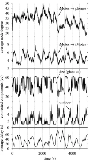
Fig. 3 presents results for δ=15 and α=30. This figure presents five plots (from top to bottom) showing the evolution of: (i) the average node degree for iMote devices considering contacts with external devices, (ii) the average node degree considering only contacts between iMotes, (iii) the size of the giant connected component, (iv) the number of connected components, and (v) the average delay between all pairs of iMotes.
We observe that all these measures followcyclic oscillations being in phase or in opposite-phase with each other. The av- erage node degree is low when participants are rolling (nodes are sparsely distributed in space) and high when the tour shrinks and stops (participants tend to concentrate). It varies
0 20 40 60
0 2000 4000
average delay (s)
time (s) 20
40 60
connected components (cc)
size (giant cc)
0 2 4 6
number 20
25 30 35 40 45 50
average node degree
iMotes → phones
2 4 6
8 iMotes → iMotes
Fig. 3. Average node degree, number and average size of connected components, and average delay over time.
between 17.1 and50.2 when considering contacts only with mobile phones, and between 2.9 and 7.8 when considering contacts between iMotes only. Due to the high number of external devices and the fact that part of them left the tour after t=3,000 sec (due to a little rain shower), oscillations appear in a more fuzzy way when considering external devices.
Furthermore, the number of connected components and the size of the giant connected component oscillate, respectively, in the ranges 1–6 and 19–62. Note that the maximum size of the giant connected component is necessarily 62, as we have only considered iMotes. Although it is intuitive that disconnections occur more frequently when the topology is sparse, it is interesting to underline that we a giant connected component dominates.
Finally, oscillations of the average delay are in opposite- phase with the average node degree, and in phase with the number of connected components. They vary between3.7sec and78.5sec. This result highlights two facts. First, data can be disseminated in average between any two iMotes in32.4 sec;
our initial feeling was that this value would be much higher.
This result is encouraging as it allows a large number of
0 50 100 150 200 250
delay (s)
0 15 30
0 2000 4000
# of relays
time (s)
Fig. 4. Minimum delay and number of relays (when minimizing delay) from tail to head.
applications to operate under reasonable time constraints. Sec- ond, data dissemination is affected by oscillations of network connectivity, being slower when the local density of node is low or when the topology becomes disconnected.
All these synchronized oscillations characterize the so- called accordion phenomenon.
We now look at the effects of the accordion phenomenon on an end-to-end perspective considering the two specific iMotes deployed at the head and tail of the pipeline. Fig. 4 presents the evolution of the minimum delay and the number of relays (when minimizing the delay), required for data to flow from the tail to the head. This figure shows oscillations which are similar and in phase with previous observations. 17.5 relays and52.8sec are required in average. We can also see that the delay roughly varies with the number of relays.
We also evaluate the transition between expansion and shrink phases. Fig. 5 helps understanding the transition phase when passing from pause to moving. This figure presents the average node degree over time, considering contacts with both iMotes and external devices. The head curve shows the results for the first third of the crowd (i.e., the head group) and the tail curve shows the last third of the tour (i.e., the tail group).
Since nodes are not provided with any positioning system, we used the minimum delay required for nodes to send data to the head iMote to estimate their location in the crowd.
We clearly observe that, during the first phase (D, for deceleration), the average degree of head nodes increases before that of the tail nodes. This happens because the tour is slowing down, and the head participants start slowing before the tail ones, increasing their average degree. In the second phase (C, for constant speed), the head nodes are static, which makes their degree constant, while the tail ones continue slowing down. At the end of this second phase, both head and tail have constant (and almost equal) average degree. The third phase (A, for acceleration) represents the evolution of nodes degree when participants start blading again. We clearly see that the head degree decreases quicker than the tail’s one, since the tour’s head shrinks before its tail. The fourth phase (C) represents the whole tour blading, with a constant average degree in both the head and the tail. This phase ends with the beginning of a new cycle, where the head starts slowing and
0 1 2 3 4
average node degree
mobility patterns in function of time
D C A C D
head tail
Fig. 5. Average node degree for head and tail groups of nodes. (A) stands for acceleration period, (C) for constant speed, and (D) for deceleration.
0.1 0.5 1
1 10 100 1000
P(X > x)
average contact (s) RollerNet
Infocom
(a) Contact
0.1 0.3 0.5 0.7 1
10 100 1000 100000
P(X > x)
average inter-contact (s) RollerNet Infocom
(b) Inter-contact Fig. 6. Pairwise average contact and inter-contact time distributions.
so go on. These observations depict the phase transitions faced by the network connectivity due to the accordion effect.
B. Pairwise interactions
We then look at pairwise interactions between nodes con- sidering the commonly used contact-times and inter-contact times. For any pair of nodes i and j, their interactions over time plot times at which they are in contact, called contact times, and times at which they are not in contact, calledinter- contact times. Considering the two statistical processes which generate these two kinds of time intervals helps understanding pairwise interactions of nodes.
We compare results for the RollerNet data set with those of the popular data set introduced by Chaintreau et al. [3] in order to see how much they differ. In this other experiment, iMotes were also used to acquire proximity contacts that occurred between participants of theInfocom 2005research conference.
People intending the conference were asked to carry one of these sensors in their pocket all the time. They collected data from41iMotes over3days. The devices performed Bluetooth inquiry scans every 2 minutes. For each pair of nodes (i, j), we considered, as for RollerNet, that iandj were in contact if either one saw the other. We now use Infocom to refer to this data set.
Fig. 6 presents pairwise average contact and inter-contact times distributions. In both RollerNet and Infocom, pairwise interactions are heterogeneous. We observe that inter-contact times are larger than contact times being in average respec- tively 250 sec and 4 sec for RollerNet and 10,870 sec and
TABLE I
INTER-CONTACT TIME DISTRIBUTION,FITTING RESULTS. Infocom RollerNet Number of pairs tested 737 1394
Exponential 3.3 % 49.6 %
Pareto 5.0 % 6.7 %
Log-normal 99.3 % 99.8 %
None 0.7 % 0.2 %
100 sec for Infocom.3 Finally, the order of magnitude of the two processes is lower in RollerNet than in Infocom.
In order to better characterize pairwise processes, we have tested for whether the distribution of inter-contact times be- tween any two nodes can be modeled either by an exponential, a log-normal, or a Pareto distribution. For this purpose, we use the Cramer-Smirnov-Von-Mises [8] statistical hypothesis test. Recall that such a statistical test can only reject or fail to reject a given hypothesis. So, when the hypothetical distribution is rejected by the test, we are certain that the distribution computed over the data does not match. On the other hand, when the test fails to reject the hypothesis, we only assume that the distribution matches the data to a confidence level 1−α. We used a relatively high level of confidence (α= 0.01) and also visually cross-checked the goodness of fits. For each pair of nodes (i, j)having at least 9 contacts, we have compared the cumulative distribution INij of the N inter-contact times observed and the hypothesized cumulative distribution functions (CDFs). Table I presents, for each data set, the proportion of pairs for which the distribution of inter-contact times fits exponential, Pareto, and log-normal distributions. We also show the proportion of pairs that were rejected for all three hypothetical distributions. Note that, for a given node pair, several distributions may fit the inter-contact distribution.
These inter-contact times are found to follow a log-normal distribution. One notable observation is that log-normal tends to fit better than exponential or Pareto for all three data sets.
The main reason is that the log-normal distribution offers a more versatile model to capture the variability in inter-contact patterns across the different pairs of nodes. We also observe that a larger number of pairs fit an exponential distribution in RollerNet when compared to Infocom.
IV. IMPACT OF DENSITY ON EPIDEMIC ROUTING
Because of the accordion phenomenon, node density and, consequently, node degree vary with time. We have seen that higher degrees offer more favorable conditions for data transfers, improved delivery rates, and shorter delivery times.
In this section, we investigate theoretically the relationship between average degree and delivery delay.
Let us consider a DTN consisting of m nodes. We char- acterize the network density of contact opportunities by the average degree d of the nodes. Every node can only ever
3We recall that contacts observed during only one inquiry in the RollerNet data set are considered to last one second.
meet an average of d other nodes and it will never meet the m − d − 1 remaining ones. We model contact time instants between neighboring nodes as independent Poisson Processes with parameter λ. This implies inter-contact times with exponential distribution, which matches half of the cases in the RollerNet dataset (see Table I). The neighbors of all nodes are chosen with uniform probability and produce a randomd-regular neighborhood graph.
We are interested in computingEepidd , the average delay for transferring a bundle between any two nodes using epidemic routing. For d≥3, the neighborhood graph is always almost surely d-connected, meaning that Eepidd is well defined. A random walk on a grid leads to a connected network (i.e., d = m − 1) with exponentially distributed inter-contact times [6]. In this case, we have that Eepidm−1=λ1Hm−1m−1, where Hn=n
p=11
p is the nthharmonic number. In the RollerNet dataset, degrees vary between 3 and 10 for a total of 62 nodes, so we would like to study the delay of epidemic routing for 3≤d <61(i.e.,3≤d < m−1).
The epidemic delay is computed by gradually coloring all nodes, starting from the source. After each step p, p nodes have received the bundle, and any of them can meet onlys(p) other nodes (their aggregate neighbors). This first encounter takes an average of p s(p)λ1 . At each step, one has the same probabilitym−11 of encountering the target destination. Adding all delay contributions for each of the m−1 steps in the coloring procedure, we obtain the following formula:
Edepid= 1 λ(m−1)
m−1
p=1
m−p
p s(p)· (1) In the random d-regular graph, one can compute s(p) recursively, starting from s(1) = d (the first node has an average of d neighbors). Suppose that the coloring process has reached step p; let us callN(p)the set of colored nodes andS(p)their disjoint neighbors (the neighbors of all nodes in N(p) minus the nodes themselves). The number of elements inN(p)andS(p) are, respectively,pands(p).
Letxbe the node inN(p)which first meets nodey∈S(p).
To generate the two sets at stepp+ 1,yis added toN(p)and removed from S(p). Let us now look at the neighbors of x; x has at least one neighbor inS(p),y. Each of the (m−2) remaining nodes (all the nodes exceptxandy) have the same probability of being any of thex’sd−1remaining neighbors.
Thus, the average number of thosed−1nodes falling inN(p) is (d−1)(p−1)m−2 . Similarly, the average number of nodes falling inS(p)is (d−1)(s(p)−1)
m−2 .
To sum up,S(p+ 1)is obtained fromS(p)by removingy, adding the d−1 neighbors ofy, and removing the neighbors of y which fall in N(p)and in S(p), which translates into:
s(p+ 1) =s(p)−1 +d−1−p−1
nd −s(p)−1 nd , (2) where nd= m−2d−1. Solving the recursive equation above leads to the following formula for s(p),1≤p≤m−1:
0 0.2 0.4 0.6 0.8
10 20 30 40 50 60
expected delay (s)
degree d tail asymptote
head approximation Epidemic
Fig. 7. Delay vs. node degree for epidemic(λ= 1).
s(p) =m−p−
1− 1 nd
p−1
(m−1−d). (3) We can now derive the following result on the behavior of Eepidd for 3≤d≤m−1:
• For d << m, we have Eepidd ≈ K(d)λ , where K(d) =
d−22
∞
p=1 1
p(p+d−22 ). This means that for nodes with a limited number of neighbors, the epidemic delay is not dependent on the size of the network. The formula is obtained from a parabolic approximation of Eq. 2. In this case, the limiting factor is the slow time it takes for the epidemic dissemination to meet all the remaining nodes.
• For d approaching m−1, we obtain Eepidd ≈ 1λ(1d +
Hm−1−1
m−1 ). In this case, the contaminated set may see all the remaining nodes very quickly (after only one step in the approximation) and the limiting factor is the time to see each node one after the other.
Fig. 7 plots the epidemic delay as a function of node degree d for a network of 62 nodes and average intercontact times
1
λ = 1 (normalized). The two extreme behaviors are shown.
For the smallest degrees, the delay drops hyperbolically; for d≥4, we haveK(d)≈ 2d. Ford≥20, the decrease in delay gets smoother and approaches H6161 ≈0.077.
RollerNet falls in the first category with average degrees (3 to 10) much smaller than the number of iMotes (62). The limiting factor for epidemic routing is the degree, whatever the total size of the network. We observe that node density has a direct impact on the delay experienced with epidemic routing.
The formula given in Eq. 1 also shows a sharp hyperbolic drop in the delay with increased node density. One can anticipate that practical routing strategies will behave in a similar way.
Monitoring the density variations, especially for small node degrees, is one of the keys for performing efficient routing in DTNs.
This theoretical result comforts our strategy of designing a routing scheme in which a node dynamically selects the number of bundle copies in function of its connectivity degree.
This is the subject of the following section.
V. MITIGATING THE ACCORDION EFFECT
In this section, we explore the issue of providing a routing scheme that offers to applications packet delivery within
an expected delay bound. For that purpose, we introduce an adaptive strategy that mitigates the accordion effects by controlling the number of copies disseminated in the network in function of the density.
We first study the benefits of such a strategy with O-SW, an Oracle-based version of the Spray-and-Wait routing strategy.
In O-SW, the number of copies is a function of the average density of the network. The results reveal that it is possible to control the average delay while reducing the overhead.
We propose then DA-SW (Density-Aware Spray-and-Wait), a distributed version of O-SW. DA-SW relies on local node degree information to infer the proper number of copies to disseminate.
A. Spray-and-wait routing
To control flooding in DTNs, Spyropoulos et al. propose Spray-and-Wait (SW), a routing strategy in which the source distributes a number of bundle copies to relay nodes that wait to meet the destination [5]. SW faces a natural tradeoff. The number of bundle replicas is related to the probability for at least one of the relay nodes to meet the destination. This has a clear impact on the delay; nevertheless, the more copies are sent, the higher the overhead.
Among the existing methods to disseminate copies, we choose in this work the binary spraying, which is optimal when node movements are independent and identically dis- tributed [5]. In binary spraying, when a node A carrying n copies of a bundle meets nodeB(that does not have any copy of the same bundle), it transfersn/2copies toBand keep the remainingn/2. A node stops sharing its copies either when it meets the destination or when it has one copy remaining. We call SW(n) the binary spray-and-wait algorithm where sources createn copies of the bundles.
B. Oracle-based spray-and-wait
Our first proposal is an oracle-based adaptive algorithm that we call O-SW (Oracle-based Spray-and-Wait). The idea (that will be also considered in the distributed version) is to dynamically determine the number nof copies to be sprayed depending on thecurrent status of the network. The oracle is capable of determining the most adequate number of copies to send depending on some criterion (e.g., to maintain some average end-to-end delay). It serves as a benchmark for our work.
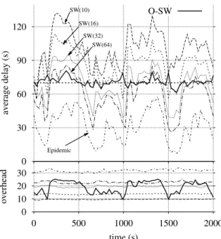
As we are interested in investigating routing, we make simple assumptions regarding lower layers; in particular, we consider infinite bandwidth between nodes, contention free access to the medium, and infinite buffers in the nodes. In order to capture short term variations of network connectivity, we chose to generate bundles every 30 seconds between all pairs of iMotes. We conduct simulations by replaying the first 2000 seconds of the data set introduced in Sec. III. We use the following metrics to evaluate routing performance:
• Bundle delay:the time needed for the first copy to reach destination. Note that since our bundle delivery ratio is
0 10 20 30
0 500 1000 1500 2000
overhead
time (s) 0
30 60 90 120
average delay (s)
SW(10) SW(16)
SW(32) SW(64)
Epidemic
O-SW
Fig. 8. Delay and overhead over time for SW(n) and O-SW.
always 1, our average bundle delay calculations are not biased by discarding the delay of undelivered bundles.
• Overhead:the total number of transmissions needed for bundle delivery. In other words, it quantifies the overhead or the effort spent by the dissemination scheme till a bundle is delivered.
We show in Fig. 8 the results in terms of delay and overhead obtained with O-SW and SW(n). We ran SW(n) with n = {10,16,20,25,32,40,50,64,80,100,128}but, for the sake of presentation, only show in the figure the results for four values ofn. We first observe that, as expected, the higher the number of copies in SW(n), the lower the delay. We can also see that, with O-SW, it is possible to guarantee an average delay by switching from one variant of SW(n) to another (in Fig 8, the target delay is70 sec). In opposition to SW(n) protocols, O- SW leads to an overhead which follows the oscillations of node degree previously seen in Fig. 3. Its overhead varies between 9.8(that of SW(10)) and25.2(that of SW(128)). Using only 11 different values for n, O-SW achieves an average delay of 70.8 sec with a standard deviation of 3.7 sec. This result motivates the use of adaptive routing strategies which control the dissemination effort with regards to node density.
C. Density-Aware Spray-and-Wait
In the previous section, we showed that it is worth using an adaptive algorithm to control the delay/overhead. Nevertheless, obtaining the best case (i.e., with the oracle) is not straightfor- ward. To this end, we propose DA-SW (Density-Aware Spray- and-Wait), a distributed version of O-SW. The goal of DA-SW is to choose, in a dynamic fashion and based only on local information, the right number of copies to achieve constant average delay.
DA-SW relies on the current average node degree in the
0 30 60 90 120 150 180
6 8 10 12
average delay (s)
average node degree
SW(2) SW(4) SW(8) SW(16) SW(32) SW(64) Epidemic
Fig. 9. Average delay for SW(n) and Epidemic vs. average node degree.
roller tour to deriven. This means that the forwarding DA-SW uses an abacus obtained from measurements (for RollerNet, this is done once and reused in future tours, as we expect to have similar behaviors). It is presented in Fig. 9. More specifically, whenever a nodes has a bundle to transmit, it com- putes its current connectivity degree and refers to the abacus to determine the exact number of copies that is expected to lead to some expected delay. In our work, the connectivity degree is the number of neighbors a node has within the latest 30 seconds (we do not address the impact of this measurement window on the performance of our system, and leave it as an interesting topic for future work). The abacus consists in the average delay experienced by a number of SW(n) variants as a function of the average node degree observed when packets were generated. All these curves have been derived from numerical analysis which have been least squares fitted.
In future roller tours, nodes would be pre-charged with the abacus to be used as the reference for DA-SW. Of course, as new experiments are run, the abacus can be enhanced with more data; the system would tend to improve even more.
Fig. 9 also shows values obtained with epidemic routing (lower bound). We can see that the ranking in delay obtained with SW(n) is preserved and that delay decreases faster with node degree when using more and more copies. DA-SW interpolates the right value of n from this abacus using, as input, the observed current average node degree.
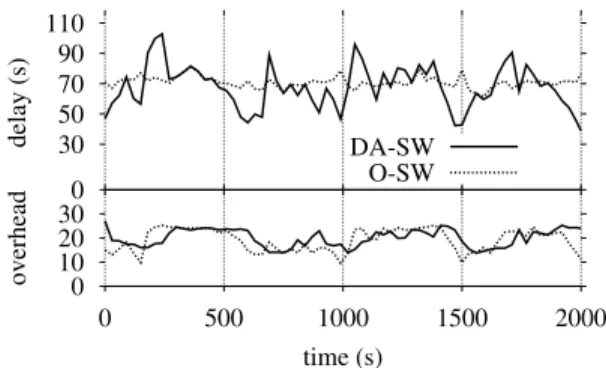
Our goal is to getas close as possible to the results obtained with O-SW. Fig. 10 shows the results for DA-SW when targeting a delay of 70 sec. DA-SW achieves an average delay of 68.1 sec with a standard deviation of 13.9 sec, whereas O-SW achieves an average delay of 70.8 sec with a standard deviation of 3.7 sec. Both DA-SW and O-SW require equivalent overheads, respectively, 19.9 and 19.1 (in number of copies). These results show that DA-SW is able to mitigate the connectivity variations caused by accordion effects to reach a given average delay. However, DA-SW suffers from delay variations compared to O-SW due to a lack of anticipation of aggregation and disaggregation phases (respectively when node density goes up and down). Indeed, when looking at evolutions of overheads for DA-SW and O- SW, we see that they plot similar patterns, but that of DA-SW is behind schedule compared to that of O-SW. This explains
0 10 20 30
0 500 1000 1500 2000
overhead
time (s) 0
30 50 70 90 110
delay (s) DA-SW
O-SW
Fig. 10. Average delay and overhead over time for DA-SW and O-SW.
TABLE II
COMPARISON WITH PREVIOUS IMOTE EXPERIMENTS. Intel Cam-U Infocom Cambridge RollerNet
Duration (days) 3 5 3 10 0.12
δ(mins) 2 2 2 10 0.25
Devices 8 12 41 36 62
Internal contacts 1091 4229 22459 8545 58850
Average #
6.5 6.4 4.6 1.5 280.0
Contacts/pair/day
External devices 92 159 197 3586 1051
External contacts 1173 2507 5791 10469 73661
spikes (up and down) in delay at each phase transition. Good predictors for anticipating changes in mobility patterns would improve performance. We leave this study for future work.
VI. RELATED WORK
There have been a number of efforts to collect mobility data from DTN scenarios in the latest years. The Reality Mining experiment conducted at MIT has captured proximity, location, and activity information from100 subjects over an academic year [9]. Each participant had an application running on her/his mobile phone to record proximity with others through periodic Bluetooth scans and location using information provided by the phone on the cellular network. The UMass DieselNet project investigated the connectivity among40buses in west- ern Massachusetts [2], [10]. In addition to RollerNet, other experiments with iMotes have been conducted by the Haggle project [3], [11], which explores networking possibilities for mobile users using peer-to-peer connectivity between them in addition to existing infrastructures.
For the sake of completeness, we show the similarities and differences between the RollerNet study and the previous ones. We summarize in Table II the main parameters and measurement results from all the experiments, extending the information provided by Chaintreau et al. [3] (Infocom) and Leguay et al. [11] (Cambridge). The experiments Intel and Cam-Uwere performed in corporate and research lab settings, with the participants being researchers and graduate students.
TheInfocomexperiment was conducted during Infocom 2005 and theCambridgeexperiment investigated the feasibility of a city-wide content distribution architecture composed of short range wireless access points. We can see from Table II that the RollerNet dataset is essentially different from existing ones.
In particular, (i) it brings a new dimension to the analysis
by offering a much larger number of contacts, (ii) it leads to enhanced accuracy with a higher frequency of neighbor discovery beacons, (iii) it uses more loggers than previous examples, and (iv) it reveals that nodes see each other much more frequently than in other scenarios.
Additional works have been done to gather data that can be used, after some processing, as DTN-like data. For instance, Henderson et al. [12] have deployed one of the most extensive trace collection efforts to gather information about its Wi-Fi access network at Dartmouth College. These data have been used to characterize the mobility of users [13] or to evaluate DTN routing protocols [14]. Similar Wi-Fi based data have been used to analyze mobility such as that of ETH Z¨urich [15].
Concerning the routing strategy itself, there is a large number of them in the literature. PRoPHET relies on a probabilistic metric calculated using history of encounters and transitivity [16]. Burgess et al. propose the protocol MaxProp [10] which uses meeting probabilities to find paths in association to complementary mechanisms for improving performance in terms of delivery ratio and latency such as buffer management and transmission scheduling. Bin Tariq et al. propose Optimized Waypoints, a distributed algorithm to determine ferry routes to achieve certain properties of end-to- end connectivity, such as delay and message loss among the nodes in the network [17].
Our work definitely contributes to this domain by revealing new findings in a pipelined DTN and bringing a new dataset that is far from being fully analyzed.
VII. CONCLUSION AND OPEN ISSUES
The main contributions of this paper are threefold. First, we present a new dataset obtained through real measurements in a rollerblading tour which falls into the class of pipelined DTNs.
It exhibits a high density of contacts and, more importantly, a clear accordion behavior. To the best of our knowledge, this is the first time an experiment with DTNs reveals such a phenomenon. The RollerNet dataset is available to the research community through the CRAWDAD public archive [18]; it can be used either by the DTN community or by any people interested in the general problem related to the accordion effect. Second, we theoretically motivate that monitoring node density variations, especially for the small node degrees, is a key for performing efficient routing in DTNs, as it has a direct impact in delay on epidemic routing. Finally, we propose DA- SW (Density-Aware Spray-and-Wait), an adaptive variant of the spray-and-wait algorithm that controls the communication overhead while keeping the delay within the expected bounds.
Our results show that we can achieve some expected average delay while limiting the overhead generated in the network.
Future work along these lines includes investigating predic- tors for the average degree so that DA-SW would better antic- ipate changes in mobility patterns. To this end, we intend to perform other experiments of the same kind using other radio technologies such as Wi-Fi or ZigBee (which would improve contact sampling accuracy). Other interesting perspectives are to study and use social communities in the roller tour. Hui
et al. have shown that it is possible to detect social grouping in a decentralized fashion and that it can be used to make efficient forwarding decisions [19]. Further work also remains to be done on resource constraints in terms of node buffers, bandwidth, and energy consumption. Balasubramanian et al.
have shown the routing strategies should fully integrate those parameters when making their forwarding decisions [20].
ACKNOWLEDGMENTS
We thank James Scott and Pan Hui formerly from Intel Research Cambridge for the iMotes that they lent to us and for all the useful discussions. We also thank Timur Friedman and Bruno Dalouche from UPMC Univ Paris 06 for their support and technical help while preparing the deployment. Finally, we are grateful to Philippe Mouli´e and all the staff members from Roller & Coquillages [21]. This work has been partly funded by the French research project ANR CROWD.
REFERENCES
[1] K. Fall, “A delay-tolerant network architecture for challenged internets,”
inProc. ACM SIGCOMM, 2003.
[2] UMassDieselNet, “A Bus-based Disruption Tolerant Network,”
http://prisms.cs.umass.edu/diesel/.
[3] A. Chaintreau, P. Hui, J. Crowcroft, C. Diot, R. Gass, and J. Scott,
“Impact of human mobility on the design of opportunistic forwarding algorithms,” inProc. INFOCOM, 2006.
[4] M. Kim, D. Kotz, and S. Kim, “Extracting a mobility model from real user traces,” inProc. IEEE Infocom, 2006.
[5] T. Spyropoulos, K. Psounis, and C. Raghavendra, “Spray and wait: An efficient routing scheme for intermittently connected mobile networks,”
inProc. WDTN, 2005.
[6] T. Spyropoulos, K. Psounis, and C. S. Raghavendra, “Efficient routing in intermittently connected mobile networks: the single-copy case,”
IEEE/ACM Trans. Netw., vol. 16, no. 1, pp. 63–76, 2008.
[7] “RollerNet: Analysis and use of mobility in rollerblade tours,”
http://www-rp.lip6.fr/rollernet/.
[8] W. Eadie,Statistical Methods in Experimental Physics. Elsevier Science Ltd, 1971.
[9] N. Eagle and A. Pentland, “Reality mining: Sensing complex social systems,”Personal and Ubiquitous Computing, 2005.
[10] J. Burgess, B. Gallagher, D. Jensen, and B. N. Levine, “MaxProp:
Routing for vehicle-based disruption tolerant networking,” inProc. IEEE Infocom, 2006.
[11] J. Leguay, A. Lindgren, J. Scott, T. Friedman, and J. Crowcroft, “Op- portunistic content distribution in an urban setting,” inProc. CHANTS, 2006.
[12] T. Henderson, D. Kotz, and I. Abyzov, “The changing usage of a mature campus-wide wireless network,” inProc. ACM Mobicom, 2004.
[13] M. Kim and D. Kotz, “Classifying the mobility of users and the popularity of access points,” inProc. LoCA, 2005.
[14] J. Leguay, T. Friedman, and V. Conan, “Evaluating mobility pattern space routing for DTNs,” inProc. INFOCOM, 2006.
[15] C. Tuduce and T. Gross, “A mobility model based on wlan traces and its validation,” inProc. IEEE Infocom, 2005.
[16] A. Lindgren, A. Doria, and O. Schelen, “Probabilistic routing in inter- mittently connected networks,” inProc. SAPIR, 2004.
[17] M. M. B. Tariq, M. Ammar, and E. Zegura, “Message ferry route design for sparse ad hoc networks with mobile nodes,” inProc. ACM MobiHoc, 2006.
[18] “CRAWDAD: A community resource for archiving wireless data at dartmouth,” http://crawdad.cs.dartmouth.edu.
[19] P. Hui, J. Crowcroft, and E. Yoneki, “BUBBLE Rap: Social-based forwarding in delay tolerant networks,” inProc. ACM MobiHoc, 2008.
[20] A. Balasubramanian, B. N. Levine, and A. Venkataramani, “DTN Routing as a Resource Allocation Problem,” inProc. ACM Sigcomm, 2007.
[21] “Rollers & coquillages,” http://www.rollers-coquillages.org.