HAL Id: halshs-01961638
https://halshs.archives-ouvertes.fr/halshs-01961638
Submitted on 20 Dec 2018
HAL is a multi-disciplinary open access
archive for the deposit and dissemination of
sci-entific research documents, whether they are
pub-lished or not. The documents may come from
teaching and research institutions in France or
abroad, or from public or private research centers.
L’archive ouverte pluridisciplinaire HAL, est
destinée au dépôt et à la diffusion de documents
scientifiques de niveau recherche, publiés ou non,
émanant des établissements d’enseignement et de
recherche français ou étrangers, des laboratoires
publics ou privés.
Energy Consumption in the French Residential Sector:
How Much do Individual Preferences Matter?
Salomé Bakaloglou, Dorothée Charlier
To cite this version:
Salomé Bakaloglou, Dorothée Charlier. Energy Consumption in the French Residential Sector: How
Much do Individual Preferences Matter?. Energy Journal, International Association for Energy
Eco-nomics, inPress, 40 (3), pp.77-100. �halshs-01961638�
1
Energy Consumption in the French Residential Sector: How Much do Individual Preferences Matter?Salomé BAKALOGLOU1 and Dorothée CHARLIER2
Abstract
The aim of this research is to understand the impact of preference heterogeneity in explaining energy consumption in French homes. Using a discrete-continuous model and the conditional mixed-process estimator (CMP) enable us to address two potential endogeneities in residential energy consumption: energy prices and the choice of home energy characteristics. As a key contribution, we provide evidence that a preference for comfort over saving energy does have significant direct and indirect impacts on energy consumption (through the choice of dwelling), particularly for high-income households. Preferring comfort over economy or one additional degree of heating implies an average energy overconsumption of 10% and 7.8% respectively, up to 18% for high-income households. Our results strengthen the belief that household heterogeneity is an important factor in explaining energy consumption and could have meaningful implications for the design of public policy tools aimed at reducing energy consumption in the residential sector.
Keywords: Residential energy consumption; Household preferences; Discrete-continuous choice method; Conditional mixed-process.
JEL CODES: Q41; D12; C26; C21
1 Salomé BAKALOGLOU, salome.bakaloglou@cstb.fr, Centre Scientifique et Technique du Bâtiment, 84
Avenue Jean Jaurès, 77420 Champs-sur-Marne, Chaire Economie du Climat, 16 Place de la bourse, 75002, Université de Montpellier
2 Dorothée CHARLIER, dorothee.charlier@univ-smb.f, IREGE, Université de Savoie, 74940 Annecy le Vieux
2
1. INTRODUCTION
Reducing the final energy consumption of the European Union has been included in the EU energy strategy for 2030, with the goal of achieving 27% of energy savings compared to the business-as-usual scenario. Among all sectors, decreasing the energy consumption of the buildings sector is one of the most challenging tasks. Despite the fact that the sector has been identified as having the greatest potential for energy savings at the global scale (IEA, 2017), in EU countries the achievement is for the most part subject to the good will and behavior of billions of households living in these buildings (namely, the residential sector)3. Nowadays, observed energy savings are
below the expectations of technical and economic models (Jaffe and Stavins, 1994; Sunikka-Blank and Galvin, 2012; Sorrell and O’Mallay, 2014), which could be a strong indicator of this behavioral bias. In that context, projecting future energy consumption of the sector or changing its trajectory in the expected direction seems complex in the absence of a complete understanding of household behavior.
In terms of policymaking, the task is to implement efficient policies able to stimulate changes at the household level to improve upon international energy consumption targets. Renovation measures and social intervention to encourage more efficient use of energy have been identified as potential solutions for reducing energy consumption in the residential sector (Lopes, et al., 2012). Gaining a better understanding of energy consumption patterns in the housing sector is necessary to implement such solutions in an effective way.
Statistical bottom-up studies conducted by economists have revealed that 40% of energy consumption in the residential sector is determined by technical factors (Belaïd, 2016). A large share of the remainder would be explained by socioeconomic and individual characteristics such as income, age of household members, tenure and energy-related preferences and choices (Belaïd, 2016; Belaïd and Garcia, 2016; Cayla, et al., 2011). Although understanding the determinants of energy consumption has been a recurring theme in economics, distinguishing the effects of individual factors on the final quantity of energy consumed, which would enable characterization of energy behavior and consumption patterns, is still a complex issue. In particular, the topic suffers from limitations due to a lack of appropriate data to control both for socio-economic characteristics, individual preferences and the technical characteristics of dwellings. Consequently, engineering models that almost exclusively use technical building characteristics and engineering calculations as inputs to predict energy consumption are still widely used. However, they reveal limitations in non -including and -modeling the effect of individual heterogeneity and occupant behavior in engineering models (Galvin and Sunikka-Blank, 2014). Combining the benefits of both
3 In 2016, the residential and building sectors represented respectively 25.4 % and 40% of the final energy
3
approaches, namely, integrating both energy-related preferences and theoretical energy performance of housings in research, is an essential step to deepen understanding of the energy consumption spectrum in the residential sector and clarify the role of household behavior.
To advance the academic literature and provide relevant recommendations to policy-makers, additional empirical research is needed to identify individual determinants and their interaction with building characteristics, and to describe energy consumption patterns. Energy savings and energy-intensive behaviors are derived from individual energy use preferences. Analyzing the effect of such preferences is crucial for understanding the importance of household heterogeneity in explaining variability in energy consumption and identifying leverage actions. The issue has generally been neglected in the economics literature (Lopes, et al., 2012), particularly due to the lack of relevant data.
This research aims to partially fill this gap. Our main hypothesis is that individual stated preferences regarding household energy use do have a role in explaining energy consumption in French homes. We used a discrete-continuous model based on McFadden’s pioneering work (1984) to test this assumption, and account for the growing empirical concern related to the interactions between dwellings and household characteristics when modeling energy demand. We assumed that individual energy consumption preferences may be manifested in two ways. We examined whether household comfort preferences and socioeconomic characteristics influence both the features of their home (in this case the energy-efficiency level of the dwelling chosen by the household at the time of purchase or rental), and the amount of final energy they consume. Our research is based on the French PHEBUS4 survey conducted in 2012, which includes complete thermal data, Energy Efficiency Certificates
(energy-efficiency classifications), and socioeconomic characteristics for more than 2000 dwellings, as well as newly available information about household behavior and stated preferences.
This paper thus contributes to the broader literature on the determinants of energy consumption by providing an original analytical framework, thanks to the use of an innovative dataset. A key result is evidence of the existence of several energy consumption patterns in the residential sector that manifest themselves through energy-related preferences and economic characteristics of households. Then, we provide evidence that individual energy use preferences are a significant driver of energy consumption for high-income households, both directly and
4 Performance de l'Habitat, Équipements, Besoins et USages de l'énergie (Phébus)
http://www.statistiques.developpement-durable.gouv.fr/sources-methodes/enquete-nomenclature/1541/0/enquete-performance-lhabitat-equipements-besoins-usages.html
4
indirectly. Our main results show that preferring comfort over economy for two or three types of energy use implies energy overconsumption of 10% on average. If we consider the subpopulation of households belonging to the three highest income deciles, surplus energy consumption from high and medium preferences for comfort lies between 18.1% and 21.8%. For low-income households, we find no significant effect of preferences but a lower energy price elasticity.
Our study differentiates energy consumption patterns by income level, and contributes to the integration of behavioral inputs in modeling exercises, which should be of interest to policymakers. Accordingly, we suggest that policymakers consider low-income and high-income households separately when developing and implementing policies to reduce energy consumption in the residential sector. This is particularly important for reducing potential inequalities and bias. Finally, through our methodology we confirm the necessity of accounting for indirect determinants when assessing the drivers of energy demand in the residential sector.
The paper is organized as follows. Section 2 presents the literature review. Section 3 describes the model. The data and the results are presented in section 4 and 5 respectively. Section 6 concludes with policy recommendations.
2. LITERATURE REVIEW
The final energy consumption of a dwelling is explained by three main determinants: technical building characteristics including the local environment, household characteristics (socioeconomic characteristics, individual preferences, income, etc.), and the price of energy. The literature review also calls attention to the dearth of studies focusing on the share of energy consumption attributed to individual heterogeneity with regard to energy consumption preferences.
Household characteristics
The impact of socio-demographic characteristics on energy consumption has been demonstrated in the literature. Concerning occupancy status, contrary to the theory that posits that tenants are likely to consume more energy than owners (misaligned incentives), empirical research fails to find a consensus on the effect of tenure status on energy consumption (Belaïd, 2016; Charlier, 2015; Jones, et al., 2015; Yohanis, 2012). Family structure and its position in the life cycle, however, does have an impact on energy demand. The number of occupants has a positive impact on energy consumption (Leahy and Lyons, 2010; Vaage, 2000), and there is a cyclical effect based on the
5
age of the reference person: energy consumption is comparatively higher for dwellings whose occupants are between 45 and 65 than for other age classes (Belaïd, 2016; Brounen and Kok, 2011; Brounen, et al., 2013). Regarding income elasticity (see Table I-1 in supplementary materials), the effect is positive in most studies, which is consistent with the “normal good status” of energy consumption: income elasticity often lies between 0.01 and 0.15. This frequent low income elasticity is often attributed to the correlation between income and other characteristics such those of the home (Alberini, et al., 2011) and occupancy status. However, the effect of household income is sometimes more complex. Although low income households use less energy, they have a relatively smaller opportunity to change their appliances and heating and cooling systems. Positive elasticity may mainly involve the purchase of more energy-efficient appliances, which will induce lower energy consumption (Cayla, et al., 2011; Labandeira, et al., 2006; Nesbakken, 2001; Santamouris, et al., 2007). Income elasticity may also depend on income level: in 2013, Meier, et al. (2013) investigated the relationship between household income and expenditures on energy services in the United Kingdom. A key finding of their study was that the income elasticity of electricity and gas demand is contingent on household income. Households with low-income exhibit a rather low-income elasticity of energy demand (about 0.2). Households at the top end of the income distribution exhibit an income elasticity of up to about 0.6. Finally, in the recent work of Hache, et al. (2017), the authors demonstrated with a non-linear approach (CHAID clustering method) that income level and global energy expenditures were intimately related in the French residential sector.
Technical building characteristics and environment
Technical building characteristics and environment can account for more than half of the energy consumption variability in the residential sector. Indeed, much attention has been paid to the impact of the technical properties of housing (insulation, year of construction, building materials, design of the building) on energy consumption. The size effect is positive if we look at its influence on total consumption but is negative if we consider consumption per square meter (“returns to scale effect”). Some estimates indicate that up to 57% of total heating energy consumption can be due to the size effect (Risch et Salmon 2011; Estiri 2015; Baker et Rylatt 2008; Harold, Lyons, et Cullinan 2015). Newer buildings tend to consume less energy, and housing type is an important variable (Nesbakken, 2001; Santin, 2011; Vaage, 2000). Apartments generally consume less than single-family homes because of their smaller heat loss surface (Rehdanz 2007; Vaage 2000; Wyatt 2013). The influence of a dwelling’s construction date on energy consumption (electricity excluded) is not universal, but older buildings generally
6
consume more energy than newer ones (Rehdanz 2007; Risch et Salmon 2011; Vaage 2000). Dwelling insulation (attic or cavity walls or global insulation) reduces energy consumption from -10% to -17% (Brounen, Kok, et Quigley 2012; Hong, Oreszczyn, et Ridley 2006). Finally, local climate also has an impact: in western countries, the longer the heating period is, the more energy a dwelling consumes (Kaza 2010; Belaïd 2017; (Mansur, et al., 2008).
Individual preferences regarding energy use
Individual energy use preferences refer here to the intrinsic disposition of individuals to save energy in their everyday life (Lopes and al. 2012); we do not include individual preferences that are manifested in one-time actions such as the purchase of energy-efficient appliances. Depending on their nature, individual preferences can induce a wide range of everyday behaviors, from energy-saving behavior (energy conservation, restriction) to energy-intensive behavior. The tendency of households to save energy in the residential sector is a multi-dimensional phenomenon resulting from a trade-off between diverging motivations; it is positively linked with environmental awareness and normative concerns or economic motivation and negatively affected by immediate welfare considerations (Lindenberg and Steg, 2007). The work of Hamilton, et al. (2013) demonstrates that energy consumption may differ greatly (by up to three times) among dwellings with similar technical characteristics. Thus, assessing the extent of the effect of individual preferences is a crucial step in better understanding the impact of individual heterogeneity on real energy consumption variability. However, individual preferences have generally been neglected in the economics literature (Lopes, et al., 2012) in particular because of the lack of appropriate data. Assessing the effect of individual energy use preferences on energy consumption variability is complex, and the estimate greatly depends on the indicator used and the scope considered.
Some researchers have approached the issue of preference heterogeneity in energy use by studying the relationship between the effective intensities of energy use for several energy services (e.g. observed energy behaviors such as heating temperature, the running time of appliances, the frequency of use of some energy services, etc.), household and dwelling characteristics, and energy consumption (Belaïd and Garcia, 2016; Santin, 2011; Yun and Steemers, 2011). Santin (2011) found that the number of hours of heating at maximal temperature explains 10.3% of the variability in heating energy consumption. However, in many cases, researchers model energy savings behavior as an end in itself and not as a proxy for individual heterogeneity able to explain energy consumption variability. The major results of these studies show that energy savings actions are context-dependent (Belaïd and
7
Garcia, 2016; Lopes, et al., 2012): living in an energy inefficient dwelling and facing higher energy prices induce more energy-efficient behavior.
Moreover, in the specific case where a household implements energy retrofits to improve the energy efficiency of its housing, the observed savings are sometimes significantly below what can be expected on engineering grounds. Several assumptions can be made to explain this gap. First, measurement errors can occur such as uncertainties in the calculation method used by engineers to assess theoretical energy consumption (Allibe, 2012; Galvin and Sunikka-Blank, 2013; Galvin and Sunikka-Blank, 2014). Second, another conclusion is that there is a strong behavioral bias. Martinaitis, et al. (2015) conducted five different studies to highlight that buildings did not perform as predicted, even when the energy simulation was very accurate. They concluded that human behavior and occupant preferences were important contributors to the gap between the predicted and actual building energy performance. Indeed, a household’s demand for an energy service (or preferences) can evolve over time: this dynamic phenomenon, called direct rebound effect, is well-known in economics literature and research on this topic is widely available. In the residential sector, it is characterized by the increase in thermal comfort after improvement of the energy efficiency of a dwelling. When it occurs, a share of the energy savings potential expected by the implementation of energy retrofits is lost due to behavioral change (Aydin et al., 2017; Sun, 2018). Direct rebound effect for heating could reach 60% (Sorrell, 2009). Finally, the energy savings potential induced by a change in energy related behavior, attitudes or preferences has also been addressed in field experiment studies.
Some small-sample studies on the effect of energy-saving information on energy consumption found that more informative bills and advice about reasonable energy use results in a 10-percent energy savings for electricity (Ouyang et Hokao 2009; Wilhite et Ling 1995). Lopes et al. (Lopes, Antunes, et Martins 2012), found that the savings potential from a change in energy-saving behavior ranges from 1.1% to over 29%.
Energy prices
Price elasticity is always found to be negative, but estimates vary widely from -0.20 to -1.6 (see Table I-1 in supplementary materials section). Energy price elasticities from the literature are listed below. However, it is important to emphasize that the price elasticity of energy demand may depend on the energy considered, the methodology, etc. In their 2017 meta-study Labandeira, et al. (2017) gathered the energy price elasticities results of 428 papers (multi-sector, multi-level, multi-energy sources, multi-country) produced between 1990 and 2016.
8
They showed that the estimates could vary according to the sector, methodology used, level of aggregation of data, nature of the energy source considered, evaluation method, country, etc. For example, their findings provided evidence that micro-level studies tend to find higher price elasticity expressed in absolute values than research based on aggregate models.
Energy price elasticity is also found to be related to income level. For the residential sector in micro-based studies, findings are not unanimous on this issue. For instance, disaggregation of households by expenditure and socioeconomic composition reveals that behavioral response to energy price changes is weaker (stronger) for low-income (top-low-income) households (Schulte and Heindl, 2017). However, Alberini, et al. (2011) found that the price elasticity of electricity demand declines with income, but that the magnitude of this effect is small.
3. DATA AND DESCRIPTIVE STATISTICS 3.1 Data
This research uses data from the PHEBUS survey, a national household energy survey conducted by the Department of Observations and Statistics (SOeS), a subdivision of the French Ministry of Ecology and Sustainable Development. The survey includes 2,040 observations including individual dwelling energy audits performed by the same company in 2012 to study theoretical energy-efficiency measures, real energy consumption (based on energy bills), and reported social, economic, and behavioral data of dwelling occupants. The survey provides cross-sectional annual data (2012) and is representative of the French dwelling stock according to regions, climate zones, dwelling types and building construction dates. The survey was conducted using face-to-face interviews.
Energy performance certificates and building characteristics
Data sets available through this survey are quite innovative as they provide uniform assessments of Energy Performance Certificates (EPC) for each dwelling. These certificates have been produced by a single organization, which reduces any potential subjective bias in performance assessment. In our database, housing energy efficiency is classified into seven energy categories (according to French legislation): A, B, C, D, E, F, G (from the most energy efficient to the least, see Figure II-5 in supplementary materials). In accordance with the literature review, we also introduced the following control variables: housing type, construction period, surface area, the location and climate zone.
9
Real energy consumption
Information on real energy consumption for each dwelling was also available in the PHEBUS survey. For each source of energy consumed at household level, the quantity of energy was assessed from 2012 energy invoices and expressed in kilowatt hours per square meter. Sources of energy used in French dwellings include electricity (31%5), gas (40%), domestic fuel (16%), wood (3.5%), urban heating (5%), etc.
Household characteristics, preferences, and length of tenure
We used income, number of persons, length of occupancy, the number of days of housing vacancy during the heating period, and the number of appliances belonging to each household to control for household characteristics. Information on household stated preferences is available from the PHEBUS survey. Households were asked the following question: “When it comes to indoor heating, do you prefer …?". This question was asked after gathering information about energy-saving behavior.
For each type of end use (heating, hot water, and electricity), a binary variable makes it possible to know whether households favor comfort or energy savings. People can choose to have comfort preferences for one end use and energy saving preferences for another. It is therefore possible to have a scale of preferences. A strong preference for comfort will be measured as a declared preference for each end use, a medium preference as a declared preference for two out of three end uses, and finally a low preference as a single declared preference for comfort. To establish the consistency between stated preferences and energy-saving behavior, we provide Table 1 below.
Table 1: Households’ stated preferences
Preference for...1
Heating end use Comfort Saving energy
Last winter, were you in the habit of regularly lowering the temperature or turning off the heating in the bedrooms …
During daylight 0.28 0.35
At night 0.46 0.52
During the last heating period, when your dwelling was unoccupied, did you …turn off the heat?
Yes 0.36 0.43
When you open the window to ventilate a room, do you turn down or off the heating of the room?
Always 0 .37 0.45
Most of the time 0.43 0.50
Do you limit your heating consumption?
Yes 0.10 0.42
5 The percentage corresponds to the share of households that consume this source of energy as main source of
10
Electricity end use Comfort Saving energy
Number of appliances 16.93 15.49
Hot Water end use Comfort Saving energy
Number of showers (per cu2) 7.57 7.14
Number of baths (per cu) 0.61 0.47
1The null hypothesis of equality of proportions cannot be rejected at the 90% confidence level. All the rest of the
proportions are statistically different at the 90% confidence level or more.
2Index for the number of persons
Note for the reader: This table assesses the consistency between stated behaviors and stated preferences of respondents regarding energy use. Numbers correspond either to proportions of respondents in each category, either to counting numbers (number of baths, of appliances, etc.). For instance, respondents that declared preferring saving energy over comfort are more likely to behave in a more energy saving way regarding the three energy uses: there is a higher share of respondents preferring energy saving over comfort in the category of people that turn down/off the heat when they open the window, these people take a lower number of showers in a week (7.14<7.57) and own a lower number of appliances (15.49 < 16.93).
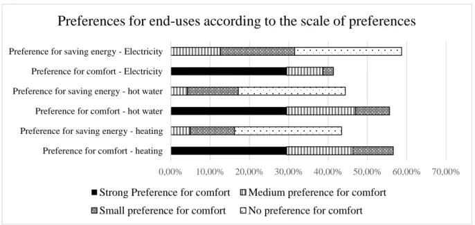
We also compared the preferences for each end use according to our scale (see Figure 1 below). Unsurprisingly, it is not possible to have a strong preference for comfort and a preference for saving energy. For households who have a low preference for comfort, their preference for comfort is mainly for thermal comfort.
Figure 1: Preferences for end uses according to the scale of preferences
Note for the reader: Respondents that declared preferring comfort over energy saving for only one of the three energy uses (small preference for comfort) favour heating use first, then hot water use in second position. Respondents that declared preferring comfort over energy saving for two energy uses (medium preference for comfort) are more likely to favour heating and hot water uses than specific electricity use.
We do not have 100% if we consider each bar separately but if we consider the sum of the answers of the two categories “preference for saving energy” and “preference for comfort” for the same energy use, the result is 100%. Indeed, for each energy use, each respondent had to choose between preferring saving energy or comfort.
0,00% 10,00% 20,00% 30,00% 40,00% 50,00% 60,00% 70,00%
Preference for comfort - heating Preference for saving energy - heating Preference for comfort - hot water Preference for saving energy - hot water Preference for comfort - Electricity Preference for saving energy - Electricity
Preferences for end-uses according to the scale of preferences
Strong Preference for comfort Medium preference for comfort
11
Finally, when people want to save energy, it is mostly for electricity. For example, among households who have medium preferences for comfort, 12.6% want to save electricity compared to only 4.26% for hot water and 4.95% for heating. Moreover, other variables can also be used as a proxy for comfort, for example, the heating temperature (Charlier and Legendre, 2017). SOFRES-ADEME (2009) revealed that an additional one degree Celsius implies an overconsumption of 7.8%.
Energy prices
Unfortunately, the PHEBUS database does not provide energy price information directly. Other information can help determine the energy cost for each household to fill this gap. Indeed, the PHEBUS data set provides information on the type and amount of energy consumed by each dwelling according to each type of fuel, but also on the type of contract (for gas and electricity) and the power required per type of fuel used in kVA (electricity, gas, oil). The power required depends on the type of fuel used for the heating system (i.e. the energy mix) as well as the number of rooms (or the surface area) and the number of appliances. For instance, the power required for electricity is not the same if the heating system is electric or uses another energy source. Thus, it is possible to have different energy power per energy-mix composition and the end use of each type of energy among households. Moreover, for gas and electricity, households can choose the type of contract they want (an energy market supplier or not). Finally, the PHEBUS data set also provides information on the quantity consumed in peak hours and in off-peak hours.
The only information which is not provided is the energy cost itself. To complete the PHEBUS data set, we looked at the PEGASE database (provided by the French Ministry of Energy, see Table II-1 in supplementary materials) to obtain the energy and subscription cost for each type of energy (oil, gas, electricity, and wood) per the amount of power required and the type of contract in 2011 and 2012. Thus, we have information about the price of energy which corresponds to (i) the amount of power required, (ii) the type of fuel, (iii) energy cost in off-peak and peak hours and (iv) the type of contract. We were thus able to fill the gap in the PHEBUS database (see Figure II-1 which sums up the methodology in supplementary materials). Finally, it is possible to calculate a weighted energy cost for each household based on the energy mix and the structure of energy consumption, notably the number of kilowatt hours consumed in off-peak and peak hours. Thus, with a weighted energy cost, we have a specific cost of energy for each household. The equation is as follows:
12
𝑒𝑛𝑒𝑟𝑔𝑦 𝑝𝑟𝑖𝑐𝑒𝑖= ∑ 𝑣𝑜𝑙𝑢𝑚𝑒 𝑖𝑛 𝑘𝑤ℎ𝑖𝑓𝑡×𝑒𝑛𝑒𝑟𝑔𝑦 𝑝𝑟𝑖𝑐𝑒𝑓𝑡 𝑡𝑜𝑡𝑎𝑙 𝑣𝑜𝑙𝑢𝑚𝑒 𝑖𝑛 𝑘𝑤ℎ𝑖 𝑛 𝑖=1 (1)where 𝑓 represents the type of fuel, 𝑖 the household, and 𝑡 the type of rate for a specific energy (electricity or gas).
3.2 Descriptive statistics
The main descriptive statistics of the variables used in the model are summarized in Appendix (Table A1). Based on these observations, we noted several trends in our data. The average income, surface area, occupancy status, etc. seem to be linked in some way with the energy class of each dwelling, which supports the underlying assumption of our model: the potential interaction between home thermal characteristics and household characteristics (Table 2). This is consistent with the contribution of Santamouris, et al. (2007). We also observed interactions between preferences, income level, and consumption (Figure 2, Figure 3, Figure 4, Table II-2, Table II-3 and Table II-4 in supplementary materials). We found that households with high comfort preferences live in dwellings that are statistically more energy efficient. This observation seems consistent with the rebound effect that describes the fact that a cheaper energy cost (due to increased energy efficiency) involves a greater demand for this very same service. Here, the greater demand would mean preferring comfort over saving energy for a specific energy use. Other t-tests confirm the highly significant relationship (p<0.01) between energy consumption, a strong preference for comfort, and income. The overall descriptive statistics argue in favor of the real need to properly control for thermal, economic, and individual characteristics when modeling energy demand in the residential sector.
Table 2: Descriptive statistics by dwelling energy efficiency classification
Energy class* A B C D E F G
Number of observations 5 43 281 564 598 301 248
Average annual disposable income
per household 51068 50099 46097 43970 38632 37877 31201
(22293) (39645) (28396) (25085) (20893) (25569) (18808)
Average number of occupants 3.2 2.9 2.9 2.7 2.5 2.3 2.2
(1.6) (1.2) (1.2) (1.3) (1.2) (1.1) (1.1)
Percentage of individual houses (%) 100 84 79 78 84 81 74
Percentage of renter-occupied
dwellings (%) 0 16 18 19 21 25 35
Mean surface area (m2) 172 151 127.7 118.7. 110 97.5 90.5
(63.3) (92.2) (49.7) (45.7) (47.1) (40.6) (44.0)
Number of years spent in the current dwelling
10.4 10.3 13.1 15.7 18.5 19.5 20.7
(5.8) (9.7) (11.0) (12.8) (15.3) (16.0) (19.9)
Average number of appliances 19.8 22.2 17 16.7 16.6 14.7 12.7
(5.4) (22.5) (11.3) (10.1) (18.4) (11.5) (5.9)
13
*Housing energy classes are defined in supplementary material. Energy Performance Certificates (EPCs) are a rating scheme to summarize the energy efficiency of dwellings. Information about energy efficiency is given as: a numerical value of the energy performance of the dwelling (theoretical energy consumption expressed in kilowatt-hours per square meter) calculated with an engineering model from observed technical characteristics
a ranking into categories of energy performance based on the previous numerical value. Seven categories are defined from G (low energy efficiency) to A (high energy efficiency)
14
4. MODEL
4.1 Theoretical background
For several decades, the framework of conditional demand analysis that employs the two-step discrete-continuous model initiated by Dubin and McFadden (1984) has been used to account for the role of preferences or behavior when modeling energy consumption. More recently, new approaches such as covariance structure analysis or structural equation modeling approach have also been used to integrate indirect determinants of energy consumption. In using these approaches, researchers assume the existence of implicit choices and preferences in terms of home characteristics or energy appliances and their effects on energy consumption. In using discrete-continuous models, researchers also assume that appliance or thermal equipment choices and consumption choice are bound (Dubin and McFadden, 1984; Risch and Salmon, 2017; Vaage, 2000) and use these models to address selectivity biases in data sets with endogenously partitioned observational units (Frondel, et al., 2016). These models are thus often used in the field of energy consumption due to the interactions and endogeneity between independent explanatory variables. Models using the discrete-continuous framework assume that household characteristics could play a twofold role in explaining energy consumption: first, they influence the choice of home characteristics or appliances (indirect effect on energy consumption); second, once the appliances or home characteristics are considered, they also have a direct influence, all things being equal. Kriström (2006) explained that households do not demand energy per se, but demand is combined with other goods such as “capital goods” (housing units, equipment units). Empirical evidence using the discrete-continuous framework has confirmed this assumption: for example, Baker, et al. (1989) applied a two-stage model of energy demand to British expenditure data. Durable good appliances are first modeled, which then determines the energy demand of households. Vaage (2000) and Nesbakken (2001) demonstrated that analyzing energy demand conditionally to appliance or heating system choice is relevant in the residential sector. In the case of France, Stolyarova, et al. (2015) modeled two discrete choices: the choice of end-use combinations by energy source or the choice of heating system by dwelling type.
Recently, researchers have demonstrated further interest in addressing the issue of interactions. Ewing and Rong (2008) showed that higher-income households are more likely to live in big homes that consume more energy. Estiri (2015) called attention to the major interactions between building characteristics and lifecycle and socioeconomic household characteristics and quantified the direct and indirect roles of each in energy consumption with a covariance structure analysis. He reached the conclusion that the main effects of socioeconomic and lifecycle characteristics are observed via building characteristics (expressed with a latent
15
variable that includes surface area, number of rooms, and tenure status). Using a general linear model and a path analysis, Yun and Steemers (2011) investigated the significance of behavioral (the proxy used is frequency of AC use), physical, and socioeconomic characteristics on cooling energy consumption. The findings suggest that such factors exert a significant indirect as well as direct influence on energy use, supporting the necessity of understanding indirect relationships. In the same vein, Belaïd (2017) used a structural equation modeling approach (PLS approach) on French data to elicit the indirect role of household characteristics on building characteristics in order to explain residential energy consumption. His results are consistent with housing consumption theories that socioeconomic household characteristics play an important role in determining the physical attributes of a dwelling. Finally, the importance of accounting for interactions between a dwelling’s physical attributes and household characteristics is also supported by the findings of Santamouris, et al. (2007) in the UK: their work demonstrates that income explains the presence of several dwelling characteristics, including insulation building envelopes and building age.
Based on the existing literature, the main assumption of this research is that individual preference for comfort has a significant positive impact on energy consumption. We assume that the household’s decision is divided into two parts. In the first, the household decides to live in a housing unit according to its theoretical energy performance; then, in the second, it decides how much energy to consume according to its preferences.
To test this assumption, we used a discrete-continuous choice model framework to take into account the assumed interactions between household characteristics and the dwelling’s energy-efficiency level, using a conditional mixed process. The specification of household fuel demand is based on a utility model with R* the stochastic indirect utility function of the households, which we assume to be unobserved. Indirect utility V depends on the price of energy P, income Y, household characteristics (including preferences) Z and building characteristics (including locality) W and is defined conditionally on the choice of energy label classification. Therefore: 𝑅𝑖𝑗∗ = 𝑉𝑖𝑗[𝑃𝑖, 𝑌𝑖, 𝑍𝑖, 𝑊𝑖] + 𝑣𝑖𝑗 (2)
where j=1, ..., J is the index of category, i=1, ...., N that of the individuals, and vij the error term. The Roy's identity
gives us the household's Marshallian demand function for energy: 𝑋𝑖𝑗(𝑃𝑗, 𝑌𝑖, 𝑍𝑖, 𝑊𝑖) =
𝜕𝑉𝑖𝑗(𝑃𝑗,𝑌𝑖,𝑍𝑖,𝑊𝑖)/𝜕𝑃𝑗
𝜕𝑉𝑖𝑗(𝑃𝑗,𝑌𝑖,𝑍𝑖,𝑊𝑖)/𝜕𝑌𝑖 (3)
When simplified, the energy demand function conditional on energy category j by household i can be written as follows:
16
where qij is the quantity of energy consumed by household i in an energy classification j, zij is a vector of household
characteristics (including preferences, income, and mode of occupation), P2012i is the energy price, wij is a vector
of building characteristics (including locality), 𝛾𝑖𝑗 and 𝜈𝑖𝑗 are vectors of the related parameters, and 𝜂𝑖𝑗 the error
term taking into account the influence of unobservable parameters.
4.2 The econometric methodology: a discrete-continuous choice
In our research, an original data set was used to apply this discrete-continuous choice method as we faced two potential problems of endogeneity related to the choice of the dwelling’s thermal performance (energy classifications, see supplementary materials) and endogeneity due to energy prices (proof in supplementary materials). As a choice variable for the discrete choice, we used the theoretical energy performance of the dwelling by energy-efficiency classification. This classification, from an EPC assessment, was chosen as a proxy for the theoretical energy-efficiency level of the dwelling. Thus, we studied which characteristics determine a household’s probability of belonging to an energy-efficient classification level with an ordered probit. Energy classifications have also been introduced in the continuous choice as explanatory variable; this enables us to capture interactions between energy efficiency and households while identifying direct drivers of energy consumption.
Thus, for the discrete choice of the model, we use an ordered probit because energy performance classifications arise sequentially (Cameron and Trivadi, 2010). For individual 𝑖, we specify:
𝑦𝑖∗= 𝑥𝑖′𝛽 + 𝑢𝑖 (5)
with 𝑦∗a latent variable which is an unobserved measure of the dwelling’s energy performance; 𝑥 the regressors.
For low 𝑦∗, energy performance is very high; for 𝑦∗> 𝛼
1 corresponding to the energy classification threshold
A-B to C, energy performance is somewhat lower; for 𝑦∗> 𝛼
2 corresponding to the change from C to D, energy
efficiency is even lower, etc. For an 𝑚-alternative ordered model (here 𝑚 = 6 because of the 6 energy classifications we consider), we define:
17
Pr(𝑦𝑖= 𝑗) = Pr (𝛼𝑗−1< 𝑦𝑖∗≤ 𝛼𝑗)
The regression parameters β and the m-1 threshold parameters 𝛼1, … , 𝛼𝑚−1 are obtained by maximizing the log
likelihood with 𝑝𝑖𝑗 = Pr(𝑦𝑖= 𝑗). Energy classes are also introduced in the second equation and used as regressors
of final energy consumption expressed in kW/m2/year with other explanatory variables. The model captures the
possibility of correlation between unobservable variables in the discrete and continuous stages.
Conditional on the discrete choice, a household decides on the quantity of energy to consume. Therefore, in the continuous choice, the total energy consumption (the logarithm of the energy consumption in kWh/m 2) is
estimated, conditional on the dwelling’s thermal performance (energy-efficiency classification) and a set of explanatory variables (energy price, income, individual preferences, housing characteristics, etc). This is the "energy consumption choice," which we estimate using a least-square model.
On the other hand, , we suspect a risk of endogeneity of the energy price variable in 2012 (P2012i) in the continuous
choice due to simultaneity. Simultaneity arises when at least one of the independent variables is jointly determined by the dependant variable. Here we suspect silmutaneity between the quantity of energy consumed by housings (𝑞𝑖𝑗) and the price of energy (P2012i ). To correct for this potential endogeneity, we implement an instrumental
regression (IV) by introducing as instruments the lag of energy prices (P2011i) that is assumed to not be correlated
with the error term 𝜀𝑖 (cause lagged values are less likely to be influenced by current shocks), and the type of
energy rate for electricity (𝑇𝐴𝑅𝐼𝐹𝐹𝑖), that accounts for the type of contract choosen for electricity and determines
if the energy price is a market or regulated price. According to Robert (2015), estimation strategies using IV are effective when lagged values of the endogenous explanatory variable are used as instruments if the instruments (i) did not appear as explanatory variables in the structural equation and (ii) are well correlated with the simultaneously-determined dependent variable. So, the choice of contract made when the household decides to move in cannot be directly influenced by consumption in the year considered. Finally, some studies which analyze energy consumption using energy prices adopt the same methodology (Risch and Salmon, 2017).
We therefore have:
𝑞𝑖𝑗 = 𝛾𝑖𝑗𝑧𝑖𝑗+ 𝜈𝑖𝑗𝑤𝑖𝑗+ 𝛽𝑖𝑃2012𝑖+ 𝜀𝑖 (6)
with
18
where 𝑞𝑖𝑗 is the final energy per square meter consumed and 𝑧𝑖𝑗 and 𝑤𝑖𝑗 the regressors. We estimate the model
using a double least-squares model, which enables us to correct for the endogeneity issue of energy prices.
Finally, we have a system composed of a three-simultaneous-equations model (5) (6) and (7). The model contains variables which are assumed to explain both choices: the choice of a dwelling with a certain energy-efficiency level and the choice of energy use. However, some exclusion (or selection) variables have also been introduced in each equation: the duration since move-in and detached house for equation 1 (discrete choice) and the number of appliances and number of days of housing vacancy during the heating period for equation 2 (continuous choice).
4.3 The estimation process
In order to estimate our three equations simultaneously, we have used the conditional mixed process (CMP) proposed by Roodman (2011). A CMP framework can be required to jointly estimate three equations with linkages among their error processes. The CMP also allows relationships among their dependent variables. This process fits a large family of multi-equation, multi-level, conditional mixed-process estimators and is particularly useful in the simultaneous equation framework with endogenous variables (as is the case here), or in a seemingly unrelated regressions (SUR)6 configuration, where dependent variables are generated by processes that are
independent but with correlated errors that are not.
Thus, the CMP modeling framework is essentially that of SUR, but in a much broader sense. The individual equations need not be classical regressions with a continuous dependent variable; they also may be estimated by ordered probit. A single invocation of CMP may specify several equations, each of which may use a different estimation technique. Furthermore, CMP allows each equation’s model to vary by observation. The main advantage of the CMP estimator to the SUR estimator is recursivity and full observability that work for a larger class of simultaneous-equation systems. The conditional mixed process is suitable for estimates in which there is simultaneity but where instruments allow for the construction of a recursive set of equations, as in two-stage least square (2SLS). In this case, the CMP is a limited-information maximum likelihood (LIML) estimator. The use of the maximum likelihood approach to estimate the three equations as a system rather than as a two-step estimator implies efficiency gains.
6 See Zellner, A. (1962). An Efficient Method of Estimating Seemingly Unrelated Regressions and Tests for
19
5.RESULTS
5.1 Drivers of energy consumption: discrete-continuous choice model
The results of the two steps are presented in Table 3 below. Complementary results with other measures for preferences and proofs of the quality of estimations are provided in Table A2 in Appendix and in supplementary materials section III-1.
Table 3: Results of the discrete-continuous model
All Samples Decile 1-2-3 Decile 8-9-10
Discrete choice (1) Continuous choice (2) Discrete choice (3) Continuous choice (4) Discrete choice (5) Continuous choice (6)
Energy price in 2012 (log) 0.153** -0.552*** -0.0195 -0.437*** 0.523*** -0.714***
(0.0736) (0.0608) (0.128) (0.111) (0.153) (0.110)
Income (log) -0.112** 0.0921** -0.164 0.0928 0.284* -0.0775
(0.0529) (0.0443) (0.127) (0.111) (0.160) (0.103)
Strong preference for comfort -0.00153 0.102** 0.0974 0.0630 -0.226* 0.181**
(0.0631) (0.0518) (0.114) (0.0992) (0.123) (0.0802)
Medium preference for comfort -0.0609 0.100* 0.103 -0.0127 -0.360*** 0.218**
(0.0677) (0.0558) (0.126) (0.110) (0.131) (0.0896)
Low preference for comfort -0.0532 0.0621 0.0276 0.0848 -0.365*** 0.156*
(0.0675) (0.0555) (0.116) (0.101) (0.139) (0.0947)
No preference for comfort
(reference) - - - -
Number of appliances (log) 0.146*** 0.183*** 0.110**
(0.0324) (0.0671) (0.0515)
Number of days of housing vacancy during heating period (log) -0.0299*** (0.00910) -0.0548*** (0.0172) -0.00775 (0.0152)
Control for individual
characteristics Yes Yes Yes Yes Yes Yes
Control for building
characteristics Yes Yes Yes Yes Yes Yes
Control for locality Yes Yes Yes Yes Yes Yes
Control for building energy class Yes Yes Yes
Control for price endogeneity Yes Yes Yes Yes Yes Yes
N 2,040 2,040 613 613 612 612
Standard errors in parentheses: *** p<0.01, ** p<0.05, * p<0.1
The dependent variable of the discrete choice (ordered probit) is the energy label classification, from G to A-B. The dependent variable for the continuous choice is the energy consumption expressed in kilowatt hour per square meter for the year 2012 (expressed in log).
The thresholds, or cut-off points, reflect the predicted cumulative probabilities at covariate values of zero. They are all significant at p<0.01
Estimates by subgroup of explanatory variables are given in supplementary materials to confirm the robustness of our results. Marginal effects are given in Table III-2 in the supplementary materials section.
Individual characteristics include: number of occupants and duration since last move-in
Building characteristics include: detached or non-detached house, building construction period, surface area
Locality characteristics include: climate zones. In metropolitan France, three main climate zones are considered, they consist of territories with similar temperatures and meteorological conditions (including solar resource). Urban demographic information is also included in locality.
20
5.1.1 Ordered probit (A-B is the reference class)
Results (Table 3) show that household and dwelling characteristics have a significant influence on the propensity to live in an energy-efficient dwelling. Considering the global sample (first column of Table 3), income has a significant negative effect: households with higher income are more likely to live in energy-efficient homes than poor households (see figure III-3 in supplementary materials). This could be linked to the higher price of real estate with better energy efficiency, i.e. “green value” (Hyland, Lyons, et Lyons 2013). This result is also in line with Santamouris, et al. (2007). However, if we consider the subpopulations of the first three income deciles on the one hand (column 3), and of the three last income deciles on the other hand (column 5), income elasticities may differ. We observe that households at the top end of the income distribution are more likely to choose less energy-efficient dwellings; wealthier households generally live in big detached houses which consume more and are less energy-efficient. This result is still valid if we remove the individual preferences for comfort.
Variable energy price has a significant positive effect on the probability of belonging to an energy inefficient dwelling in the global model and the model for deciles 8-9-10, meaning that energy cost can be a driver to choose an energy inefficient dwelling. Energy price could be assumed to reflect the nature of the main energy source of each dwelling, i.e. the heating energy. According to the energy class, the nature of the heating energy differs. Indeed, inefficient dwellings are the dwellings that have the more costing energy sources. For instance, dwellings in class G have fuel and electricity as more frequent main sources of heating energy (see figure III-1 in supplementary materials) and these sources of energy are the more expensive. Thus, a higher energy cost is associated with energy-inefficient dwelling (mostly dwellings heat by electricity and fuel). In average, the cost of fuel is around 0.091 euros per kilowatt-hour, 0.11 for electricity, 0.083 for gas and 0.071 for wood., a higher energy cost is associated with energy-inefficient dwelling.
As the price of energy is higher for the main energy sources of the inefficient dwellings (electricity and fuel), it seems consistent that energy price has a significative positive effect on the fact to belong to an energy inefficient dwelling. Concerning other variables, effects for the global sample are summarized below and are in line with the literature. The age of the reference person has an impact: for the two higher age classes, households are more likely to live in a non-efficient dwelling than those under 44, the effect being higher for households in the last category (over 66 years).
21
Moreover, dwelling occupancy period has a significant link with the energy efficiency of the dwelling. The more recent the move-in date is, the more likely households are to live in efficient dwellings. Two assumptions can be made: the greater availability of energy-efficient dwellings on the current real estate market (new dwellings are more energy efficient because of thermal regulations) and/or greater attention paid by households to residential energy information (for several years, EPC information has been provided to potential renters and buyers). Some environmental characteristics are also correlated with the energy performance of dwellings. Concerning neighborhood, the less isolated the dwelling (in terms of shared walls), the more energy efficient it is likely to be. Urban area types also have an impact; compared to Paris and big cities, dwellings in rural areas are more likely to be energy inefficient; this result is consistent with (Belaïd, 2016). Moreover, energy-efficient dwellings are more likely to be found in cooler climate zones. Finally, size and building type effects are also significant; the bigger the dwelling is, the more energy efficient it is likely to be; living in a bigger house increases the probability of being in an energy-efficient dwelling. A dwelling’s energy efficiency is thus not only determined by household characteristics but also by its environmental and technical characteristics.
Finally, preferences for comfort over economy have a significant effect only in the model applied to households in the three lowest income deciles. Households declaring a preference for comfort for at least one of the three energy uses considered (heating, hot water, or specific electricity) are more likely to live in more energy-efficient dwellings. For a wealthier household, having a strong preference for comfort raises the probability of living in an energy-efficient dwelling (class B) compared to others, from 3.93% to 6.26% (see Table III-2 of marginal effects for order-probit in supplementary materials).
5.1.2 Direct drivers of energy consumption
Energy price elasticity is significant in our three models (columns 2, 4 and 6), ranging from -0.43 to – 0.714; it is consistent with previous findings presented in our literature review. Results show that the magnitude of the price elasticity differs between low and high levels of revenue. It is lower for low-income households (-0.43 in column 4) and higher for high-income households (-0.714 in column 6), meaning that poor households are less responsive to an increase in energy prices. This could be explained by the fact that they are already restricting their energy consumption to their basic requirements; thus, any increase in energy prices does not affect this subsistence consumption. This differentiation in energy price elasticities according to income level is consistent with the work
22
of Nesbakken (1999) and Schulte and Heindl (2017). Income elasticity in the model on the global sample is + 0.09 (column 2), which is consistent with the findings in the literature for countries with similar climate and development characteristics, which range from 0.02 to 0.15. We did not find significant effects of income in the two other models.
Concerning our core assumption about the effect of individual preferences with regard to energy consumption, our model confirms our hypothesis: individual preferences for comfort over economy are highly significant and have a direct positive effect on energy consumption. When the global sample is considered, preferring comfort over economy for two or three energy uses implies energy overconsumption of 10% on average (column 2). If we consider the subpopulation of households belonging to the three highest income deciles (column 6), the effect is significant and even higher: Energy overconsumption from high and medium preferences for comfort lies between 18.1 and 21.8%. Moreover, this result is strengthened by those obtained with the indoor heating temperature (see supplementary materials). A one Celsius degree increase implies an overconsumption of 7.8%. Similar results are presented by SOFRES-ADEME (2009), which showed an overconsumption of 7%.
This result is interesting in terms of public policy development (see section 6). By linking the results of the discrete choice presented above and the descriptive statistics, we can provide a more complete picture of our findings: we demonstrate that richer households are more likely to live in energy-efficient dwellings according to their preferences for comfort among other factors. The effect of individual preferences on energy consumption for these households is positive and higher than that for the global population. Preferences for comfort could induce up to +18% additional energy consumption. This result could be considered to be evidence for the existence of a direct rebound effect even in cross-sectional data. It shows that there is a considerable scope of action for public policies to develop regarding the reduction of energy consumption by behavioral changes for this target population (i.e. wealthier households living in energy-efficient dwellings). Regarding poorer households, we highlight two important facts: they are more likely to live in energy inefficient dwellings where energy is more expensive. Moreover, their response to energy price is low, suggesting that they only address their basic needs regarding energy consumption. The appliance rate of households has also a significant impact on energy consumption. An increase in this rate implies an overconsumption of 14.6%. All these results are consistent with the literature review of Lopes, et al. (2012).
23
Finally, regarding behavioral variables, we see that the duration of absence during the day has, unsurprisingly, a negative significant effect on total energy consumption. The number of appliances is significant and positive in explaining energy consumption. In contrast, the number of days of housing vacancy during heating periods is significant and negative, which is not unexpected. People who work during the day consume less energy.
In terms of dwelling characteristics, energy-efficiency classifications have the expected effects, significant and negative. The more efficient the home is, the less occupants consume energy. This suggests that, in our sample, the EPC measures available in our survey are at least partially representative of the levels of real energy consumption observed. Living in a more energy-efficient dwelling implies a lower effective energy consumption, all things being equal. Finally, climate zone explains both direct and indirect consumption. Living in a cold zone compared to a hot zone has a positive effect on the probability of living in an energy efficient dwelling. Living in cold zone has a positive and significant effect on energy consumption. This result is consistent with the literature, which shows that climate positively influences energy consumption (Kaza 2010; Belaïd 2017; (Mansur, et al., 2008).
6. CONCLUSION AND POLICY IMPLICATIONS
This research provides new evidence of the significant role of individual characteristics in energy consumption. The key result of this research is to provide a preliminary estimate of the magnitude of the effect of heterogeneity in preferences in explaining energy consumption variability. In summary, our research makes the following contributions:
- It confirms the role of common drivers of energy consumption for the French residential sector: energy price, income, age, environmental characteristics, energy efficiency of the dwelling, etc. However, our research also supports the existence of a differentiation of energy price elasticity according to household income level. - It demonstrates that individual preferences for comfort over economy have a significant positive effect on
energy demand for the global population: preferring comfort over economy implies on average a 10% increase in individual energy consumption, all else being equal. We show that this effect is higher in magnitude for high-income households, who are otherwise more likely to live in more energy-efficient dwellings.
- We provide new evidence of the importance of the role of energy label categories when analyzing the drivers of energy consumption. Our methodology applied the well-known discrete-continuous model framework
24
pioneered by McFadden (1984) with a new perspective to account for the complexity of energy consumption. Our modeling of housing choice via the dwelling’s energy-efficiency level (energy classification) is an important contribution. By using a nonlinear methodology to understand the drivers of residential energy demand, our approach, accounting for dwelling/household interactions, is in line with recent work (Estiri 2015, Belaïd 2017). In particular, we provided evidence that basic household and dwelling characteristics (surface area, location, etc.) can determine thermal housing attributes, conditioning final energy consumption.
Based on the findings presented above, in the next paragraph we set out several ways of integrating our research into public policy.
Financial incentives for energy refurbishment
As a result of the discrete choice step of our model, we are in a position to provide a better mapping of the match between household characteristics and the energy characteristics of dwellings. This enables us to formulate policy recommendations aimed at reducing energy consumption through energy efficiency. They are detailed below.
First, we provide evidence that poorer households are more likely to live in energy inefficient dwellings; this means that poorer people live in dwellings that need to be renovated for improved energy efficiency. For these households, the high investment costs of energy retrofits could be a significant barrier to action, which could partly justify the energy efficiency gap observed in the residential sector and well discussed in the academic literature (Gillingham and Palmer 2014).
Second, if we focus on high-income households that are more likely to live in more energy efficient dwellings, attention should be paid to the significant effect of a change in comfort preferences on energy consumption: preferences for comfort could induce up to +18% additional energy consumption. A connection can be made with the well-known “rebound effect” (Gillingham, Rapson, and Wagner 2016) that accompanies better energy performance of a dwelling and leads to a reduced amount of energy savings due to the improvement in comfort resulting from retrofits. In such cases, the household consumes more energy than expected by engineering calculations after the implementation of the energy retrofit. If the rebound effect occurs and is significant, providing financial incentives for energy refurbishment is no longer a cost-effective measure for policymakers. Similarly, Alberini, et al. (2016) provided additional elements relative to the cost-effectiveness of energy retrofits rebates in the residential sector of Maryland (US) and demonstrated that an extreme rebound effect related to electricity heating and cooling consumption was found among incentive takers. His results also suggest that, above
25
a certain level of rebate, the reduction of energy consumption induced by improved energy efficiency no longer exists.
Thus, our research highlights the fact that financial incentives for energy retrofits should be allocated with caution and should target two specific issues: poverty and the cost-effectiveness of public expenditures. In such a context, targeted financial incentives for energy refurbishment should be conditional based on the income level of the household (higher financial incentives for lower income households), on the initial energy-efficiency level of the housing (households living in the least energy efficient dwellings should receive priority) and on the energy-saving potential of the retrofit works to be implemented.
In France, the Live better program funded by the ANAH (National Agency for the improvement of housing) has been part of this approach for several years, offering two levels of income-differentiated incentives to foster energy efficiency in the residential sector. Between 2010 and 2017, about 250,000 dwellings7 were retrofitted with a
minimum theoretical energy efficiency gain set at 25%.
Information and behavioral treatment
Our research highlighted the significant role of a preference for comfort to explain the energy consumption of high-income households. In such a context, the role of behavioral incentives to reduce energy consumption should not be ignored by policy-makers. In line with this recommendation, Zivin and Neidell (2013) used cooling data in the US to argue in favor of the more frequent use of behavioral treatments to reduce energy consumption; they considered these to be just as effective as energy efficiency improvements in bringing about energy savings. Thus, designing information campaigns promoting reasonable energy use and focused on intensive energy consumers unaware of environmental impacts would be an effective complementary tool to reduce energy consumption (Ouyang et Hokao 2009; Wilhite et Ling 1995).
Alternatively, the use of smart meters providing real-time feedback on energy consumption and costs could be a significant way to induce energy-saving behavior (Faruqui, et al., 2010) provided that their widespread deployment can be achieved at a reasonable cost. Numerous studies have demonstrated that improving information about energy consumption can lead to energy efficiency gains (Arrow and Fisher, 1974; Brounen, et
al., 2013; Carroll, et al., 2014; Di Cosmo, et al., 2014; Ehrhardt-Martinez, et al., 2010; Grimes, et al., 2016; Jessoe
7
26
and Rapson, 2014; Matsukawa, 2004; Pon, 2017; Wolak, 2011) Finally, smart metering could also be considered as a tool to fight climate change.
Energy and carbon taxation
Economic tools such as energy taxes or carbon taxation are often considered in the debate as levers for decreasing energy consumption in the short- or long-term. However, some sensitive issues must be carefully addressed regarding our results. We highlighted a lower energy price elasticity for low-income households and a higher cost of energy in less energy efficient dwellings where they are more likely to live: thus, low-income households should be less responsive to economic tools like carbon taxation that increases the energy price and are potentially more affected by its financial consequences. We suggest that policymakers wishing to tax energy or CO2 emissions to be careful not to increase fuel poverty in these households. Specifically, the issue of the redistributive effects of carbon taxation should be carefully addressed by policy makers and academic research. A differentiated energy or carbon tax rate defined according to income level could be envisaged to reduce the redistributive effects mentioned above while taking into account the behavioral patterns observed in high-income households. This could be achieved without extra-cost but could address the issue of social acceptance.
In conclusion, following the results of the research of Hache, et al. (2017), we recommend that policymakers aiming to promote social welfare and achieve effective public policies keep in mind that low-income and high-income households should be considered separately when developing and implementing policies to reduce energy consumption in the residential sector.