HAL Id: hal-02323408
https://hal.archives-ouvertes.fr/hal-02323408
Submitted on 24 Jan 2020
HAL is a multi-disciplinary open access archive for the deposit and dissemination of sci-entific research documents, whether they are pub-lished or not. The documents may come from teaching and research institutions in France or
L’archive ouverte pluridisciplinaire HAL, est destinée au dépôt et à la diffusion de documents scientifiques de niveau recherche, publiés ou non, émanant des établissements d’enseignement et de recherche français ou étrangers, des laboratoires
Large impact of Stokes drift on the fate of surface
floating debris in the South Indian Basin
Delphine Dobler, Thierry Huck, Christophe Maes, Nicolas Grima, Bruno
Blanke, Elodie Martinez, Fabrice Ardhuin
To cite this version:
Delphine Dobler, Thierry Huck, Christophe Maes, Nicolas Grima, Bruno Blanke, et al.. Large impact of Stokes drift on the fate of surface floating debris in the South Indian Basin. Marine Pollution Bulletin, Elsevier, 2019, 148, pp.202-209. �10.1016/j.marpolbul.2019.07.057�. �hal-02323408�
Large impact of Stokes drift on the fate of surface
floating debris in the South Indian Basin
Delphine Doblera,1, Thierry Hucka,∗, Christophe Maesa, Nicolas Grimaa, Bruno Blankea, Elodie Martineza, Fabrice Ardhuina
aUniv Brest, CNRS, IRD, Ifremer, Laboratoire d’Océanographie Physique et Spatiale
(LOPS, UMR 6523), IUEM, Brest, France
Abstract
In the open ocean, floating surface debris such as plastics concentrate in five main accumulation zones centered around 30◦latitude, far from highly turbu-lent areas. Using Lagrangian advection of numerical particles by surface cur-rents from ocean model reanalysis, previous studies have shown long-distance connection from the accumulation zones of the South Indian to the South Pacific oceans. An important physical process affecting surface particles but missing in such analyses is wave-induced Stokes drift. Taking into account surface Stokes drift from a wave model reanalysis radically changes the fate of South Indian particles. The convergence region moves from the east to the west of the basin, so particles leak to the South Atlantic rather than the South Pacific. Stokes drift changes the South Indian sensitive balance be-tween Ekman convergence and turbulent diffusion processes, inducing either westward entrainment in the north of the accumulation zone, or eastward entrainment in the south.
Keywords: Marine debris, Microplastics, Stokes drift, Indian Ocean, Lagrangian analysis, Ocean surface pathways
∗Corresponding author
Email addresses: delphine.dobler@gmail.com (Delphine Dobler),
thierry.huck@univ-brest.fr (Thierry Huck), christophe.maes@ird.fr (Christophe Maes), nicolas.grima@univ-brest.fr (Nicolas Grima), bruno.blanke@univ-brest.fr (Bruno Blanke), elodie.martinez@ird.fr (Elodie Martinez),
fabrice.ardhuin@ifremer.fr (Fabrice Ardhuin)
1. Introduction
Plastics ending at sea are a major issue in our modern societies (Law, 2017). Cózar et al. (2014), van Sebille et al. (2015), Jambeck et al. (2015), among many others, have estimated that tens to hundreds of thousands tonnes of plastics end in the open ocean each year. Floating plastics travel long distances. They tend to accumulate around 30◦ latitude in the five sub-tropical gyres (Martinez et al., 2009; Maximenko et al., 2012) and far from highly turbulent areas (van Sebille et al., 2012). The South Indian Ocean is of particular interest because of the high rate of plastic discharge from the coasts and rivers of the surrounding lands, and the specific dynamics that do not converge around the same longitudes along the basin (Lebreton et al., 2012; van Sebille et al., 2012; Maes et al., 2018).
To simulate the trajectories and accumulation zones of floating debris, Maximenko et al. (2012) and van Sebille et al. (2012) used mean currents com-puted from a surface drifter database (using both those drogued at 15 m and those undrogued) and applied a transfer matrix method. They built the prob-ability matrices of the particles in one grid cell to end up in another grid cell and integrated these matrices over time. Very recently, van der Mheen et al. (2019) used distinct transport matrices constructed from drogued drifter tra-jectories (representing currents at about 15 m depth), and undrogued drifters (representing surface currents), and found a particularly important influence on the southern Indian Ocean garbage patch. With the surface currents transport matrix, the Indian Ocean garbage patch is located to the west of the basin, and is highly dispersive. On the other hand, Maes et al. (2018) and Lebreton et al. (2012) used a method based on Lagrangian advection of nu-merical particles by surface current velocities from an ocean model reanalysis with data assimilation. They also found the five subtropical accumulation zones, but their South Indian accumulation zone is on the eastern side of the basin and leaks eastward towards the South Pacific.
Observations of floating debris are sparse in the Southern Hemisphere (Cózar et al., 2014; Isobe et al., 2019). And although they are compatible with theoretical accumulation in subtropical gyres around 30◦ latitude, they can neither confirm nor refute the zonal location of the South Indian ac-cumulation zone nor the basin to which it most likely leaks. Although the community is building new tools to improve our ocean observation capacity (Maximenko et al., 2019), it will take some time to have accurate datasets.
such a difference in the location of the convergence zone in the South Indian Basin for the different types of simulations. Modelling studies based on the trajectories of Lagrangian particles and using different current products al-low sensitivity experiments particularly adapted to investigate the processes responsible for the displacement of convergence zones.
Ekman convergence is generally believed to be the main physical process responsible for the accumulation of floating debris at 30◦ latitude. The dis-persion by mesoscale turbulence explains why, at 30◦ latitude, accumulation zones tend to be located at the opposite of areas with high Eddy Kinetic Energy (van Sebille et al., 2012). This is particularly true when the basin is broad enough, mainly in the Pacific. Floating debris also feel two other dis-persive forces: the windage, which is the direct wind force felt by the emerged part of a floating object, and the Stokes drift, which results from correlations between velocity and displacement in wind-generated waves. Both windage and Stokes drift are felt by the undrogued drifters used in Maximenko et al. (2012), but are not included in the reanalysis data used in Maes et al. (2018). They could explain the difference observed in the simulations for the South Indian Basin as proposed recently by van der Mheen et al. (2019). We sup-pose that floating plastic debris are less prone to windage than to Stokes drift, as most of them have few or no emerged parts (Beron-Vera et al., 2016). Thus, the impact of windage will not be assessed in this study to adequately separate the different processes. Stokes drift, on the other hand, is of the order of 1% of the wind speed (Rascle et al., 2006; Ardhuin et al., 2009, 2018), with instantaneous values of up to 0.6 m/s in the Antarctic Circumpolar Current and annual averages of 0.2 m/s. Tamura et al. (2012) estimated that the mean annual surface Stokes drift is between 0.02 and 0.10 m/s, and that its horizontal divergence is comparable to Ekman pumping in the North Pacific. In this study, we assess the impact of the surface Stokes drift on the location of South Indian accumulation zone and leak pathways. To properly account for this Stokes drift, a fully coupled ocean-wave model would ideally be required. However, no operational coupled model and corresponding reanalyses were available at the time of this study. Ne-glecting the small-scale fluctuation of Stokes drift introduced by the effect of currents on waves (e.g. Ardhuin et al., 2017) we use a wave model reanaly-sis to estimate Stokes drift, following the method proposed by Isobe et al. (2014). The simple addition of these surface Stokes drift to surface veloci-ties from an ocean model reanalysis will provide an a priori estimate of the impact of Stokes drift, in the same manner as Isobe et al. (2014), Iwasaki
et al. (2017), Fraser et al. (2018), or recently Onink et al. (2019). To under-stand the changes observed in floating debris dynamics, we have also scaled the tracer equation to build a length over which the convergence of Ekman current and eddy dispersion processes are balanced.
This paper describes the impact of Stokes drift on the location of the South Indian accumulation zone and on long-distance leaking pathways, and sheds light on the surface dynamics of the South Indian through the length scale of the balance between convergence and dispersion processes. Section 2 presents the materials and methods, section 3 presents the results of the study in terms of Stokes drift impact and dynamical balance, and section 4 discusses the results and concludes.
2. Materials and methods
2.1. Particle advection by surface currents
As in Maes et al. (2018), we used the Ariane Lagrangian analysis software (Blanke and Raynaud, 1997) to advect numerical particles by surface currents and simulate trajectories of floating debris at the surface. 910,000 particles were introduced at the initial time, homogeneously located with a particle in the center of each ocean surface grid cell of the bipolar C-grid of the ORCA 1/4◦ ocean model. The Ariane software has been configured to prevent these particles from changing vertical levels by assuming that the buoyancy of the floating debris prevents them from sinking.
For the reference scenario, the Ariane software has been fed with the surface current velocities of the CMCC C-GLORS product in its v7 release [dataset] (Storto and Masina, 2016). C-GLORS is a global reanalysis using the NEMO-OPA v3.6 ocean model in the ORCA 1/4◦ configuration and assimilating data such as moorings and remote sensing data, including sea surface height based on altimetry and sea surface temperature. We used the currents from the first layer, which is centered at 0.5 m and is 1-meter thick. The dataset provided to us covers the period from 2005 to 2016 at daily frequency. We first checked that this new version gave the same results as in Maes et al. (2018), which used a previous version.
For the scenario including Stokes drift, we added surface Stokes drift to the C-GLORS surface current velocities. The surface Stokes drift was pro-vided by the IOWAGA dataset which is a reanalysis using the WAVEWATCH III wave model [dataset] (Rascle and Ardhuin, 2013). This method has the advantage of simplicity with immediately available operational products, but
may have two drawbacks: (i) it does not respect the 3D non-divergence cri-terion, and (ii) it assumes that C-GLORS does not include Stokes drift. (i) The ocean models we used enforce volume conservation leading to zero 3D divergence of the velocity field (taking into account the slight freshwater flux at the ocean surface due to evaporation and precipitation). Since we im-pose the particles to remain at the surface, horizontal surface currents are no longer non-divergent, mostly because of their wind-driven Ekman compo-nent (large-scale "geostrophic" ocean currents are mostly non-divergent, in terms of horizontal 2D divergence). Hence the addition of divergent surface Stokes drift does not appear to be a critical issue, as confirmed further by the comparison of the mean divergence of the surface current and of the Stokes drift (Figure 1). (ii) Because C-GLORS assimilates measurement data, and though Stokes drift is not explicitly modelled, some of its physics may be im-plicitly included: however it is very unlikely that the corrections to surface currents are related to the actual Stokes drift. Despite these minor draw-backs, this method will allow us to assess the potential impact of Stokes drift on surface dynamics and particle trajectories. In IOWAGA, the surface Stokes drift is computed from the wave spectrum (which ranges from 0.037 to 0.716 Hz) as follows:
Uss=
Z Z
σ(k) k(k, θ)cosh(2kD)
sinh2(kD) F (k, θ) dk dθ, (1) where k(k, θ) is the wavenumber, σ(k) the wave frequency, F (k, θ) the wave energy spectrum as a function of wavenumber and direction, and D the water depth. In the deep water approximation (kD 1), this simply reads:
Uss =
Z Z
2 σ(k) k(k, θ) F (k, θ) dk dθ. (2)
The surface currents from C-GLORS and the Stokes drift from IOWAGA are not available on the same grid and at the same time frequency. C-GLORS is delivered on an ORCA 1/4◦ bipolar C-grid with averages at daily frequency. The IOWAGA Stokes drift, computed with ECMWF operational analyses and forecasts wind forcing, is delivered on a 1/2◦ regular A-grid at a 3-hour frequency. To add the two components together and conserve an eddy-permitting resolution, the Stokes drift was first averaged daily and then interpolated to the same grid as C-GLORS. This interpolation used the four nearest points weighted by the inverse square distance. At the time
of this study, the IOWAGA dataset forced by ECMWF winds was available continuously for the period 2010 to 2017. Thus, the longest common and continuous period for IOWAGA and C-GLORS products was from 2010 to 2016. To compare the results with previous studies of 29 years of advection (Maes et al., 2018), we made five loops over this 7 year period and analysed the 29th year.
The annual-mean C-GLORS surface currents and IOWAGA surface Stokes drift, and their divergence, are shown in Figure 1. As expected, C-GLORS surface currents are convergent in the main accumulation zones (averaged values over the boxes shown in Figure 1 are between −2 and −3 10−8 s−1, which corresponds to convergence time scales of 1 to 1.5 years) and display the subtropical gyre circulation. In contrast, the IOWAGA surface Stokes drift is divergent in these regions, with averaged values between 0.8 and 1.7 10−8 s−1. This represents up to 50% of the CGLORS surface mean conver-gence and confirms the interest of studying the impact of Stokes drift on particle trajectories.
Figure 1: Annual-mean C-GLORS surface currents (top panel) and IOWAGA surface Stokes drift (bottom panel), represented by arrows, and their divergence (shown by the color scale, convergence in red, divergence in blue). The average was made for the year 2014. The colored boxes are the boundaries of the areas used to compute the mean divergence in the main accumulation zones, as discussed in the text.
2.2. A characteristic length scale of balance
To understand the change in surface dynamics that occurs when Stokes drift is taken into account, we will first consider a scaling diagnosis based on the tracer equation:
∂C
∂t = −∇h(u.C) + ∇h(Kd∇hC), (3) where C = φ ∗ ρ is the particle concentration in number of particles per volume of seawater, φ the number of particles per kilogram of seawater, ρ the density of seawater and Kd the eddy diffusivity coefficient. The first
term on the right-hand side of the equation, −∇h(u.C), is scaled to the
horizontal divergence of the annual-mean velocity field (either by using C-GLORS surface current velocities for the reference scenario, or by adding the C-GLORS surface current velocities with the IOWAGA surface Stokes drift for the Stokes drift scenario). The diffusivity coefficient Kd is scaled
as suggested by Ollitrault and Colin de Verdière (2002) by a characteristic eddy size multiplied by a velocity equivalent to the eddy kinetic energy: Kd≈ Rd1∗
√
2EKE, with Rd1being the first baroclinic Rossby radius [dataset]
(Chelton et al., 1998) and EKE the eddy kinetic energy averaged over one year (as before, either by using C-GLORS surface current velocities for the reference scenario, or by adding the C-GLORS surface current velocities with the IOWAGA surface Stokes drift for the Stokes drift scenario). Scaling the characteristic eddy size by Rd1 stems from Stammer (1997) analyses of the
Topex-Poseidon sea surface heights, where he showed that characteristic eddy sizes were closer to the first baroclinic Rossby radius than to the Rhines scale, especially poleward of 20◦ latitude. This implies that baroclinic instability is the main process of eddy generation on a global scale. The characteristic length Lc over which the convergence balances the diffusion process then
reads for ∇hu < 0: Lc≈ r Kd −∇hu ≈ s Rd1 √ 2EKE −∇hu . (4)
Lc is half the length scale of the "radius of the bell" of Maximenko et al.
(2012) of p4k/|D|, where k is diffusivity and D is divergence. They es-timated this length scale from the e-folding decay scale of particle concen-tration away from the center of the convergence regions and found values
between 700 and 2500 km. But here we have chosen to keep also the infor-mation of divergent points D > 0. If in a region of radius Lc, few divergent
points are encountered, then the particle will tend to stay in this region. To complement this diagnosis, we therefore computed the probability that the particles will encounter divergent points on the length scale characteristic of the balance. For each grid point, we considered the disk of radius Lc/2 and
evaluated the percentage of grid cells where ∇hu > 0. To understand the
zonal entrainment pathways, we zonally averaged this percentage (leak prob-ability) and added the information of the mean zonal current averaged both annually and zonally (leak direction). The zonal means were made between 55◦E and 110◦E in the South Indian Basin.
3. Results
3.1. Impact of the Stokes drift
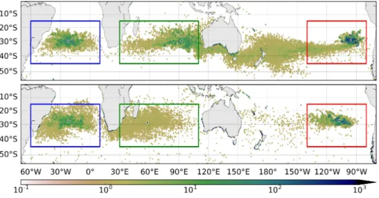
Comparing the concentration of particles after 29 years of advection by ocean model surface currents including or not Stokes drift, we can see that the overall convergence around 30◦ latitude is similar, but that the zonal distribution shows a large difference (Figure 2), as well as the time evolu-tion of the number of particles in each accumulaevolu-tion zone (Figure 3). More specifically, the inclusion of the Stokes drift has a large impact in the South Indian Basin. First, the accumulation zone in the South Indian is sparse and now located on the western side of the Indian basin: the center of mass of the accumulation zone has shifted 32.5◦ to the west. Secondly, 31% of the particles initially located in the South Indian Basin are now found in the accumulation zone of the South Atlantic (compared to 2% without Stokes drift). There are almost no more South Indian particles (0.5%) that end in the South Pacific accumulation zone (compared to 23% without Stokes drift). The time evolution of the number of particles in the South Indian Basin is peculiar compared with the other concentration zones, because it is not monotonic. First, there is an accumulation phase when the South In-dian gains more particles than it loses them. Then there is a second phase when it only loses particles as there are no more particles to gain in the surroundings. The South Indian Basin is leaking, through a specific balance between convergence and dispersion processes that will be discussed more thoroughly in the section about dynamical balance. The time evolution of the particles shows that the South Indian Basin leaks much faster with the Stokes drift, there are almost no more particles in this area at the end of
the simulation, when there were about 80,000 particles without Stokes drift. The South Atlantic accumulation zone still gains particles after 35 years of simulation with Stokes drift, whereas it had reached a maximum after only 7 years of advection without Stokes drift. Finally, the South Pacific accumu-lation zone no longer gains particles with Stokes drift after about 15 years of advection, whereas it still gains particles after 35 years of advection without Stokes drift. This could be partly due to the striking difference in the number of particles stuck to the coast, amounting to 67% after 29 yr of advection with Stokes drift compared to only 20% without Stokes drift. The addition of Stokes drift leads to a net inshore current along several coasts, causing the particles to get stuck in the same place along the coast (the way Ariane software handles "beaching"). The reason for this is twofold: the coastal dynamics of Stokes drift is not well taken into account by the global 1/2◦ IOWAGA product, and the simple addition of Stokes drift implies a strong convergence towards the coast in several regions (as shown in red in Figure 1, bottom panel). Nevertheless, such a process implies difference in the extent of the convergence along the coasts but not in the main pathways and leakage relationships between basins.
In the simulation including Stokes drift, the pathway towards the South Pacific (very clear in Figure 2, top panel) was changed into a pathway towards the South Atlantic, which is more consistent with the results of Maximenko et al. (2012). To illustrate these connections, the trajectories of two parti-cles chosen from the 31% of partiparti-cles that travel from the South Indian to the South Atlantic, and which are representative of the typical trajectories observed for this set, are shown in orange in Figure 4. The corresponding reference particle trajectories (without Stokes drift) are displayed in light blue. Adding Stokes drift, Indian particles tend to flow northeast to 20/15◦S where they are entrained westward by the Indian South Equatorial Current to the east coast of Madagascar. They follow this east coast southward to the Cape Basin and into the South Atlantic. South of the Cape Basin, some particles are taken back northeastward by the South Indian Current or by the Antarctic Circumpolar Current and make one or two additional loops in the Indian Basin before ending up in the South Atlantic. Without Stokes drift, these particles tend to follow the Eastern Gyral Current to the west coast of Australia, then the Leeuwin Current along the west and south coasts of Australia. By adding Stokes drift in our simulation, the main changes are a northwesterly drift in the 35◦-20◦S latitude band and a westward entrain-ment by the Indian South Equatorial Current between 20◦-15◦S, that finally
result in the export of the Indian particles to the South Atlantic Basin.
Figure 2: Lagrangian advection of particles by C-GLORS surface current velocities (top panel) and by the IOWAGA Stokes drift added to C-GLORS surface current velocities (bottom panel). These maps show the particle concentration after 29 years of a simulation that cycled 5 times over the 2010-2016 period for input velocities. The color scale is the concentration of particles per grid cell with a log scale. The colored boxes are boundaries used to display the time evolution of the particles and to compute the percentage of particles from the South Indian Basin ending in the South Atlantic or the South Pacific Basin. The black dots represent the center of mass of the concentration of particles in each colored box.
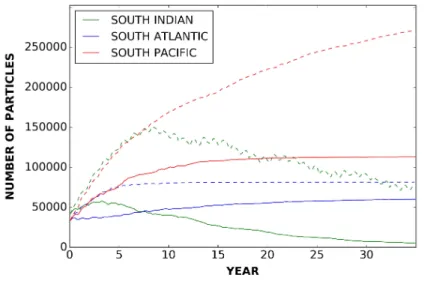
Figure 3: Time evolution of the number of particles in each convergence zone of the South-ern Hemisphere when advected by C-GLORS surface currents only (dashed lines) or by the IOWAGA surface Stokes drift added to C-GLORS surface currents (plain lines). Beached particles (next to a land point) are excluded from the count. It should be noted that a much higher number of particles are blocked along the coast in regions with strong inshore currents when Stokes drift is added (67% totalling 610,000, compared to 20% totalling 182,000 without Stokes drift), hence reducing the total number of particles potentially trapped in convergence regions.
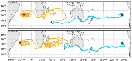
Figure 4: Typical examples of particle trajectories with C-GLORS + surface Stokes drift velocities in orange, and with C-GLORS surface currents only in light blue. The green circles indicate the initial locations and the red squares the final locations after 29 years of advection. The particles were chosen from the 31% (23%) of particles initially located in the South Indian Basin and ending in the South Atlantic Basin (South Pacific) with (without) Stokes drift.
3.2. Comparison with observed drifter trajectories
We would like to compare our results, at least qualitatively, with some of the actual drifter trajectories of the Global Drifter Program (GDP) database [dataset] (NOAA, 2018). This database gathers the locations of more than 23,022 drifters, which are usually drogued around 15 m (Lumpkin et al., 2017). We only considered the locations of drifters when the drogue was lost, which should better represent surface currents (van der Mheen et al., 2019). Undrogued drifters trajectories are unfortunately also subject to windage, but these are the only observations we have with a global coverage, and the most closely related to surface debris. What are the trajectories of undrogued drifters that cross the South Indian Basin and that end in the South Atlantic or in the South Pacific? Using the basin boxes as defined in Figure 2, 1775 drifters cross the South Indian Basin at some point in their lifetimes: 25 of them end in the South Atlantic Basin and 9 in the South Pacific. Because there are so few of them, we have extended the South Atlantic and South Pa-cific boxes to cover the entire width of the basins (Figure 5). Then, 44 drifters end in the South Atlantic, and 49 in the South Pacific. Digging through the detailed trajectories of these drifters, out of the 44 drifters ending in the
South Atlantic, the largest subset, totalling 32 drifters, reaches the Agul-has current from the northeast. Only 6 drifters originated from the eastern part of the Indian Basin and crossed the meridian 60◦E south of 20◦S, and in particular some of them followed the South Equatorial Current approx-imately eastward around 20◦S. 11 drifters originate from the Indian Ocean north of 20◦S, moving southward mostly along the east coast of Madagascar, and along the Tanzania coast. 10 drifters were already in the Mozambique Channel, and 5 in the western part of the basin between 45◦E and 60◦E. The other subset, totalling 12 drifters, enters the Indian Ocean from the southwest before joining the Agulhas current towards the Atlantic: 7 enters the Indian Ocean eastward through the Agulhas retroflection, before moving towards the Atlantic (4 of them were first in the South Atlantic Basin and 3 in the Cape Basin region); 5 come from the Antarctic Circumpolar Channel south of 45◦S and west of 0◦E, and move northeast into the Indian Basin. The 49 drifters ending in the South Pacific all followed very southern pathways: they crossed the South Indian box only through the southeast corner, and were launched south of 45◦S. The other drifters that cross the South Indian box end mainly in the South Indian box, or on the east coast of Africa or on the south coast of Australia (not shown).
In general, the trajectories of drifters are in good agreement with the trajectories of the Lagrangian model including Stokes drift, as shown in Fig-ure 4. It is clear that most of the selected drifters ending in the South Atlantic originate from the South Indian Basin north of 40◦S, whereas most of the selected drifters ending in the South Pacific originate from the South-ern Ocean south of 45◦S (and have entered marginally the South Indian box in its southernmost region). These observations are more consistent with the simulation including Stokes drift, although undrogued drifters are also subject to windage, which is not taken into account in our numerical study, and although there are very few drifters relevant to support robust statistics. Most likely, the life of drifters is too short to see them moving into the South Atlantic or South Pacific (the lifetime is approximately 2 years for a drifter, and an entire loop in the South Indian Basin can take from a few months to a few years), but the South Indian Basin could also leak less rapidly than the simulation suggests.
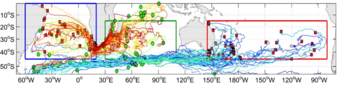
Figure 5: Trajectories of undrogued drifters from the GDP database for drifters that have crossed the South Indian Basin as defined by the green box and that end in the South Atlantic (blue box) or South Pacific (red box). The green circle markers indicate the initial locations, and the red square markers the final locations. The jet colorscale is used to distinguish the trajectories of drifters: The warm (cold) side of the colorscale is used for drifters ending in the South Atlantic (South Pacific).
3.3. Convergence and dispersive dynamical balance
To understand the dynamical mechanisms behind this trajectory change in our simulation, we scaled the tracer equation to estimate the length scale Lcover which convergence and dispersive processes are balanced. This length
scale was computed with one year of C-GLORS surface currents and the re-sulting map is shown in Figure 6. The white color represents the divergent areas, whereas the color scale shows the Lc values computed for the
con-vergent areas. The colorbar has been specially designed to highlight the variations of Lc. The black dots represent the center of mass of the particles
located in each accumulation zone after 29 years of advection with C-GLORS surface currents (like in Figure 2, top panel). The centers of mass in each accumulation zone are in good agreement with the regions containing the least divergent points and a relatively low value of Lc with respect to a given
latitude (because of a strong convergence of the mean currents and low values of Eddy Kinetic Energy). Lc measures the typical horizontal displacement
(in latitude or longitude) of particles subject to the convergence of mean cur-rents and the dispersion by mesoscale turbulence. It could be said that for each location, the least divergent points are encountered in the surrounding region of diameter Lc, the more likely particles will stay around that location.
To assess the impact of including Stokes drift, we compared the Lc values
computed in the reference case (C-GLORS surface currents) with the Lc
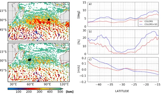
values computed in the case including Stokes drift. The left panel of Figure 7 shows the corresponding maps of Lcfor the South Indian Basin. When Stokes
there seems to be more divergent areas. To quantify these visual impressions, some zonal means have been computed and are shown on the right panel. The graph at the top right shows the corresponding Lc length scale
zonally-averaged over the width of the South Indian Basin (between 50 and 110◦E) and expressed in degrees (Lc[deg] = Lc[km]/Earth_Radius[km] ∗ 180/π).
The figures confirm the overall tendency of higher Lc values with Stokes
drift. The graph in the middle right shows the probability of encountering a divergent point in an area of radius Lc/2, zonally averaged over the width of
the South Indian basin. This can be interpreted as a probability of leakage for South Indian particles. Again, the probability is generally higher with Stokes drift. Focussing on the latitude of the centers of mass 30◦S, this probability is slightly higher just north of 30◦S (up to 24◦S) than just south of it. Finally, the graph at the bottom right shows the zonal currents averaged annually and zonally over the width of the South Indian basin. This is interpreted as a direction of leakage. The current velocities are on average and in absolute value higher with Stokes drift. However, it is also noted that the C-GLORS surface current tends to be slightly eastward or almost zero from 40◦S to 20◦S and that this characteristic changes with Stokes drift: the current is now westward north of about 30◦S. These diagnoses are consistent with the particle advection simulation as shown by the particle trajectories (Figure 4). With C-GLORS currents only, South Indian particles follow the "southern pathway" toward the South Pacific via southern Australia. By adding Stokes drift, South Indian particles follow the "northern pathway" toward the South Atlantic via the Indian South Equatorial current and the Agulhas Current. These results highlight the sensitivity of the South Indian Basin surface dynamics. The values of Lc, the probability of leakage and the
direction of leakage are not very different when considering or not the Stokes drift, but these slight differences altogether cause ultimately a very different fate for floating particles.
Such sensitivity may be related to the specific dynamics of the South-ern Indian Ocean. First, the signature of the eastward South Indian Ocean Countercurrent (Palastanga et al., 2007) is not obvious in terms of surface velocities (Figure 1 and 7c), and is mostly compensated by wind-driven Ek-man velocities. Then, the latitude band extending roughly from 18◦S to 30◦S shows a high level of Eddy Kinetic Energy, associated with prominent long-lived mesoscale structures propagating westward, the South Indian Ocean eddies (Dilmahamod et al., 2018), that could also contribute to the west-ward advection of particles.
Figure 6: Characteristic length Lc (in km) over which the convergence and diffusion
processes are balanced for the C-GLORS surface currents. The data were smoothed in space over distances of 1◦. The white color corresponds to positive divergence values. The black dots correspond to the centers of mass of the accumulation in each convergence zone for year 29 of the corresponding simulation of particle advection by the Ariane software (as defined in Figure 2).
Figure 7: Probability and direction of leakage in the South Indian. Left panels: Character-istic length scale Lc (in km) over which convergence and diffusion processes are balanced
for the C-GLORS (top) and C-GLORS + Stokes drift (bottom) surface currents in the South Indian Basin. Right panels: zonal means over the South Indian Basin for a) the characteristic length Lc of the balance between convergence and diffusion; b) the
proba-bility of encountering a divergent point on a disk with a radius Lc/2; c) the zonal velocity
averaged zonally and annually.
4. Discussion and conclusion
Using drifter buoy data, Maximenko et al. (2012) and van Sebille et al. (2012) have shown that floating debris tend to accumulate mainly in the subtropics. Their prediction of the location of accumulation zones is fairly consistent with the few available observations (Cózar et al., 2014; van Sebille et al., 2015). In particular, their South Indian accumulation zone lies on the western side of the basin and leaks towards the South Atlantic. Using surface currents from an ocean-model reanalysis, Maes et al. (2018) have also found five accumulation zones in the subtropics but their dynamics of the accumulation zone in the South Indian is very different: the accumulation zone is located on the eastern side of the basin and particles leak towards the South Pacific. To understand which physical processes are responsible for this change of behaviour in the South Indian, we investigated the
influ-ence of Stokes drift which impacts undrogued drifters and surface floating debris. The main idea is to reconcile the different models and datasets used in previous studies, according to the physical processes taken into account.
The inclusion of Stokes drift has indeed a major effect on the fate of par-ticles in the South Indian Ocean. The parpar-ticles initially in the Indian Basin no longer travel eastward to the South Pacific but westward to the South Atlantic: they are entrained westward by the Indian South Equatorial Cur-rent at 20◦S, they reach and follow southward the east coast of Madagascar, follow the Agulhas Current, and end in the South Atlantic. We rationalized this change in dynamics by constructing a characteristic length scale Lcover
which the convergence and the diffusion processes are balanced. The maps of this length scale correspond fairly well to the center of mass of the ac-cumulation zones. The account of Stokes drift has increased both Lc and
the probability of encountering divergent points within a radius of scale Lc.
It also favored a slightly higher probability of leakage north of 30◦S than south, associated with stronger westward average current in this area. These diagnoses are consistent with the results of particle advection simulations. Overall, it mainly shows that particles dynamics in the South Indian Basin is very sensitive and that particles from the South Indian could either stay in the South Indian Basin or take the southeast pathway to the South Pacific, or take the northwest pathway towards the South Atlantic.
In our simulation, the Stokes drift changed the balance in the South Indian Basin from an entrainment of floating particles to the east to an entrainment to the west. More generally, the inclusion of Stokes drift causes particles to change their trajectory or to be more entrained on the northwest pathway if they are already following it. However, Stokes drift influences only the upper few meters at the ocean surface (Clarke and Van Gorder, 2018, for instance), and the vertical distribution of microplastics over the global ocean is largely unknown (Kukulka et al., 2012; Reisser et al., 2015; Song et al., 2018). Consequently a significant fraction of the microplastics in the subsurface layer are probably not influenced by Stokes drift and follow more generally the surface currents (the wind-driven Ekman component decreases with depth on a scale of about 10 m, much larger than Stokes drift). It is thus useful to keep in mind the different scenarios of particle advection by surface currents with and without Stokes drift.
Our results, which use only particle trajectories, are consistent with the recent and thorough analyses by van der Mheen et al. (2019), which used different transport matrices based on surface and 15 m deep dynamics to
explain the particular sensitivity of the Southern Indian convergence region. Both studies confirm that more realistic surface currents (including Stokes drift) lead to a convergence region of the Southern Indian located west of the basin, and leaking towards the South Atlantic Basin. Our main addition to their results is that Stokes drift alone is sufficient to move the Southern Indian convergence region westward, whereas their study associates Stokes drift with a 1% wind speed windage. According to their study, changes in mean surface currents are sufficient to explain this displacement. In our simulations, the Indian convergence region does not appear as dispersive as in their results, and this is still obvious after 30 years of integration (maybe because the leakage to the Atlantic is weaker in our simulations) – in any case, this appears to be a second-order issue for microplastics, since a large and regular supply of debris from the Asian coasts of the Indian Basin continuously feeds this convergence region against dispersion and leakage to the South Atlantic. However, a comparison with their figures shows that the variability of currents (as opposed to their use of a single "mean" transport matrix) is important to support "super"-convergence routes to other ocean basins (Maes et al., 2018). This variability is also important to allow the connection between the North Indian Basin (where large quantities of plastics enter the ocean) and the South Indian Basin, apparently a significant difference with their simulations (not shown here).
Although our study provides a good a priori knowledge of the impact of Stokes drift, it suffers from several approximations that should be addressed. The first approximation stems from the method chosen to include the Stokes drift itself. This additive method, based on the available reanalysis datasets, does not meet the 3D non-divergence criterion and assumes that no Stokes drift is present in the surface currents of the C-GLORS reanalysis, which can-not be fully verified because of the assimilation of surface data. The second approximation stems from the interpolation and daily average of Stokes drift on the C-GLORS space-time grid. The signal loss due to these smoothings should be quantified more precisely. As a first step, we ran an additional Ar-iane experiment where surface currents including Stokes drift were provided every 3-hours instead of every day: they were computed from the daily C-GLORS surface currents and 3-hour surface Stokes drift, as provided by the IOWAGA reanalysis, and simply interpolated to the C-GLORS spatial grid as described earlier. The results were surprisingly similar to those presented above for convergence regions and pathways. The only difference we have seen is a significant decrease in the number of particles that get stuck at the
coast (57% after 29 yr of advection with the 3-hourly currents, instead of 67% with the daily currents), which could result from the stronger variability at high frequencies.
On the same topic, Maes et al. (2018) pointed out that eddy mesoscale variability is essential for constructing exit routes from the South Indian Basin. The grid used for the C-GLORS reanalysis is at 1/4◦ and is therefore only eddy permitting, not eddy resolving. The impact of current fields at a finer resolution, in such a sensitive region, is probably not negligible and should also be quantified (for instance Wang et al., 2015, about the Agulhas leakage and transport through the South Atlantic). In our simulation, we inseminated particles only at a given initial time and homogeneously over the whole ocean, but the sources of floating plastic debris are not homogeneously distributed. In order to make a consistent comparison with observation maps of floating debris, we should now adapt our particle input scenario to a more realistic scenario, both in space and time. The sensitivity of the trajectories of surface floating debris in the Indian Basin is particularly important to understand and quantify, as a large fraction of the world’s plastic waste is released in this area, with significant input from Asian rivers (Lebreton et al., 2018) and a very large population living on its coasts.
Acknowledgements
This work was supported by the French National Research Agency (ANR) under the "Programme d’Investissements d’Avenir" ISblue (ANR-17-EURE-0015) and by LabexMER (ANR-10-LABX-19). We are grateful to Andrea Cipollone (CMCC) for providing the CGLORS surface current dataset, Mick-ael Accensi for his help with the IOWAGA dataset and Xavier Couvelard for interactions on coupled ocean-wave models.
Ardhuin, F., Aksenov, Y., Benetazzo, A., Bertino, L., Brandt, P., Caubet, E., Chapron, B., Collard, F., Cravatte, S., Dias, F., Dibarboure, G., Gaultier, L., Johannessen, J., Korosov, A., Manucharyan, G., Menemen-lis, D., Menendez, M., Monnier, G., Mouche, A., Nouguier, F., Nurser, G., Rampal, P., Reniers, A., Rodriguez, E., Stopa, J., Tison, C., Tissier, M., Ubelmann, C., van Sebille, E., Vialard, J., Xie, J., 2018. Measuring cur-rents, ice drift, and waves from space: the sea surface kinematics multiscale monitoring (SKIM) concept. Ocean Sci. 14, 337–354.
Ardhuin, F., Marié, L., Rascle, N., Forget, P., Roland, A., 2009. Observa-tion and estimaObserva-tion of Lagrangian, Stokes, and Eulerian currents induced by wind and waves at the sea surface. Journal of Physical Oceanography 39 (11), 2820–2838.
Ardhuin, F., Rascle, N., Chapron, B., Gula, J., Molemaker, J., Gille, S. T., Menemenlis, D., Rocha, C., 2017. Small scale currents have large effects on wind wave heights. J. Geophys. Res. 122 (C6), 4500–4517.
Beron-Vera, F. J., Olascoaga, M. J., Lumpkin, R., 2016. Inertia-induced accumulation of flotsam in the subtropical gyres. Geophysical Research Letters 43 (23), 12,228–12,233.
Blanke, B., Raynaud, S., 1997. Kinematics of the Pacific Equatorial Under-current: an Eulerian and Lagrangian approach from GCM results. Journal of Physical Oceanography 27 (6), 1038–1053.
URL http://www.univ-brest.fr/lpo/ariane/
Chelton, D. B., deSzoeke, R. A., Schlax, M. G., El Naggar, K., Siwertz, N., 1998. Geographical variability of the first baroclinic Rossby radius of deformation. Journal of Physical Oceanography 28 (3), 433–460.
URL http://www-po.coas.oregonstate.edu/research/po/research/rossby_radius/ Clarke, A. J., Van Gorder, S., 2018. The relationship of near-surface flow,
Stokes drift and the wind stress. Journal of Geophysical Research: Oceans 123 (7), 4680–4692.
Cózar, A., Echevarría, F., González-Gordillo, J. I., Irigoien, X., Úbeda, B., Hernández-León, S., Palma, Á. T., Navarro, S., García-de Lomas, J., Ruiz, A., Fernández-de Puelles, M. L., Duarte, C. M., 2014. Plastic debris in the
open ocean. Proceedings of the National Academy of Sciences 111 (28), 10239–10244.
Dilmahamod, A. F., Aguiar-Gonz alez, B., Penven, P., Reason, C. J. C., De Ruijter, W. P. M., Malan, N., Hermes, J. C., 2018. SIDDIES corridor: A major east-west pathway of long-lived surface and subsurface eddies crossing the subtropical south indian ocean. Journal of Geophysical Re-search: Oceans 123, 5406–5425.
Fraser, C., Morrison, A., Hogg, A., Macaya, E., Van Sebille, E., Ryan, P. e. a., 2018. Antarctica’s ecological isolation will be broken by storm-driven dispersal and warming. Nature: Climate Change 8, 704–708.
Isobe, A., Iwasaki, S., Uchida, K., Tokai, T., 2019. Abundance of non-conservative microplastics in the upper ocean from 1957 to 2066. Nature Communications.
Isobe, A., Kubo, K., Tamura, Y., Kako, S., Nakashima, E., Fujii, N., 2014. Selective transport of microplastics and mesoplastics by drifting in coastal waters. Mar. Pollut. Bull. 89 (1-2), 324–330.
Iwasaki, S., Isobe, A., Kako, S., Uchida, K., Tokai, T., 2017. Fate of mi-croplastics and mesoplastics carried by surface currents and wind waves: A numerical model approach in the Sea of Japan. Mar. Pollut. Bull. 121 (1-2), 85–96.
Jambeck, J. R., Geyer, R., Wilcox, C., Siegler, T. R., Perryman, M., An-drady, A., Narayan, R., Law, K. L., 2015. Plastic waste inputs from land into the ocean. Science 347 (6223), 768–771.
Kukulka, T., Proskurowski, G., Morét-Ferguson, S., Meyer, D. W., Law, K. L., 2012. The effect of wind mixing on the vertical distribution of buoy-ant plastic debris. Geophysical Research Letters 39 (L07601).
Law, K. L., 2017. Plastics in the marine environment. Annual Review of Marine Science 9, 205–229.
Lebreton, L., Slat, B., Ferrari, F., Sainte-Rose, B., Aitken, J., Marthouse, R., Hajbane, S., Cunsolo, S., Schwarz, A., Levivier, A., Noble, K., Debel-jak, P., Maral, H., Schoeneich-Argent, R., Brambini, R., Reisser, J., 2018.
Evidence that the Great Pacific Garbage Patch is rapidly accumulating plastic. Scientific Reports 8 (1), 2045–2322.
Lebreton, L.-M., Greer, S., Borrero, J., 2012. Numerical modelling of floating debris in the world’s oceans. Mar. Pollut. Bull. 64 (3), 653 – 661.
Lumpkin, R., Ozgokmen, T., Centurioni, L., 2017. Advances in the applica-tion of surface drifters. Ann. Rev. Mar. Sci. 9, 59–81.
Maes, C., Grima, N., Blanke, B., Martinez, E., Paviet-Salomon, T., Huck, T., 2018. A Surface “Superconvergence” Pathway Connecting the South Indian Ocean to the Subtropical South Pacific Gyre. Geophysical Research Letters 45 (4), 1915–1922.
Martinez, E., Maamaatuaiahutapu, K., Taillandier, V., 2009. Floating ma-rine debris surface drift: Convergence and accumulation toward the South Pacific subtropical gyre. Mar. Pollut. Bull. 58 (9), 1347–1355.
Maximenko, N., Hafner, J., Niiler, P., 2012. Pathways of marine debris de-rived from trajectories of Lagrangian drifters. Mar. Pollut. Bull. 65 (1), 51 – 62.
Maximenko, N., et al., 2019. Towards the integrated marine debris observing system. Front. Mar. Sci.
NOAA, 2018. Global drifter program.
URL http://www.aoml.noaa.gov/phod/gdp/index.php
Ollitrault, M., Colin de Verdière, A., 2002. SOFAR floats reveal midlati-tude intermediate North Atlantic general circulation. Part II: an Eulerian statistical view. Journal of Physical Oceanography 32 (7), 2034–2053. Onink, V., Wichmann, D., Delandmeter, P., van Sebille, E., 2019. The role
of Ekman currents, geostrophy and Stokes drift in the accumulation of floating microplastics. Journal of Geophysical Research: Oceans 124. Palastanga, V., P., van Leeuwen, J., Schouten, M. W., de Ruijter, W. P. M.,
2007. Flow structure and variability in the subtropical Indian Ocean: In-stability of the South Indian Ocean countercurrent. Journal of Geophysical Research 112, C01001.
Rascle, N., Ardhuin, F., 2013. A global wave parameter database for geo-physical applications. Part 2: Model validation with improved source term parameterization. Ocean Modell. 70 (x), 174–188.
URL https://wwwz.ifremer.fr/iowaga/
Rascle, N., Ardhuin, F., Terray, E. A., 2006. Drift and mixing under the ocean surface. a coherent one-dimensional description with application to unstratified conditions. J. Geophys. Res. 111, C03016.
Reisser, J., Slat, B., Noble, K., du Plessis, K., Epp, M., Proietti, M., de Son-neville, J., Becker, T., Pattiaratchi, C., 2015. The vertical distribution of buoyant plastics at sea: an observational study in the North Atlantic Gyre. Biogeosciences 12, 1249–1256.
Song, Y. K., Hong, S. H., Eo, S., Jang, M., Han, G. M., Isobe, A., Shim, W. J., 2018. Horizontal and Vertical Distribution of Microplastics in Ko-rean Coastal Waters. Environ. Sci. Technol. 52 (21), 12188–12197.
Stammer, D., 1997. Global characteristics of ocean variability estimated from regional TOPEX/POSEIDON altimeter measurements. Journal of Physi-cal Oceanography 27 (8), 1743–1769.
Storto, A., Masina, S., 2016. C-GLORSv5: an improved multipurpose global ocean eddy-permitting physical reanalysis. Earth System Science Data 8 (2), 679–696.
URL http://c-glors.cmcc.it/index/index.html
Tamura, H., Miyazawa, Y., Oey, L.-Y., 2012. The Stokes drift and wave induced-mass flux in the North Pacific. Journal of Geophysical Research 117 (C08021).
van der Mheen, M., Pattiaratchi, C., van Sebille, E., 2019. Role of indian ocean dynamics on accumulation of buoyant debris. Journal of Geophysical Research: Oceans in press.
van Sebille, E., England, M. H., Froyland, G., 2012. Origin, dynamics and evolution of ocean garbage patches from observed surface drifters. Envi-ronmental Research Letters 7 (4), 044040.
van Sebille, E., Wilcox, C., Lebreton, L., Maximenko, N., Hardesty, B. D., van Franeker, J. A., Eriksen, M., Siegel, D., Galgani, F., Law, K. L., 2015.
A global inventory of small floating plastic debris. Environmental Research Letters 10 (12), 124006.
Wang, Y., Olascoaga, M. J., Beron-Vera, F. J., 2015. Coherent water trans-port across the south atlantic. Geophys. Res. Let. 42, 4072–4079.