HAL Id: hal-03155400
https://hal.archives-ouvertes.fr/hal-03155400
Submitted on 28 May 2021HAL is a multi-disciplinary open access
archive for the deposit and dissemination of sci-entific research documents, whether they are pub-lished or not. The documents may come from teaching and research institutions in France or abroad, or from public or private research centers.
L’archive ouverte pluridisciplinaire HAL, est destinée au dépôt et à la diffusion de documents scientifiques de niveau recherche, publiés ou non, émanant des établissements d’enseignement et de recherche français ou étrangers, des laboratoires publics ou privés.
Sensitivity Analysis of the Interfrequency Correlation of
Synthetic Ground Motions to Pseudodynamic Source
Models
Seok Goo Song, Mathieu Causse, Jeff Bayless
To cite this version:
Seok Goo Song, Mathieu Causse, Jeff Bayless. Sensitivity Analysis of the Interfrequency Correlation of Synthetic Ground Motions to Pseudodynamic Source Models. Seismological Research Letters, Seismological Society of America, 2020, 92 (1), pp 301-313. �10.1785/0220200181�. �hal-03155400�
Seismological Research Letters
Sensitivity Analysis of the Inter-frequency Correlation of Synthetic Ground Motions to
Pseudo-dynamic Source Models
--Manuscript Draft--Manuscript Number: SRL-D-20-00181R2
Full Title: Sensitivity Analysis of the Inter-frequency Correlation of Synthetic Ground Motions to Pseudo-dynamic Source Models
Article Type: Article - Regular Section Corresponding Author: Seok Goo Song, Ph.D.
Korea Institute of Geoscience and Mineral Resources Daejeon, KOREA, REPUBLIC OF
Corresponding Author Secondary Information:
Corresponding Author's Institution: Korea Institute of Geoscience and Mineral Resources Corresponding Author's Secondary
Institution:
First Author: Seok Goo Song, Ph.D. First Author Secondary Information:
Order of Authors: Seok Goo Song, Ph.D. Mathieu Causse Jeff Bayless Order of Authors Secondary Information:
Manuscript Region of Origin: KOREA, REPUBLIC OF
Abstract: Given the deficiency of recorded strong ground motion data, it is important to
understand the effects of earthquake rupture processes on near-source ground motion characteristics and to develop physics-based ground motion simulation methods for advanced seismic hazard assessments. Recently, the inter-frequency correlation of ground motions has become an important element of ground motion predictions. We investigate the effect of pseudo-dynamic source models on the inter-frequency correlation of ground motions by simulating a number of ground motion waveforms for the 1994 Northridge, California, earthquake, using the Southern California Earthquake Center (SCEC) BroadBand Platform (BBP). We find that the cross-correlation between earthquake source parameters in pseudo-dynamic source models significantly affects the inter-frequency correlation of ground motions in the frequency around 0.5 Hz while its effect is not visible in the other frequency ranges. Our understanding of the effects of earthquake sources on the characteristics of near-source ground motions,
particularly the inter-frequency correlation, may help to develop advanced physics-based ground motion simulation methods for advanced seismic hazard and risk assessments.
Suggested Reviewers: Arben Pitarka LLNL
pitarka1@llnl.gov Expertise in the field Hiroe Miyake ERI, Japan
hiroe@eri.u-tokyo.ac.jp Expertise in the field Fabrice Cotton GFZ, Germany
Robert Graves USGS
rwgraves22@gmail.com Expertise in the field Kim Olsen
SDSU
kbolsen@mail.sdsu.edu Expertise in the field Opposed Reviewers:
Sensitivity Analysis of the Inter-frequency Correlation of Synthetic Ground Motions to 1
Pseudo-dynamic Source Models 2
3
Seok Goo Song1, Mathieu Causse2, and Jeff Bayless3 4
5
1Earthquake Research Center, Korea Institute of Geoscience and Mineral Resources (KIGAM),
6
Daejeon, Republic of Korea 7
2Univ. Grenoble Alpes, Univ. Savoie Mont Blanc, CNRS, IRD, IFSTTAR, Univ. Gustave Eiffel,
8
ISTerre, Grenoble, France 9
3AECOM, Los Angeles, USA
10
11
CORRESPONDING AUTHOR 12
Seok Goo Song 13
Address: 124 Gwahang-no, Yuseong-gu, Daejeon 34132, Republic of Korea 14 Tel: +82-(0)42-868-3296 15 Email: sgsong@kigam.re.kr 16 17 18
Manuscript (clean copy) Click here to
ABSTRACT 19
Given the deficiency of recorded strong ground motion data, it is important to understand the 20
effects of earthquake rupture processes on near-source ground motion characteristics and to 21
develop physics-based ground motion simulation methods for advanced seismic hazard 22
assessments. Recently, the inter-frequency correlation of ground motions has become an 23
important element of ground motion predictions. We investigate the effect of pseudo-dynamic 24
source models on the inter-frequency correlation of ground motions by simulating a number of 25
ground motion waveforms for the 1994 Northridge, California, earthquake, using the Southern 26
California Earthquake Center (SCEC) BroadBand Platform (BBP). We find that the cross-27
correlation between earthquake source parameters in pseudo-dynamic source models 28
significantly affects the inter-frequency correlation of ground motions in the frequency around 29
0.5 Hz while its effect is not visible in the other frequency ranges. Our understanding of the 30
effects of earthquake sources on the characteristics of near-source ground motions, particularly 31
the inter-frequency correlation, may help to develop advanced physics-based ground motion 32
simulation methods for advanced seismic hazard and risk assessments. 33
INTRODUCTION 35
Ground motion prediction is an important element of the assessment of seismic hazards. 36
In particular, for advanced seismic hazard assessment endeavors, it is important to understand 37
the near-source ground motion characteristics of large events. Empirical ground motion 38
prediction equations (GMPEs) have been used extensively to predict ground motion intensity 39
measures such as the peak ground acceleration (PGA) and pseudo-spectral acceleration (PSA) 40
(e.g., Abrahamson et al., 2008). However, although ground motions have been recorded 41
worldwide, the quantity of recorded strong ground motions is insufficient to investigate the near-42
source characteristics, i.e., the intensity and variability of ground motions near earthquake fault 43
rupture (Chiou et al., 2008). Recently, physics-based ground motion simulation approaches, 44
including both dynamic and pseudo-dynamic earthquake rupture models, have become more 45
popular for evaluating the near-source ground motion characteristics such as the effect of rupture 46
directivity and fault complexity (e.g., roughness), given the availability of advanced numerical 47
modeling schemes and rapidly growing high-performance computing capabilities (Olsen et al., 48
2009; Graves et al., 2011; Shi and Day, 2013). 49
GMPEs predict both the mean and the standard deviation of ground motion intensity 50
measures such as PGA and PSA, given a set of explanatory seismological parameters 51
(magnitude, distance, site conditions, etc.). Recently, several research groups pioneered a method 52
to investigate the inter-frequency (or inter-period) correlation characteristics of ground motions 53
by analyzing recorded ground motion data (Baker and Cornell, 2006; Baker and Jayaram, 2008; 54
Stafford, 2017; Bayless and Abrahamson, 2019a). The inter-frequency correlation characterizes 55
the relative width (in the frequency domain) of the extrema in a ground motion spectrum. The 56
widths of the peaks and troughs in ground motion spectra are significant in assessments 57
involving simulated ground motions because the variability in dynamic response analyses can be 58
underestimated if simulated ground motions have an excessively low correlation (Bayless and 59
Abrahamson, 2018). 60
It would be meaningful to investigate whether physics-based ground motion simulation 61
models can produce the inter-frequency correlation of ground motions, consistent with empirical 62
correlation models, obtained by analyzing recorded ground motion data. There have been several 63
attempts to understand how well the physics-based ground motion simulation models reproduce 64
the mean and the standard deviation of ground motion intensity measures, produced by empirical 65
GMPEs (Cotton et al., 2013; Causse and Song, 2015; Imtiaz et al., 2015; Vyas et al., 2016; 66
Crempien and Archuleta, 2017; Moschetti et al., 2017; Wirth et al., 2017). Recently, Wang et al. 67
(2019) implemented an inter-frequency correlation model obtained by analyzing recorded ground 68
motion data in their physics-based broadband ground motion simulation platform. In other 69
words, they developed a post-processing method for their synthetic ground motion waveforms to 70
mimic the inter-frequency correlation structure observed in the empirical model. However, we 71
think that this study is a first attempt to understand the direct link between physics-based ground 72
motion simulation models and the inter-frequency correlation of ground motions. 73
In this study, we adopted the pseudo-dynamic source modeling method, proposed by 74
Song et al. (2014) and Song (2016), for physics-based ground motion simulations, which is 75
implemented at the SCEC BBP. Pseudo-dynamic source modeling approaches maintain the 76
computational efficiency of kinematic source modeling methods but emulate the essential 77
physics of earthquake rupture dynamics by statistically analyzing a number of dynamic rupture 78
models (Guatteri et al., 2004; Graves and Pitarka, 2010; Schmedes et al., 2013; Song et al., 79
2014). Fayjaloun et al. (2019) and Park et al. (2020) successfully investigated the effect of the 80
pseudo-dynamic source models, developed by Song et al. (2014) and Song (2016), on the mean 81
and the standard deviation of ground motions. In this study, we investigated the effect of the 82
pseudo-dynamic source models on the inter-frequency correlation of ground motions. We first 83
performed a series of ground motion simulations for the 1994 Northridge, California, earthquake, 84
using various sets of pseudo-dynamic source models. Then we investigated the sensitivity of the 85
inter-frequency correlation of the simulated ground motions to those pseudo-dynamic source 86
models. 87
88
GROUND MOTION SIMULATION 89
For this research, we adopted the broadband platform (BBP) developed by the Southern 90
California Earthquake Center (SCEC) for synthetic ground motion simulations (see Data and 91
Resources). Multiple research groups, including both earthquake scientists and engineers, have 92
been involved in the SCEC BBP project (Goulet et al., 2015; Maechling et al., 2015). The BBP 93
has been thoroughly validated against both actual ground motions recorded during past 94
earthquakes and empirical GMPEs (Dreger et al., 2015; Goulet et al., 2015). The latest version of 95
the BBP is released regularly; here, we used V. 16.5, which was released in May 2016. Multiple 96
modeling schemes are provided in the platform; we chose the Song method, which uses pseudo-97
dynamic source models, based on the 1-point and 2-point statistics of earthquake source 98
parameters (Song et al., 2014; Song, 2016). The Song method adopts the Graves and Pitarka 99
(GP) method (Graves and Pitarka, 2010) for the simulation of high-frequency (> 1 Hz) ground 100
motions as well as the low-frequency (< 1 Hz) seismic wave propagation. The GP method adopts 101
the Green’s function computation method developed by Zhu and Rivera (2002), given a 1-102
dimensional velocity model. In this study, we primarily aimed to investigate the inter-frequency 103
correlation of ground motions in the low-frequency range, i.e., between 0.1 and 1.0 Hz. Thus, we 104
expect that the inter-frequency correlation is mainly affected by the pseudo-dynamic source 105
models, implemented in ground motion simulations. 106
The SCEC BBP performed two types of validation (Goulet et al., 2015). The first 107
validation (Part A) was against ground motion data recorded during past earthquakes in North 108
America and Japan. The second (Part B) was against empirical GMPEs. Among the Part A 109
validation events, we chose the 1994 Northridge, California, earthquake for our study. Detailed 110
information about the fault plane geometry of the event is given in Table 1 and Figure 1. The 111
Northridge event occurred in a highly populated area and produced well-recorded ground 112
motions, as shown in Figure 1. For the details of the event simulation, we followed the procedure 113
established by the SCEC BBP group (Goulet et al., 2015). 114
Given the fault geometry defined in Table 1, we prepared three sets of pseudo-dynamic 115
rupture models for our sensitivity test, as summarized in Table 2. Furthermore, we employed the 116
input source statistics models proposed by Song (2016), which are also summarized in Table 3. 117
The basic set (Test Set I) in Table 2 is composed of two groups of pseudo-dynamic source 118
models. One group contains correlated source models, while the other contains uncorrelated 119
source models. The core element in the pseudo-dynamic source models proposed by Song et al. 120
(2014) is the cross-correlation structure coupling the earthquake source parameters, such as the 121
slip, rupture velocity, and peak slip velocity. For the group of uncorrelated source models, we 122
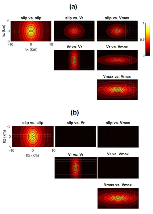
simulated the pseudo-dynamic source models without a cross-correlation structure, as visualized 123
in Figure 2. Several studies have been performed to understand the effects of the cross-124
correlation structure on near-source ground motions, particularly the mean and the standard 125
deviation of ground motion intensity measures such as the peak ground velocity (PGV) and PGA 126
(Fayjaloun et al., 2019; Park et al., 2020). 127
However, whereas the authors of these studies perturbed each cross-correlation 128
component individually for their sensitivity analysis, we focused on two cases, i.e., full cross-129
correlation (correlated) and no cross-correlation (uncorrelated) between the earthquake source 130
parameters, as shown in Figure 2. For Test Set I in Table 2, we simulated 100 pseudo-dynamic 131
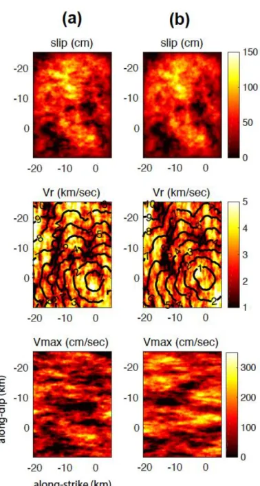
source models, i.e., 50 correlated and 50 uncorrelated source models. Figure 3 shows the first 132
three source models among the 50 models in the group of correlated source models, while Figure 133
4 shows the first three for the group of uncorrelated source models. In the correlated source 134
models, the source parameters (such as the slip, rupture velocity, and peak slip velocity) are 135
coupled together according to the cross-correlation structure in Figure 2a. Since the pseudo-136
dynamic source models are obtained by stochastic modeling, based on the covariance matrix 137
constructed by the input source statistics models (Song et al., 2014), each source model exhibits 138
unique randomness; nevertheless, we can observe correlations between the source parameters in 139
Figure 3. In contrast, the distributions of the source parameters within the models depicted in 140
Figure 4 display heterogeneity, controlled by the diagonal elements of Figure 2b, but no coupling 141
between the source parameters is expected. 142
We also prepared two additional sets of pseudo-dynamic source models, i.e., Test Sets II 143
and III in Table 2, for our sensitivity analysis. In Test Set II, we randomly perturbed the 144
hypocenter of each source model. In the Part A validation, following Goulet et al. (2015), the 145
hypocenter was fixed since the validation was performed for real past events. We adopted the 146
same strategy for Test Set I. However, the hypocenter location may significantly affect the near-147
source ground motion characteristics. Therefore, since we aimed to investigate the sensitivity of 148
ground motions to various dynamic source models rather than to validate our pseudo-149
dynamic source models against recorded ground motion data, we decided to test random 150
hypocenter models in Test Set II as well. 151
In Test Set III, we perturbed the stress drop by increasing or decreasing the rupture 152
dimension while holding the seismic moment constant. Since the stress drop directly affects the 153
corner frequency and hence the shape of the Fourier amplitude spectrum (e.g., Causse and Song, 154
2015), the stress drop may also affect the inter-frequency correlation characteristics of ground 155
motions.The static stress drop is proportional to the ratio of the mean slip to the characteristic 156
rupture dimension (𝐿̃), as given in the equation below (Kanamori and Anderson, 1975): 157
∆𝜏 ≈𝜇𝑠𝑙𝑖𝑝
𝐿̃ . (1)
158
Models with larger stress drops were obtained by decreasing both the rupture length and the 159
width by 30%, while models with smaller stress drops were obtained by increasing both the 160
rupture length and the width by 30%. The input source statistics for each model are presented in 161
Table 3. Figures 5 and 6 show one example each of the simulated pseudo-dynamic source 162
models with larger and smaller stress drops, respectively.In Test Set III, there are 300 pseudo-163
dynamic source models, i.e., 150 correlated and 150 uncorrelated models, as indicated in Table 164
2. The 150 correlated source models contain 50 models with larger stress drops and 50 with 165
smaller stress drops in addition to the 50 correlated source models from Test Set I. 166
Using the SCEC BBP (V. 16.5), we simulated three-component ground motion 167
waveforms at the 133 stations illustrated in Figure 1 for each pseudo-dynamic source model. The 168
Song method adopts a hybrid approach, i.e., pseudo-dynamic low-frequency (< 1 Hz; Song, 169
2016) and stochastic high-frequency (> 1 Hz; Graves and Pitarka, 2010) modeling schemes. For 170
a systematic sensitivity analysis of the simulated ground motions with a single representative 171
metric for the ground motion intensity measures, we adopted the effective amplitude spectrum 172
(EAS), computed with two horizontal-component ground motions as (Bayless and Abrahamson, 173
2018) 174
𝐸𝐴𝑆(𝑓) = √12[𝐹𝐴𝑆𝐻𝐶1(𝑓)2+ 𝐹𝐴𝑆𝐻𝐶2(𝑓)2], (2)
175
where 𝐹𝐴𝑆𝐻𝐶1 and 𝐹𝐴𝑆𝐻𝐶2 are the Fourier amplitude spectra of the two orthogonal horizontal
176
components of the three-component waveforms and 𝑓 is the frequency in Hz. The EAS is 177
independent of the orientation of the instrument. Using the average power of the two horizontal 178
components (Eq. 2) leads to an amplitude spectrum that is compatible with the application of 179
random vibration theory to convert the Fourier spectra into response spectra. The EAS is 180
smoothed using the log10-scale smoothing window of Konno and Ohmachi (1998) with the
181
smoothing parameters described by Kottke et al. (2018). 182
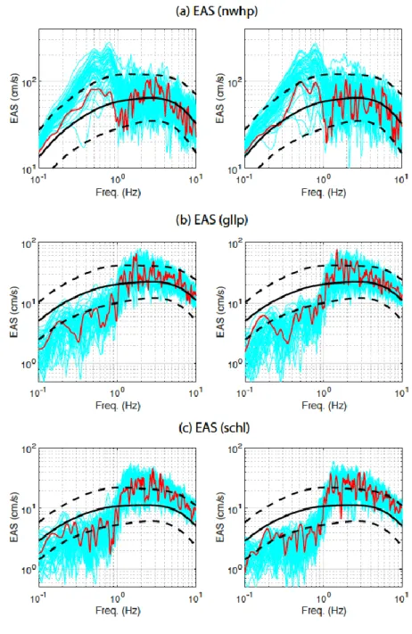
Figure 7 shows examples of the EASs for the three selected stations plotted in red in 183
Figure 1. For the near-source station (nwhp, Rrup = 5.4 km), the low- and high-frequency EASs
184
do not differ considerably, but for the other two stations (gllp, Rrup = 21.5 km; schl, Rrup = 40.4
185
km), the two frequency bands, i.e., the low-frequency (< 1 Hz) and high-frequency (> 1 Hz) 186
bands, show distinctive EAS patterns. Since we used the abovementioned hybrid approach, the 187
low- and high-frequency ground motions may not behave consistently for all rupture scenarios 188
and station locations. This issue may need to be investigated further for all hybrid ground motion 189
simulation methods offered by the SCEC BBP. In this study, we aimed predominantly to analyze 190
low-frequency (< 1 Hz) ground motions, which are affected by the cross-correlation structure of 191
the input pseudo-dynamic source models, for the sensitivity analysis of inter-frequency 192
correlations. We also added the mean and the standard deviation values predicted by the 193
empirical model (Bayless and Abrahamson, 2019b) to the figure for comparison purposes. The 194
empirical model used in the study will be discussed in more details in the next section. 195
196
CORRELATION ANALYSIS 197
Bayless and Abrahamson (2019ab) developed both the inter-frequency correlation model 198
and the GMPE using the Next Generation Attenuation-West2 (NGA-West2; Ancheta et al, 2014) 199
database, which includes shallow crustal earthquakes in active tectonic regions. Their models 200
adopt the effective amplitude spectrum (EAS), which is based on the Fourier Amplitude Spectra 201
(FAS), in equation (2) as ground motion intensity measure. Bayless and Abrahamson (2019b) 202
clearly described the benefit of using the EAS than response spectra in their paper. We adopted 203
their EAS based GMPE and inter-frequency correlation model to compare with our synthetics 204
since the Fourier spectra are more closely related to the physics-based simulations. Their 205
empirical models also provide individual residual components for more detailed comparison. 206
Residuals from empirical GMPEs are typically partitioned into between-event residual (δB), and 207
within-event residuals (δW), following the notation of Al Atik et al., (2010). For large numbers 208
of recordings per earthquake, the between-event residual is approximately the average difference 209
in logarithmic-space between the observed Intensity Measure (IM) from a specific earthquake 210
and the IM predicted by the GMPE. The within-event residual (δW) is the difference between the 211
IM at a specific site for a given earthquake and the median IM predicted by the GMPE plus δB. 212
By accounting for repeatable site effects, δW can further be partitioned into a site-to-site residual 213
(δS2S) and the within-site residual (δWS). More detailed description about the residual 214
partitioning, including the mathematical description of the inter-frequency correlation (both 215
between- and within-event), is provided in Bayless and Abrahamson (2018). 216
Figure 8 shows the mean residuals on a natural logarithmic scale between the simulated 217
EASs and the EASs predicted by the empirical GMPE (Bayless and Abrahamson, 2019b) for 218
both the correlated and the uncorrelated models in Test Set I. We observed that the mean of the 219
synthetic EASs underpredicts the mean of the GMPE at the low frequency, while the mean of the 220
former overpredicts that of the latter at the high frequency. At the low frequency, the correlated 221
models produce slightly higher EASs, as was also observed in previous studies (Song et al., 222
2014; Song, 2016; Fayjaloun et al., 2019; Park et al., 2020). Since we compared synthetic ground 223
motions produced by simulating a specific earthquake, i.e., the Northridge event, and because we 224
constructed the mean of the GMPE by using recorded ground motions from various events 225
worldwide, the bias we observe in Figure 8 may be reasonable and may be considered part of the 226
between-event variability (Al Atik et al., 2010). In addition, we aimed to investigate mainly the 227
relative sensitivity of the inter-frequency correlation of our synthetic ground motions in this 228
study rather than to reproduce the absolute level of ground motion intensities constrained by 229
empirical GMPEs. 230
The variability (e.g., standard deviation) of ground motions is an important consideration 231
in ground motion prediction (Abrahamson et al., 2008; Cotton et al., 2013; Causse and Song, 232
2015; Imtiaz et al., 2015; Vyas et al., 2016; Crempien and Archuleta, 2017; Withers et al., 233
2019ab). Figure 9 shows the standard deviations for both the between-event and the within-event 234
components of the EAS residuals from the three sets of model tests. The between-event term is 235
calculated from various realizations of the source within each test set. First, little difference is 236
noted between the ground motions obtained from the correlated and uncorrelated pseudo-237
dynamic source models. In other words, the cross-correlations between the earthquake source 238
parameters in Figure 2 do not significantly affect both the between-event and the within-event 239
standard deviations in our simulations. Crempien and Archuleta (2017) found that the longer 240
correlation (i.e., autocorrelation) of earthquake slip increases both the between- and within-event 241
standard deviations of ground motions. The cross-correlation of pseudo-dynamic source models 242
does not seem to play a significant role in determining the standard deviation in our simulations, 243
but may need to be further investigated in subsequent studies to confirm its behavior. 244
Note that the between-event standard deviation for Test Set II (random hypocenter) is 245
much larger than that for the other two test sets. Since Test Set II introduces randomly located 246
hypocenters, this discrepancy implies that randomizing the hypocenter has a greater effect on the 247
between-event variability than does the stress drop perturbation. It is also noticeable that the 248
random hypocenter models reduce the within-event standard deviation significantly as shown in 249
Figure 9b. We also compared them with the standard deviations from the empirical GMPE 250
(Bayless and Abrahamson, 2019b) as indicated in black lines. Regarding the between-event 251
standard deviation, the empirical model is consistent with the synthetic ground motions with the 252
random hypocenter models. Regarding the within-event standard deviation, in general synthetic 253
ground motions produce larger values. For the random hypocenter model in Figure 9b, the 254
difference is minimized. However, if we consider only the within-site (δWS) standard deviation 255
without the between-site (δS2S) term since the site effect was not included in our simulations, 256
the synthetics still produce larger standard deviations. Note that we restricted our analysis to the 257
low frequency below 1 Hz although we show the results up to 10 Hz for reference in the figure. 258
The main goal of this study was to investigate the effect of cross-correlations between 259
earthquake source parameters, such as the slip, rupture velocity, and peak slip velocity, in 260
pseudo-dynamic source models on the inter-frequency correlation of ground motions. Figure 10 261
shows the between-event inter-frequency correlations of the synthetic EASs for the three sets of 262
model tests in the low-frequency band (0.1 – 1.0 Hz) with those from an empirical model 263
(Bayless and Abrahamson, 2019a). Interestingly, the between-event inter-frequency correlations 264
for the fixed-hypocenter models decay much faster than those for the empirical model as the 265
frequency deviates from the reference frequencies (0.2, 0.3, 0.4, 0.5, and 1.0 Hz), while the 266
random hypocenter models produce inter-frequency correlations that are compatible with those 267
from the empirical model. More remarkably, we found distinctive features between the 268
correlated and uncorrelated models at approximately 0.5 Hz (2 s) when the reference frequencies 269
were 0.4 Hz (Test Set II) or 0.5 Hz (Test Sets I and III): the correlated source models (in red) 270
produced higher inter-frequency correlations than the uncorrelated source models (in blue) for all 271
three test sets at approximately 0.5 Hz, although the difference was not significant at the other 272
reference frequencies. In this analysis, we focus more on the correlation near each reference 273
frequency, i.e., initial decay pattern from each reference frequency. Thus we show correlations 274
only between 0.6 and 1.0 in Figure 10. The correlation at the far distance in the spectral domain 275
may need to be analyzed further in subsequent studies. This observation, however, may imply 276
that the cross-correlation between earthquake source parameters in pseudo-dynamic source 277
models affects the initial decay pattern of the inter-frequency correlation of ground motions in a 278
certain frequency range, as depicted with solid red and blue traces in Figure 10. 279
Within-event residuals represent the variability in the path effects and directivity effects 280
for a given event at various stations. Figure 11 indicates that the inter-frequency correlations of 281
simulated ground motions systematically exceed those of the empirical model. And we do not 282
observe significant differences between correlated and uncorrelated pseudo-dynamic source 283
models. It is not clear yet why the synthetic ground motions produce broader inter-frequency 284
correlation structure than the empirical model. Based on Bayless and Abrahamson (2018), the 285
fully stochastic ground motion simulation method (e.g., Atkinson and Assatourians, 2015) 286
produce the within-event inter-frequency correlations compatible with the empirical model 287
(figure 10b of Bayless and Abrahamson (2018)) while the physics-based ground motion 288
simulation methods produce the correlations, which are broader than the empirical model 289
(figures 11b, 12b, 13b and 14b of Bayless and Abrahamson (2018)). It is still puzzling why the 290
physics-based methods, which more explicitly handle wave propagation effects such as 291
directivity, produce the within-event correlations inconsistent with the empirical model. 292
Although we aim to focus more on the effect of earthquake source on the inter-frequency 293
correlations, i.e., between-event, the inconsistency observed in the within-event correlation may 294
need to be investigated further in subsequent studies. 295
296
DISCUSSION 297
In Figure 10, the cross-correlation in the pseudo-dynamic source models affects the 298
between-event inter-frequency correlation of ground motions in a specific frequency range, i.e., 299
approximately 0.5 Hz. However, it is not yet clear why the frequency range centered at 300
approximately 0.5 Hz is strongly affected by the cross-correlation of pseudo-dynamic source 301
models for the Northridge, California, earthquake. It is also surprising that there are almost no 302
differences in the other frequency ranges. This phenomenon may be linked to the magnitude of 303
the simulated event or the event type. The reason may become clearer if we perform more 304
sensitivity analyses over a wide range of magnitudes and event types in subsequent studies. 305
Moreover, the number and positions of stations used in the analyses may also affect the 306
outcomes.Test Sets II and III clearly indicate that the inter-frequency correlation can be affected 307
by randomized hypocenter locations and stress drop perturbations more significantly than by 308
input source statistics perturbations, as shown in Table 3. Hence, we need to carefully consider 309
these source parameters, such as the hypocenter and stress drop, even when we focus on 310
investigating the effects of the detailed input source statistics in Table 3 on the characteristics of 311
ground motions. Finally, our sensitivity analyses clearly indicate that the cross-correlation 312
structure in the pseudo-dynamic source models affects the inter-frequency correlation more 313
significantly than the standard deviation of the ground motions. We may also employ the 314
empirical inter-frequency correlation model (Bayless and Abrahamson, 2019a) to constrain the 315
cross-correlation structure of pseudo-dynamic source models. 316
There have been several attempts to investigate the effects of pseudo-dynamic source 317
models on the mean and standard deviation of ground motions (Song et al., 2014; Song, 2016; 318
Fayjaloun et al., 2019; Park et al., 2020). However, this study is the first attempt to investigate 319
the effect of pseudo-dynamic source models on the inter-frequency correlation of ground 320
motions. Interestingly, we found that the cross-correlation structure, which is a core element of 321
the pseudo-dynamic source modeling approach proposed by Song et al. (2014), may significantly 322
affect the inter-frequency correlation of ground motions, at least in a specific frequency range. 323
Nevertheless, we may need more comprehensive sensitivity analyses to understand the link 324
between pseudo-dynamic source models and the inter-frequency correlation of ground motions 325
in greater detail. However, we believe that this pilot study already shows the potential of 326
physics-based ground motion simulation methods provided by the SCEC BBP for studying the 327
inter-frequency correlation characteristics of ground motions. 328
329
CONCLUSIONS 330
In this study, we investigated the effect of pseudo-dynamic source models, particularly 331
their cross-correlation structure between earthquake source parameters, on the inter-frequency 332
correlation of ground motions by simulating a number of ground motions for the 1994 333
Northridge, California, earthquake using the SCEC BBP. We found that the cross-correlation of 334
pseudo-dynamic source models significantly affects the between-event inter-frequency 335
correlation at a specific frequency range (at approximately 0.5 Hz), while the effect on the 336
standard deviation of ground motions is not significant. It is important to understand the inter-337
frequency correlation characteristics of ground motions in ground motion predictions. This type 338
of study may help to understand the relation between physics-based earthquake source models 339
and the inter-frequency correlation of ground motions and consequently to develop physics-340
based ground motion simulation methods for advanced seismic hazard and risk assessments. 341
342
DATA AND RESOURCES 343
We simulated synthetic 3-component ground motion waveforms using the SCEC BBP (V. 16.5), 344
which is available online (http://scec.usc.edu/scecpedia/Broadband_Platform, last accessed April 345
2020). The stand-alone version of the pseudo-dynamic rupture model generator, used in the 346
study, is also available online (http://www.github.com/sgsong1017/SongRMG, last accessed July 347 2020). 348 349 ACKNOWLEDGMENTS 350
We appreciate the editor’s and three anonymous reviewers’ comments, which helped to improve 351
the paper significantly. We would like to thank F. Silva, P. Maechling, C. Goulet, and R.W. 352
Graves for their kind technical and scientific support regarding the SCEC BBP. This study was 353
supported by a See-At Project funded by the Korea Meteorological Administration (KMA) 354
(KMI2018-01810) and by a Basic Research Project of the Korea Institute of Geoscience and 355
Mineral Resources (KIGAM), funded by the Ministry of Science and ICT (MSIT, Korea) 356
(GP2020-027). 357
REFERENCES 358
Abrahamson, N., G. Atkinson, D. Boore, Y. Bozorgnia, K. Campbell, B. Chiou, I. M. Idriss, W. 359
Silva, and R. Youngs (2008). Comparisons of the NGA ground-motion relations, 360
Earthquake Spectra 24 45-66.
361
Al Atik, L., N. Abrahamson, J. J. Bommer, F. Scherbaum, F. Cotton, and N. Kuehn (2010). The 362
variability of ground-motion prediction models and its components, Seismol. Res. Lett. 81 363
794-801. 364
Ancheta, T. D., R. B. Darragh, J. P. Stewart, E. Seyhan, W. J. Silva, B. S.-J. Chiou, K. 365
E.Wooddell, R.W. Graves, A. R. Kottke, D. M. Boore, et al. (2014). NGA-West2 366
database, Earthquake Spectra 30, 989–1005. 367
Atkinson, G.M., and K. Assatourians (2015). Implementation and validation of EXSIM (A 368
stochastic finite-fault ground-motion simulation algorithm) on the SCEC broadband 369
platform, Seismol. Res. Lett. 86 48-60. 370
Baker, J. W., and C. A. Cornell (2006). Correlation of response spectral values for 371
multicomponent ground motions, Bull. Seismol. Soc. Am. 96 215-227. 372
Baker, J. W., and N. Jayaram (2008). Correlation of spectral acceleration values from nga ground 373
motion models, Earthquake Spectra 24 299-317. 374
Bayless, J., and N. A. Abrahamson (2018). Evaluation of the interperiod correlation of ground‐ 375
motion simulations, Bull. Seismol. Soc. Am. 108 3413-3430. 376
Bayless, J., and N. A. Abrahamson (2019a). An empirical model for the interfrequency 377
correlation of epsilon for fourier amplitude spectra, Bull. Seismol. Soc. Am. 109 1058-378
1070. 379
Bayless, J., and N. A. Abrahamson (2019b). Summary of the BA18 ground‐motion model for 380
fourier amplitude spectra for crustal earthquakes in California, Bull. Seismol. Soc. Am. 381
109 2088-2105. 382
Causse, M., and S. G. Song (2015). Are stress drop and rupture velocity of earthquakes 383
independent? Insight from observed ground motion variability, Geophys. Res. Lett. 42 384
7383-7389. 385
Chiou, B., R. Darragh, N. Gregor, and W. Silva (2008). NGA project strong-motion database, 386
Earthquake Spectra 24 23-44.
387
Cotton, F., R. Archuleta, and M. Causse (2013). What is sigma of the stress drop?, Seismol. Res. 388
Lett. 84 42-48.
389
Crempien, J. G. F., and R. J. Archuleta (2017). Within-event and between-events ground motion 390
variability from earthquake rupture scenarios, Pure Appl. Geophys. 174 3451-3465. 391
Dreger, D. S., G. C. Beroza, S. M. Day, C. A. Goulet, T. H. Jordan, P. A. Spudich, and J. P. 392
Stewart (2015). Validation of the SCEC broadband platform V14.3 simulation methods 393
using pseudospectral acceleration data, Seismol. Res. Lett. 86 39-47. 394
Fayjaloun, R., M. Causse, C. Cornou, C. Voisin, and S. G. Song (2019). Sensitivity of high-395
frequency ground motion to kinematic source parameters, Pure Appl. Geophys. doi: 396
10.1007/s00024-019-02195-3 397
Goulet, C. A., N. A. Abrahamson, P. G. Somerville, and K. E. Wooddell (2015). The SCEC 398
broadband platform validation exercise: methodology for code validation in the context 399
of seismic-hazard analyses, Seismol. Res. Lett. 86 17-26. 400
Graves, R., T. H. Jordan, S. Callaghan, E. Deelman, E. Field, G. Juve, C. Kesselman, P. 401
Maechling, G. Mehta, K. Milner, D. Okaya, P. Small, and K. Vahi (2011). Cybershake: a 402
physics-based seismic hazard model for Southern California, Pure Appl. Geophys. 168 403
367-381. 404
Graves, R. W., and A. Pitarka (2010). Broadband ground-motion simulation using a hybrid 405
approach, Bull. Seismol. Soc. Am. 100 2095-2123. 406
Guatteri, M., P.M. Mai, and G.C. Beroza (2004). A pseudo-dynamic approximation to dynamic 407
rupture models for strong ground motion prediction, Bull. Seismol. Soc. Am. 94 2051-408
2063. 409
Imtiaz, A., M. Causse, E. Chaljub, and F. Cotton (2015). Is ground‐motion variability distance 410
dependent? Insight from finite‐source rupture simulations, Bull. Seismol. Soc. Am. 105 411
950-962. 412
Kanamori, H., and D. L. Anderson (1975). Theoretical basis of some empirical relations in 413
seismology, Bull. Seismol. Soc. Am. 65 1073-1095. 414
Konno, K., and T. Ohmachi (1998). Ground-motion characteristics estimated from spectral ratio 415
between horizontal and vertical components of microtremor, Bull. Seismol. Soc. Am. 88 416
228-241. 417
Kottke, A., E. Rathje, D. M. Boore, E. Thompson, J. Hollenback, N. Kuehn, C. A. Goulet, N. A. 418
Abrahamson, Y. Bozorgnia, and A. D. Kiureghian (2018). Selection of random vibration 419
procedures for the NGA east project, PEER Rept. No. 2018/05. Pacific Earthquake
420
Engineering Research Center, University of California, Berkeley, California. 421
Maechling, P. J., F. Silva, S. Callaghan, and T. H. Jordan (2015). SCEC broadband platform: 422
system architecture and software implementation, Seismol. Res. Lett. 86 27-38. 423
Moschetti, M. P., S. Hartzell, L. Ramírez‐Guzmán, A. D. Frankel, S. J. Angster, and W. J. 424
Stephenson (2017). 3D ground-motion simulations of Mw 7 earthquakes on the salt lake 425
city segment of the wasatch fault zone: variability of long-period (T ≥ 1 s) ground 426
motions and sensitivity to kinematic rupture parameters, Bull. Seismol. Soc. Am. 107 427
1704-1723. 428
Olsen, K. B., S. M. Day, L. A. Dalguer, J. Mayhew, Y. Cui, J. Zhu, V. M. Cruz-Atienza, D. 429
Roten, P. Maechling, T. H. Jordan, D. Okaya, and A. Chourasia (2009). ShakeOut-D: 430
ground motion estimates using an ensemble of large earthquakes on the southern San 431
Andreas fault with spontaneous rupture propagation, Geophys. Res. Lett. 36 L04303. 432
Park, D., S. G. Song, and J. Rhie (2020). Sensitivity analysis of near-source ground motions to 433
pseudo-dynamic source models derived with 1-point and 2-point statistics of earthquake 434
source parameters, J. Seismol. doi: 10.1007/s10950-020-09905-8 435
Schmedes, J., R. J. Archuleta, and D. Lavallée (2013). A kinematic rupture model generator 436
incorporating spatial interdependency of earthquake source parameters, Geophys. J. Int. 437
192 1116-1131. 438
Shi, Z., and S. M. Day (2013). Rupture dynamics and ground motion from 3-D rough-fault 439
simulations, J. Geophys. Res. Solid Earth 118 1122-1141. 440
Song, S. G. (2016). Developing a generalized pseudo-dynamic source model ofMw6.5–7.0 to 441
simulate strong ground motions, Geophys. J. Int. 204 1254-1265. 442
Song, S. G., L. A. Dalguer, and P. M. Mai (2014). Pseudo-dynamic source modelling with 1-443
point and 2-point statistics of earthquake source parameters, Geophys. J. Int. 196 1770-444
1786. 445
Stafford, P. J. (2017). Interfrequency correlations among fourier spectral ordinates and 446
implications for stochastic ground‐motion simulation, Bull. Seismol. Soc. Am. 107 2774-447
2791. 448
Vyas, J. C., P. M. Mai, and M. Galis (2016). Distance and azimuthal dependence of ground‐ 449
motion variability for unilateral strike‐slip ruptures, Bull. Seismol. Soc. Am. 106 1584-450
1599. 451
Wang, N., R. Takedatsu, K. B. Olsen, and S. M. Day (2019). Broadband ground‐motion 452
simulation with interfrequency correlations, Bull. Seismol. Soc. Am. 109 2437-2446. 453
Wirth, E. A., A. D. Frankel, and J. E. Vidale (2017). Evaluating a kinematic method for 454
generating broadband ground motions for great subduction zone earthquakes: application 455
to the 2003 M w 8.3 Tokachi‐Oki Earthquake, Bull. Seismol. Soc. Am. 107 1737-1753. 456
Withers, K.W., K.B. Olsen, Z. Shi, and S.M. Day (2019a). Ground motion and intra-event 457
variability from 3-D deterministic broadband (0-7.5 Hz) simulations along a non-planar 458
strike-slip fault, Bull. Seismol. Soc. Am. 109 212-228. 459
Withers, K.W., K.B. Olsen, Z. Shi, and S.M. Day (2019b). Validation of deterministic broadband 460
ground motion and variability from dynamic rupture simulations of buried thrust 461
earthquakes, Bull. Seismol. Soc. Am. 109 229-250. 462
Zhu, L.P., and L.A. Rivera (2002). A note on the dynamic and static discplacements from a point 463
source in multilayered media, Geophys. J. Int. 148 619-627. 464
FULL MAILING ADDRESS FOR EACH AUTHOR 466
Seok Goo Song 467
Earthquake Research Center, Korea Institute of Geoscience and Mineral Resources 468
124 Gwahang-no, Yuseong-gu, Daejeon 34132, Republic of Korea 469 sgsong@kigam.re.kr 470 (S.G. Song) 471 472 Mathieu Causse 473
Univ. Grenoble Alpes, Univ. Savoie Mont Blanc, CNRS, IRD, IFSTTAR, Univ. Gustave Eiffel, 474 ISTerre 475 Grenoble 38000, France 476 mathieu.causse@univ-grenoble-alpes.fr 477 (M. Causse) 478 479 Jeff Bayless 480 AECOM 481
One California Plaza, 300 S Grand Avenue, Los Angeles, California 90071, USA 482 jeff.bayless@aecom.com 483 (J. Bayless) 484 485
TABLES 486
Table 1. Fault geometry of the Northridge earthquake 487
Magnitude 6.73
Strike, dip, rake 122°, 40°, 105° Length, width 20 km, 27 km
HTop1) 5 km
Top center2) (latitude, longitude) 34.344°, -118.515° Hypocenter (shyp3), dhyp4)) 6.0 km, 19.4 km
1) Depth to the top of the fault plane
488
2) Geographical location of the center of the top fault plane boundary
489
3) Hypocenter location in the along-strike direction (distance from the top center of the fault
490
plane) 491
4) Hypocenter location in the along-dip direction (distance from the top center of the fault plane)
492
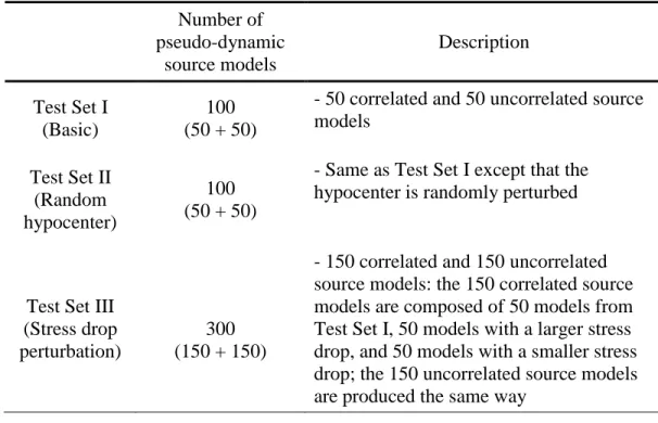
Table 2. Three sets of model tests 494 Number of pseudo-dynamic source models Description Test Set I (Basic) 100 (50 + 50)
- 50 correlated and 50 uncorrelated source models Test Set II (Random hypocenter) 100 (50 + 50)
- Same as Test Set I except that the hypocenter is randomly perturbed
Test Set III (Stress drop perturbation)
300 (150 + 150)
- 150 correlated and 150 uncorrelated source models: the 150 correlated source models are composed of 50 models from Test Set I, 50 models with a larger stress drop, and 50 models with a smaller stress drop; the 150 uncorrelated source models are produced the same way
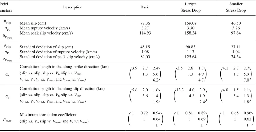
Table 3. Input source statistics model 496
Model
Parameters Description Basic
Larger Stress Drop Smaller Stress Drop 1 -Po in t Statis tics 𝜇𝑠𝑙𝑖𝑝 𝜇𝑉 𝑟 𝜇𝑉 𝑚𝑎𝑥 Mean slip (cm)
Mean rupture velocity (km/s) Mean peak slip velocity (cm/s)
78.36 3.27 114.93 159.08 3.30 158.24 46.50 3.26 97.84 𝜎𝑠𝑙𝑖𝑝 𝜎𝑉𝑟 𝜎𝑉𝑚𝑎𝑥
Standard deviation of slip (cm)
Standard deviation of rupture velocity (km/s) Standard deviation of peak slip velocity (cm/s)
45.15 1.08 89.00 90.83 1.17 125.64 27.11 1.04 74.54 2 -Po in t Statis tics 𝑎𝑥
Correlation length in the along-strike direction (km)
(slip vs. slip, slip vs. Vr, slip vs. Vmax,
Vr vs. Vr, Vr vs. Vmax, and Vmax vs. Vmax)
(3.9 2.71.3 2.45.6 6.2 ) (3.5 2.61.3 1.74.9 4.7 ) (4.1 2.71.3 2.75.9 7.0 ) 𝑎𝑧
Correlation length in the along-dip direction (km)
(slip vs. slip, slip vs. Vr, slip vs. Vmax,
Vr vs. Vr, Vr vs. Vmax, and Vmax vs. Vmax)
( 5.6 2.0 1.6 3.6 1.4 1.9 ) ( 13.3 4.0 3.9 4.2 1.9 2.4 ) ( 4.0 1.5 1.1 3.4 1.3 1.8 )
𝜌𝑚𝑎𝑥 Maximum correlation coefficient
(slip vs. Vr, slip vs. Vmax, and Vr vs. Vmax) (
1 0.72 0.94 1 0.64 1 ) (1 0.811 0.890.69 1 ) (1 0.681 0.960.62 1 )
LIST OF FIGURE CAPTIONS 497
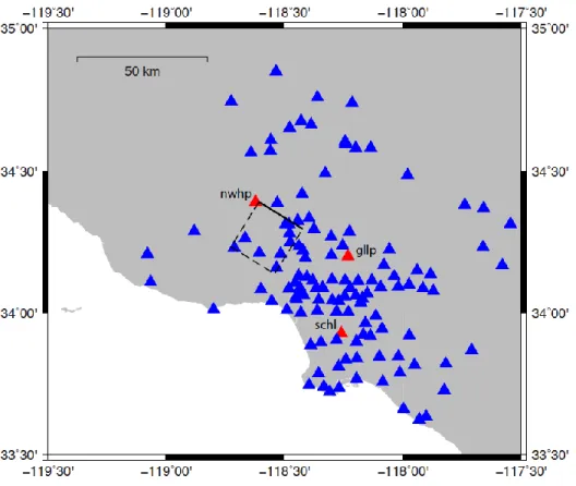
Figure 1. Fault geometry and station locations for the 1994 Northridge, California, earthquake. 498
The black box indicates the ground surface projection of the fault plane; i.e., the top of the fault 499
plane is depicted by a solid line, and the rest of the fault plane is delineated with dashed lines. 500
Triangles show the locations of the 133 stations used in the simulation, including the three 501
selected stations in red. 502
Figure 2. Input correlation model (Test Set I). (a) Correlated, (b) uncorrelated, i.e., without a 503
cross-correlation structure. 504
Figure 3. Correlated pseudo-dynamic source models. The contour lines in the middle panels 505
indicate rupture time distributions. The hypocenter is located at the bottom right corner of the 506
rupture area. 507
Figure 4. Uncorrelated pseudo-dynamic source models. The contour lines in the middle panels 508
indicate rupture time distributions. The hypocenter is located at the bottom right corner of the 509
rupture area. 510
Figure 5. Pseudo-dynamic source models with a larger stress drop. (a) Correlated, (b) 511
uncorrelated. The contour lines in the middle panels indicate rupture time distributions. The 512
hypocenter is located at the bottom right corner of the rupture area. 513
Figure 6. Pseudo-dynamic source models with a smaller stress drop. (a) Correlated, (b) 514
uncorrelated. The contour lines in the middle panels indicate rupture time distributions. The 515
hypocenter is located at the bottom right corner of the rupture area. 516
Figure 7. EASs obtained from Test Set I for the three stations plotted in red in Figure 1. Fifty 517
EAS values are plotted in cyan for each panel. The 50th EAS is added in red as an example. [left]
518
EASs obtained from the correlated pseudo-dynamic source models; [right] EASs obtained from 519
the uncorrelated source models. Both mean and standard deviation from the empirical GMPE 520
model (Bayless and Abrahamson, 2019b) are presented for comparison purposes. 521
Figure 8. Mean residuals between the simulated EASs and those predicted by the empirical 522
GMPE (Bayless and Abrahamson, 2018b). (a) Test Set I (basic), (b) Test Set II (random 523
hypocenter), and (c) Test Set III (stress drop perturbation). 524
Figure 9. Standard deviations (tau: between-event, phi: within-event, and phi0: within-site) of 525
the EAS residuals in (a) Test Set I (basic), (b) Test Set II (random hypocenter), and (c) Test Set 526
III (stress drop perturbation). For the within-event standard deviation from the empirical model, 527
both the within-event (i.e., within-site and between-site terms) and only the within-site standard 528
deviations are presented for the comparison purposes. 529
Figure 10. Inter-frequency correlations (between-event) with 5 reference frequencies (0.2, 0.3, 530
0.4, 0.5, and 1.0 Hz) in (a) Test Set I (basic), (b) Test Set II (random hypocenter), and (c) Test 531
Set III (stress drop perturbation). 532
Figure 11. Inter-frequency correlations (within-event) with 5 reference frequencies (0.2, 0.3, 0.4, 533
0.5, and 1.0 Hz) in (a) Test Set I (basic), (b) Test Set II (random hypocenter), and (c) Test Set III 534
(stress drop perturbation). 535 536 537 538 539 540 541 542
FIGURES 543
544
Figure 1. Fault geometry and station locations for the 1994 Northridge, California, earthquake. 545
The black box indicates the ground surface projection of the fault plane; i.e., the top of the fault 546
plane is depicted by a solid line, and the rest of the fault plane is delineated with dashed lines. 547
Triangles show the locations of the 133 stations used in the simulation, including the three 548
selected stations in red. 549
551
Figure 2. Input correlation model (Test Set I). (a) Correlated, (b) uncorrelated, i.e., without a 552
cross-correlation structure. 553
555
Figure 3. Correlated pseudo-dynamic source models. The contour lines in the middle panels 556
indicate rupture time distributions. The hypocenter is located at the bottom right corner of the 557
rupture area. 558
559
561
Figure 4. Uncorrelated pseudo-dynamic source models. The contour lines in the middle panels 562
indicate rupture time distributions. The hypocenter is located at the bottom right corner of the 563
rupture area. 564
565
567
Figure 5. Pseudo-dynamic source models with a larger stress drop. (a) Correlated, (b) 568
uncorrelated. The contour lines in the middle panels indicate rupture time distributions. The 569
hypocenter is located at the bottom right corner of the rupture area. 570
571
573
Figure 6. Pseudo-dynamic source models with a smaller stress drop. (a) Correlated, (b) 574
uncorrelated. The contour lines in the middle panels indicate rupture time distributions. The 575
hypocenter is located at the bottom right corner of the rupture area. 576
577
579
Figure 7. EASs obtained from Test Set I for the three stations plotted in red in Figure 1. Fifty 580
EAS values are plotted in cyan for each panel. The 50th EAS is added in red as an example. [left] 581
EASs obtained from the correlated pseudo-dynamic source models; [right] EASs obtained from 582
the uncorrelated source models. Both mean and standard deviation from the empirical GMPE 583
model (Bayless and Abrahamson, 2019b) are presented for comparison purposes. 584
585
Figure 8. Mean residuals between the simulated EASs and those predicted by the empirical 586
GMPE (Bayless and Abrahamson, 2018b). (a) Test Set I (basic), (b) Test Set II (random 587
hypocenter), and (c) Test Set III (stress drop perturbation). 588
Figure 9. Standard deviations (tau: between-event, phi: within-event, and phi0: within-site) of 589
the EAS residuals in (a) Test Set I (basic), (b) Test Set II (random hypocenter), and (c) Test Set 590
III (stress drop perturbation). For the within-event standard deviation from the empirical model, 591
both the within-event (i.e., within-site and between-site terms) and only the within-site standard 592
deviations are presented for the comparison purposes. 593
594
Figure 10. Inter-frequency correlations (between-event) with 5 reference frequencies (0.2, 0.3, 595
0.4, 0.5, and 1.0 Hz) in (a) Test Set I (basic), (b) Test Set II (random hypocenter), and (c) Test 596
Set III (stress drop perturbation). The initial decay patterns of both correlated and uncorrelated 597
source models from the reference frequencies, i.e., 0.5 Hz for (a) and (c), and 0.4 Hz for (b), are 598
emphasized with red and blues lines, respectively. 599
600
Figure 11. Inter-frequency correlations (within-event) with 5 reference frequencies (0.2, 0.3, 0.4, 601
0.5, and 1.0 Hz) in (a) Test Set I (basic), (b) Test Set II (random hypocenter), and (c) Test Set III 602
(stress drop perturbation). 603
−119˚30' −119˚30' −119˚00' −119˚00' −118˚30' −118˚30' −118˚00' −118˚00' −117˚30' −117˚30' 33˚30' 33˚30' 34˚00' 34˚00' 34˚30' 34˚30' 35˚00' 35˚00' 50 km nwhp gllp schl Figure 1
slip vs. slip -10 0 10 hx (km) -5 0 5 hz (km)
slip vs. Vr slip vs. Vmax
Vr vs. Vr Vr vs. Vmax Vmax vs. Vmax
(a)
(b)
slip vs. slip -10 0 10 hx (km) -5 0 5 hz (km)slip vs. Vr slip vs. Vmax
Vr vs. Vr Vr vs. Vmax Vmax vs. Vmax 0 0.5 1 Figure 2
slip (cm) -15 -10 -5 0 -15 -10 -5 0 5 Vr (km/sec) 1 1 2 2 3 3 3 4 4 4 5 5 5 5 6 -15 -10 -5 0 -15 -10 -5 0 5 Vmax (cm/sec) -15 -10 -5 0 5 slip (cm) -15 -10 -5 0 -15 -10 -5 0 5 Vr (km/sec) 1 1 2 2 2 3 3 3 4 4 4 5 5 5 5 6 6 7 -15 -10 -5 0 -15 -10 -5 0 5 Vmax (cm/sec) -15 -10 -5 0 5 slip (cm) -15 -10 -5 0 -15 -10 -5 0 5 0 50 100 150 200 250 Vr (km/sec) 1 1 2 2 2 3 3 3 4 4 4 5 5 5 5 6 6 -15 -10 -5 0 -15 -10 -5 0 5 1 2 3 4 5 Vmax (cm/sec) -15 -10 -5 0 5 0 100 200 300 along-dip (k m)
(a) Model 1 (b) Model 2 (c) Model 3 Figure 3
slip (cm) -15 -10 -5 0 -15 -10 -5 0 5 Vr (km/sec) 1 1 2 2 3 3 3 4 4 4 5 5 5 6 -15 -10 -5 0 -15 -10 -5 0 5 Vmax (cm/sec) -15 -10 -5 0 5 slip (cm) -15 -10 -5 0 -15 -10 -5 0 5 Vr (km/sec) 1 1 2 2 3 3 3 4 4 4 5 5 5 5 6 7 -15 -10 -5 0 -15 -10 -5 0 5 Vmax (cm/sec) -15 -10 -5 0 5 slip (cm) -15 -10 -5 0 -15 -10 -5 0 5 0 50 100 150 200 250 Vr (km/sec) 1 1 2 2 3 3 4 4 4 5 5 5 6 6 7 -15 -10 -5 0 -15 -10 -5 0 5 1 2 3 4 5 Vmax (cm/sec) -15 -10 -5 0 5 0 100 200 300 along-dip (k m)
(a) Model 1 (b) Model 2 (c) Model 3 Figure 4
slip (cm) -10 -5 0 -10 -5 0 5 Vr (km/sec) 1 2 2 3 3 3 4 -10 -5 0 -10 -5 0 5 Vmax (cm/sec) -10 -5 0 -10 -5 0 5 slip (cm) -10 -5 0 -10 -5 0 5 0 100 200 300 400 Vr (km/sec) 1 1 2 2 2 3 3 3 4 4 -10 -5 0 -10 -5 0 5 1 2 3 4 5 Vmax (cm/sec) -10 -5 0 -10 -5 0 5 0 100 200 300 400 500
(a)
(b)
along-strike (km) along-dip (k m) Figure 5slip (cm) -20 -10 0 -20 -10 0 Vr (km/sec) 1 2 3 3 4 4 5 5 5 6 6 6 7 7 7 7 8 8 9 10 -20 -10 0 -20 -10 0 Vmax (cm/sec) -20 -10 0 -20 -10 0 slip (cm) -20 -10 0 -20 -10 0 0 50 100 150 Vr (km/sec) 1 2 2 3 3 4 4 4 5 5 5 6 6 6 7 7 7 8 9 10 -20 -10 0 -20 -10 0 1 2 3 4 5 Vmax (cm/sec) -20 -10 0 -20 -10 0 0 100 200 300
(a)
(b)
along-strike (km) along-dip (k m) Figure 610-1 100 101 Freq. (Hz) 101 102 EAS (cm/s) 10-1 100 101 Freq. (Hz) 101 102 EAS (cm/s)
(a) EAS (nwhp)
10-1 100 101 Freq. (Hz) 100 101 102 EAS (cm/s) 10-1 100 101 Freq. (Hz) 100 101 102 EAS (cm/s)(b) EAS (gllp)
100 101 102 EAS (cm/s) 100 101 102 EAS (cm/s)(c) EAS (schl)
Figure 710-1 100 101 Freq. (Hz) -1 -0.5 0 0.5 1 ln Residual
(a) Test Set I
corr no-corr 10-1 100 101 Freq. (Hz) -1 -0.5 0 0.5 1 ln Residual corr no-corr(b) Test Set II
10-1 100 101 Freq. (Hz) -1 -0.5 0 0.5 1 ln Residual corr no-corr(c) Test Set III
Figure 810
-1
10
0
10
1
Freq. (Hz)
0
0.2
0.4
0.6
0.8
1
tau (corr)
phi (corr)
tau (no-corr)
phi (no-corr)
tau (empirical)
phi (empirical)
phi0 (empirical)
Sigma in natural logarithm
(a) Standard Deviation (Test Set I)
Figure 9a10
-1
10
0
10
1
Freq. (Hz)
0
0.2
0.4
0.6
0.8
1
Sigma in natural logarithm
(b) Standard Deviation (Test Set II)
Figure 9b10
-1
10
0
10
1
Freq. (Hz)
0
0.2
0.4
0.6
0.8
1
Sigma in natural logarithm
(c) Standard Deviation (Test Set III)
Figure 9c10-1 100 0.6 0.7 0.8 0.9 1
(a) Between-event correlation (Test Set I)
Correlation Freq. (Hz) 10-1 100 0.6 0.7 0.8 0.9
1 (b) Between-event correlation (Test Set II)
Correlation Freq. (Hz) 10-1 100 0.6 0.7 0.8 0.9
1 (c) Between-event correlation (Test Set III)
Correlation Freq. (Hz) dashed: empirical magenta: correlated cyan: uncorrelated Figure 10
10-1 100 0.6 0.7 0.8 0.9 1
(a) Within-event correlation (Test Set I)
10-1 100 0.6 0.7 0.8 0.9 1
(b) Within-event correlation (Test Set II)
0.6 0.7 0.8 0.9 1
(c) Within-event correlation (Test Set III) Freq. (Hz) Freq. (Hz) Correlation Correlation Correlation dashed: empirical magenta: correlated cyan: uncorrelated Figure 11