S-wave velocity measurements applied to the seismic microzonation of Basel, Upper Rhine Graben

GJI

Seismology

S-wave velocity measurements applied to the seismic microzonation

of Basel, Upper Rhine Graben

Hans-Balder Havenith,

∗ Donat F¨ah,

Ulrich Polom

and Agathe Roull´e

3_{Bureau de Recherches G´eologiques et Mini`eres, BRGM – ARN/RIS, 3 avenue Claude Guillemin, 45060 Orl´eans cedex 2, France}

Accepted 2007 February 23. Received 2007 January 23; in original form 2006 June 28

S U M M A R Y

An extensive S-wave velocity survey had been carried out in the frame of a recent seismic microzonation study of Basel and the border areas between Switzerland, France and Germany. The aim was to better constrain the seismic amplification potential of the surface layers. The survey included single station (H/V spectral ratios) and ambient vibration array measurements carried out by the Swiss team, as well as active S-wave velocity measurements performed by the German and French partners. This paper is focused on the application of the array technique, which consists in recording ambient vibrations with a number of seismological stations. Several practical aspects related to the field measurements are outlined. The signal processing aims to determine the dispersion curves of surface waves contained in the ambient vibrations. The inversion of the dispersion curve provides a 1-D S-wave velocity model for the investigated site down to a depth related to the size of the array. Since the size of arrays is theoretically not limited, arrays are known to be well adapted for investigations in deep sediment basins, such as the Upper Rhine Graben including the area of the city of Basel. In this region, 27 array measurements with varying station configurations have been carried out to determine the S-wave velocity properties of the geological layers down to a depth of 100–250 m. For eight sites, the outputs of the array measurements have been compared with the results of the other investigations using active sources, the spectral analysis of surface waves (SASW) and S-wave reflection seismics. Borehole information available for a few sites could be used to calibrate the geophysical measurements. By this comparison, the advantages and disadvantages of the array method and the other techniques are outlined with regard to the effectiveness of the methods and the required investigation depth. The dispersion curves measured with the arrays and the SASW technique were also combined and inverted simultaneously to use the advantages of both methods. Finally, the paper outlines and discusses the contribution of the S-wave velocity survey to the new seismic microzonation of the Basel region. In this regard one major outcome of the survey is the quantification of vertical and lateral changes of the S-wave velocity, due to changing lithology or changing compaction and degree of weathering of the layers. Key words: array method, Basel, surface wave analysis, S-wave velocity model, Switzerland, Vs variability.

I N T R O D U C T I O N

For seismic microzonation purposes, the average S-wave velocity of the upper 30 m, Vs30, is often considered as key parameter for the assessment of site effects. It is, however, questionable if the Vs30 sufficiently characterizes the local amplification potential in some particular geological environments, such as deep

sediment-∗Now at: ETH Zurich, Institute of Geophysics, Swiss Seismological Service, ETH Hoenggerberg, HPP L6, 8093 Zurich, Switzerland.

filled basins. In many cases it was shown that deeper layers may also significantly contribute to amplification effects over a broad frequency range between 0.1 and 10 Hz. Examples from western Europe include the Upper (Kind 2002) and Lower Rhine Graben (Scherbaum et al. 2003; Hinzen et al. 2004; Parolai et al. 2006), the Grenoble basin (Cornou et al. 2003), the Rhone valley (Roten et al. 2006) and the northern part of the Brabant massif covered by loose sediments (Nguyen et al. 2004; Wathelet et al. 2004). The recognized influence of the deeper geology on the seismic ground motion behaviour at the surface implies a major challenge: the need of developing geophysical techniques able to provide reliable in-formation on the dynamic behaviour over a large range of depths.

A typical deep penetration method is the seismic reflection tech-nique, using an active source producing compressive and/or shear waves. The S-wave reflection technique is preferentially used for earthquake engineering purposes since it allows to map also lateral variations of the structure (Polom et al. 2005).

An alternative method based on passive seismic sources, for ex-ample, microtremors, has been under research since the pioneering works of Aki (1957), Capon (1969) and Lacoss et al. (1969). They showed that ambient noise recorded by seismological arrays of vari-able size includes sufficient information to invert the S-wave velocity structure. The information is provided by the dispersive behaviour of surface waves, which constitute a major part of the ambient noise. The spectral analysis of surface waves (SASW) induced by active sources is an additional technique able to provide information on the shear wave properties of the underground. A comprehensible review of various surface wave techniques is given by Tokimatsu (1997). With regard to active seismic techniques, the array method is known to be more cost effective and to be less affected by uncorrelated noise (Kind et al. 2005). For two sites (Kannenfeld and Grenzach outlined in Fig. 1), Vs profiles obtained by the array, SASW and S-wave re-flection methods will be shown. A critical point discussed in this paper is the investigation depth of the applied techniques and the resolved layer thickness.

In Europe, a major effort to develop this so-called array technique was made in the frame of the now completed EU project Site Ef-fects Assessment using Ambient Excitations (SESAME) (SESAME 2005). One goal of this project was to develop a software treating both the analysis of the noise records and the inversion of dispersion curves (Ohrnberger 2004; Wathelet et al. 2004, 2005; Kind et al. 2005). The know-how acquired during this project was used in or-der to improve the efficiency and quality of our measurements in the region of Basel.

M I C R O Z O N AT I O N O F B A S E L

The seismic hazard of Switzerland can be described as moderate with PGA values of 0.1–0.16 g not exceeded in 50 yr with a prob-ability of 90 per cent (Giardini et al. 2004). However, several large earthquakes (with Mw> 6) have occurred in the past. In particular, Basel was severely damaged by the 1356 earthquake (EMS inten-sity IX), the largest among a series of events affecting the south-ern Upper Rhine region during the last millennium. The location of the city of Basel within a deep sedimentary basin, the Upper Rhine Graben (Fig. 1), with a large amplification potential adds to the relatively high level of seismic hazard. A general overview of the geology and tectonics in the Basel area is given in F¨ah et al. (1997) and Noack et al. (1997). Here, only a brief description of the geological context will be provided. The city of Basel is close to the Eastern Rhine Graben fault (indicated in Fig. 1) with a throw of about 1400 m. Within the Rhine Graben (on the down-thrown side), the Mesozoic strata (Triassic to Jurassic) are covered by 500– 1000 m of Tertiary sediments. They form an asymmetric syncline (steeper eastern limb) with its axis parallel to the fault zone (see Fig. 1). These Tertiary layers are known only by very few outcrops and deep reaching wells. The following Tertiary formations can be distinguished: the mostly argillaceous marls of the Melettalayers, (maximum 350 m thick), which become more sandy at its transition to the ‘Molasse Alsacienne’ (see Fig. 1b). The ‘Molasse Alsaci-enne’, with a maximum thickness of 300 m, is an intercalation of sandy layers and argillaceous marls. The topmost ‘T¨ullinger layers’ (maximum 200 m thick, not present along the section in Fig. 1b) are

calcareous to argillaceous marls with interlayering freshwater car-bonates. Above the Tertiary sediments, 5–40 m of Pleistocene and Holocene gravels were deposited, mostly by the river Rhine. The composition of these gravels is well known throughout the urban area by about 3000 shallow wells. To the east, on the shoulder of the Rhinegraben, Palaeozoic layers (Rotliegendes) and the Mesozoic sediments (Schilf Sandstone, Keuper Gypsum and Muschelkalk in Fig. 1b) of the Tabular Jura are covered directly by 5–50 m of Qua-ternary (Pleistocene and Holocene) gravels.

To address the issue of seismic hazard and microzonation in the Basel region, several research projects had been carried out (F¨ah

et al. 1997, 2001a; Kind 2002; Steimen et al. 2004). Part of the

research was focused on investigating the local site conditions in Basel and on analysing the vulnerability of the buildings in the city. The projects resulted in a qualitative (determination of zones using geological information and fundamental frequency, f0, mea-surements) and quantitative (with determination of zone-specific re-sponse spectra) seismic microzonation. The quantitative microzona-tion performed for the city of Basel is based on borehole informamicrozona-tion and a derived geological 3-D model (Kind 2002), five S-wave veloc-ity measurements using the array method, several hundreds of H/V measurements and numerous 2-D simulations of seismic ground motion amplification.

This microzonation was revised in the frame of an Interreg project ‘Seismic Microzonation of the Southern Upper Rhine’ and com-pleted in 2006. The site investigation included additional H/V mea-surements (more than 1000 done by German, French and Swiss partners) and new S-wave velocity surveys. The surveys comprised array measurements (Schweizerischer Erdbebendienst, SED, ETH Zurich), SASW (Bureau de Recherches G´eologiques et Mini`eres, BRGM, France) as well as S-wave reflection and refraction seis-mics and a few geophysical tests in boreholes (Institut f¨ur Geowis-senschaftliche Gemeinschaftsaufgaben, GGA, Germany).

Here, we will principally describe the array measurement surveys and compare related results with the outputs of the other types of investigations. At the end, it will be shown how these new surveys contributed to a more precise characterization of the shear wave properties of the different investigated geological materials and to the new seismic microzonation of the target area.

A R R AY M E A S U R E M E N T S — F I E L D E X P E R I E N C E S

Twenty-seven sites were investigated with the array technique. The sites were selected in order to get information on the seismic proper-ties of all relevant geological materials within and outside the main graben structure (Fig. 1). The types of investigated layers include compacted Tertiary and Mesozoic sediments generally covered by loose quaternary deposits, that is, loess, sand and clay or gravels (see Table 1 in the annex). The measurements were performed during the winter season 2004–2005, at daytime, along the valley bottom, on hilltops and slopes, in the centre of the city and in agricultural areas. A series of different array configurations made of 5–9 seismologi-cal stations (Lennartz 5 s three-component seismometers connected to 24 bit Quanterra or 16 bit Mars88 stations) were tested in the field. This included crosses, triangles, pentagons and hexagons or mixed configurations (Fig. 2). At each site, at least two arrays with different apertures (array radius) were set up (Fig. 2); each of them characterized by similar interstation distances (or multiples of these distances). In the following, these single arrays will be called sub-arrays or rings. All subsub-arrays included one (see Fig. 2a) or more

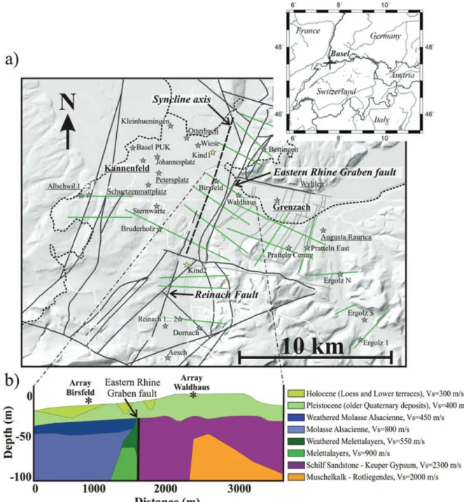
Figure 1. Twenty-five metre-resolution digital elevation model of the southern Upper Rhine Graben with country (dashed lines) and canton borders (white

lines), the main graben structure (dark grey lines) with rough outline of syncline axis (dashed line) and the graben and horst structure (light grey lines) in the east of the Eastern Rhine Graben fault (shown). Array sites are outlined by filled stars (yellow stars are arrays performed by Kind 2002); names of array sites investigated also by SASW profiles and S-wave reflection and refraction profiles are underlined. In green the geological–geophysical cross-sections used for numerical simulations are outlined. The two sites analysed more in detail in this paper are Kannenfeld (inside the graben) and Grenzach (in the east of the main graben). A geological section across the Eastern Rhine Graben fault with indication of Vs-properties of the different units is shown in (b). It shows Palaeozoic (Rotliegendes), Mesozoic (Muschelkalk, Schilf Sandstone and Keuper Gypsum), Tertiary (Melettalayers and ‘Molasse Alsacienne’) and Quaternary (Holocene and Pleistocene) layers.

(30 m triangle of four stations in Fig. 2b) common central stations. The smallest used subarrays had an aperture of 10–30 m; the aperture of each of the following subarrays was increased two to three times. The meaning of this factor will be discussed below. The recording time of the small subarrays was about 30 min and more than 1 hr for the larger ones (>50 m aperture). This way of doing had been sug-gested by several partners of the SESAME project after a series of completed tests in the field (SESAME 2005). They showed that each

subarray provides reliable information on the dispersion of surface waves over a limited frequency range related to the size of the sub-array: records of small subarrays contribute to the dispersion curve at higher frequencies, records of the large subarrays contribute to the dispersion at lower frequencies.

For the previous microzonation of Basel, Kind (2002) had ap-plied another procedure of array measurements: he built a single large array with more than 10 stations, maximizing the number of

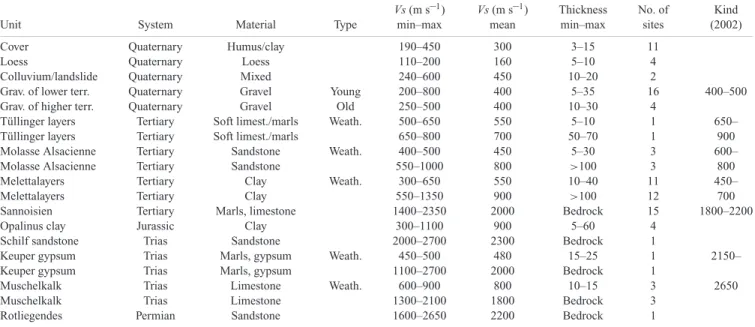
Table 1. Vs-properties of the geological materials determined by Array measurements.

Vs (m s–1_{) Vs (m s–}1_{) Thickness No. of Kind}

Unit System Material Type min–max mean min–max sites (2002)

Cover Quaternary Humus/clay 190–450 300 3–15 11

Loess Quaternary Loess 110–200 160 5–10 4

Colluvium/landslide Quaternary Mixed 240–600 450 10–20 2

Grav. of lower terr. Quaternary Gravel Young 200–800 400 5–35 16 400–500

Grav. of higher terr. Quaternary Gravel Old 250–500 400 10–30 4

T¨ullinger layers Tertiary Soft limest./marls Weath. 500–650 550 5–10 1 650–

T¨ullinger layers Tertiary Soft limest./marls 650–800 700 50–70 1 900

Molasse Alsacienne Tertiary Sandstone Weath. 400–500 450 5–30 3 600–

Molasse Alsacienne Tertiary Sandstone 550–1000 800 >100 3 800

Melettalayers Tertiary Clay Weath. 300–650 550 10–40 11 450–

Melettalayers Tertiary Clay 550–1350 900 >100 12 700

Sannoisien Tertiary Marls, limestone 1400–2350 2000 Bedrock 15 1800–2200

Opalinus clay Jurassic Clay 300–1100 900 5–60 4

Schilf sandstone Trias Sandstone 2000–2700 2300 Bedrock 1

Keuper gypsum Trias Marls, gypsum Weath. 450–500 480 15–25 1 2150–

Keuper gypsum Trias Marls, gypsum 1100–2700 2000 Bedrock 1

Muschelkalk Trias Limestone Weath. 600–900 800 10–15 3 2650

Muschelkalk Trias Limestone 1300–2100 1800 Bedrock 3

Rotliegendes Permian Sandstone 1600–2650 2200 Bedrock 1

Figure 2. Measurements done at Kannenfeld (a) and Grenzach (b). Grey

points show the station position within the arrays, the circles outline the subarray rings with a certain aperture; the open triangles show the centres of the SASW profile, the dotted lines indicate the S-wave reflection and refraction profiles. The open squares in (a) show the station location of the array done by Kind (2002).

different interstation distances (small and large distances, configu-ration compared in Fig. 2a). On the basis of a direct comparison it will be shown which of the two techniques is more efficient, the sin-gle large array or the subarray method. First, the subarray technique is obviously cheaper and ‘lighter’ since it requires fewer stations as well as related acquisition and transportation costs. On the other hand, the total recording time of a series of subarrays is larger than for a single array: about 1 hr for a single large array, and at least 2 hr for two or three subarrays. Then, the accurate measurement of the station positions takes more time if subarrays are used since the total number of different station positions is larger than for a single array. According to our experience, the geodetic measurements in densely inhabited areas with limited open spaces (a typical case of application of the array technique) could require more than 50 per cent of the entire fieldwork time. This is due to the required high precision of the positioning; the maximum position measurement error should be less than 1 per cent of the array aperture: for exam-ple, less than 20 cm for a subarray with a 20 m aperture. For small to medium-size arrays, this requires the use of total station (theodo-lite) or differential GPS (DGPS). For very large arrays (aperture> 500 m) a simple GPS is sufficient. The DGPS technique is in general less time-consuming than total station, but its application is severely constrained by the quality of the satellite signal reception. In many cases of measurements, particularly in towns, between houses or below trees in parks, the signal quality is poor and does not allow a precise measurement.

Thus, it can be concluded that a single array measurement is more interesting in towns if economical aspects are disregarded. In remote areas, however, the lighter subarray technique can be better adapted to the difficult field conditions and thus is clearly more efficient. This could be inferred from our recent experience of array measurements in the Tien Shan Mountains, Central Asia (Havenith et al. 2006).

Below we will discuss the quality and reliability of the results obtained by the respective techniques applied at the same sites.

O T H E R I N V E S T I G AT I O N M E T H O D S

At eight sites, array measurements were complemented by SASW,

infers the Vs-model from the dispersion of Rayleigh waves induced by an active seismic source and wave propagation recorded along a profile. For the measurements in Basel, the French partner BRGM used a sledgehammer as source; the seismic signals were recorded along 96-m long profile made of 48 10 Hz-geophones. Due to the limited source energy, profile length, and natural frequency of the geophones, the SASW method works within a higher frequency range (typically 10–60 Hz) than the array technique (typically< 20 Hz) and is better adapted to define the Vs-structure of the shallow layers (down to a maximum of 40 m). The S-wave reflection and refraction measurements were carried out by the German group GGA using a horizontally vibrating device shearing the ground in order to excite S waves (Polom et al. 2005). The S waves are recorded along a 94-m long profile (in some cases the profiles were longer) of horizontal 10 Hz geophones with 1 or 2 m spacing within a frequency range of 10–200 Hz. This allows for high resolution imaging of the shallow subsurface and for a deep penetration down to 100 m and more (Polom et al. 2005). Where possible, the GGA had also carried out direct P- and S-wave velocity measurements in boreholes in order to validate the surface investigations.

Before comparing the results of the SASW, array and S-wave reflection–refraction survey, we briefly summarize some practical aspects of the field measurements. In the field, the SASW method is ‘lighter’ than the two other methods and several sites can be inves-tigated in 1 day by two geophysicists (Polom et al. 2005); the pro-cessing of those data requires another few days. Array and S-wave reflection methods are equally laborious: one or two sites could be studied per day by two or three investigators; and at least 1 day is required for the processing of the data collected at one site. A major drawback of the array technique is the time required for the laborious geodetic measurements of the station positions. Actually, the other measurements are performed along profiles with fixed length and known geophone spacing (depending on the spreads); only, an in-significant amount of time is needed to define the relative geophone position. Within an array the positions of the single stations are not fixed and have to be measured with high precision; as mentioned above, up to 50 per cent of the total field work time may be spent on those measurements. A significant improvement of the system would be reached if the stations could be positioned automatically; this aspect is now under research.

From the point of view of signal quality, array records and their processing revealed to be the least affected by uncorrelated noise.

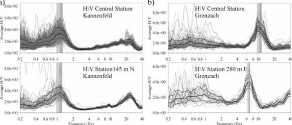
Figure 3. Examples of H/V ratios (grey) for two stations of the Kannenfeld (a) and the Grenzach (b) arrays. Average and one standard deviation ratios are

marked by solid black and dashed black lines, respectively.

As expected, this was particularly true for measurements in densely inhabited areas.

A R R AY M E A S U R E M E N T S — D AT A P R O C E S S I N G

The processing of the noise data can be subdivided into pre-processing (1), extraction of the dispersion curve (2) and inversion of the curve in order to obtain the Vs-model (3).

The pre-processing (1) consists in the re-formatting of the data, computation of the station position and construction of a ‘subar-ray signal database’ with the GEOPSY tool developed by Wathelet (2005) in the frame of the SESAME project. GEOPSY also allowed us to compute the horizontal by vertical signal ratios. These so-called H/V ratios were evaluated for all station sites of the array and compared with each other. On the basis of the f0shown by the H/V ratios, the 1-D structure of the underground—the required condi-tion for reliable measurements outputs—could be verified. Stacondi-tion records characterized by fundamental frequencies differing signif-icantly from the others were not used for the extraction of the dis-persion curve. Examples of similar and dissimilar H/V ratios are shown in Fig. 3.

For the study presented here, only the dispersion of Rayleigh waves was analysed on the basis of the vertical component records. Recently, we started to work also with the horizontal compo-nents, analysing both Rayleigh and Love surface waves (F¨ah et al. 2007).

The records of each ‘subarray signal data base’ were analysed with the high-resolution beam forming frequency-wave number (F-K) method developed by Capon (1969). The dispersion curve was determined by the maximum energy within the F-K spectrum. The processing was done with two different programs implementing this technique, the Array Tool developed by Kind et al. (2005) and CAP (Ohrnberger 2004), which is part of the GEOPSY package. The CAP software also includes other array analysis tools (SPAC: Aki 1957; MUSIC: Schmidt 1981; among others), which were not used for this study.

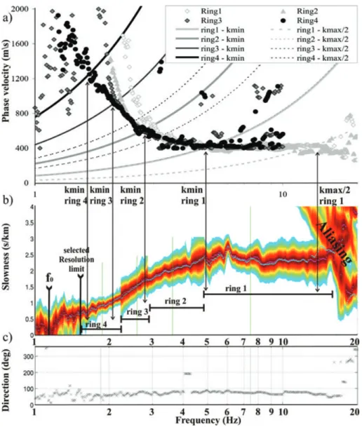
The output of the F-K computation can be visualized in terms of dispersion diagram, picked dispersion curve and direction-frequency graph of the incoming most energetic waves. Fig. 4 shows an example of the output of the Kannenfeld array processing. From the direction-frequency graph in Fig. 4(c) it can be observed that,

Figure 4. Dispersion diagram for the Kannenfeld array combining the diagrams obtained for the four subarray rings. (a) Dispersion curves (energy crest in

b, here in m s–1_{-Hz) of the four rings with indication of the relative k}

minand kmax/2 limits of the computed array response. (b) Energy dispersion diagram

(s km–1_{-Hz) for analysed Rayleigh waves and selected parts of the dispersion diagram of each ring. (c) Graph showing the direction of the incoming most}

energetic surface waves.

at this site, most of the Rayleigh wave energy is coming from the east–northeast (60–80◦), that is, from the Rhine River and the cen-tre of the town. The dispersion of this energy is represented in the slowness-frequency diagram in Fig. 4(b). The crest of the energy distribution constitutes the so-called dispersion curve; the width of the crest provides some indication on the uncertainty of the de-termined dispersion curve. In the case shown in Fig. 4b, the en-ergy crest is quite narrow and the corresponding dispersion curve could be defined with a high degree of certainty. The same degree of certainty was, however, not reached for all the 27 investigated sites.

Note the diagram in Fig. 4(b) is, actually, composed of the dis-persion graphs computed for the four subarrays (rings) represented in Fig. 2(a).

From the corresponding four subarray dispersion curves we ex-tracted relevant parts, between aliasing at high frequencies and loss of resolution at lower frequencies, and connected them with each other. The selection of the different parts was validated by the com-parison with the minimum and maximum wave number limits (kmin

and kmax/2) determined from the theoretical response of each sub-array. kmindefines the resolution limit of the array geometry and is measured at the mid-height of the central peak of the theoretical ar-ray response. kmaxdefines the aliasing limit and is set where the first aliasing peak exceeds 0.5. As recommended by Wathelet (2005) we used only the parts between kmin and kmax/2. The Kannenfeld array analysis shown in Fig. 4 reveals that the selected parts (Fig. 4b) correspond more or less to the interval between the com-puted kmax/2 and kmin(Fig. 4a); they are, however, exceeding the kmin of the largest ring and theoretical kmax/2 of the smallest ring. In this regard it should be mentioned that the kmax/2 is a quite conservative limit and it will be shown in the following that also data beyond this limit may be valuable. On the other hand, from our experience we know that the kminshould be strictly respected; often, this limit is exceeded to cover a lower frequency range and enhance the possible penetration depth; however, related results must be considered as less reliable. The problem related to the use of values below kminis exemplified in Fig. 4(a) by the fast increase of measured Vs in the dispersion curve for the small and intermediate sized rings.

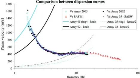
Figure 5. Dispersion curves obtained by array analysis (Kind 2002, black diamonds; array 2005, open blue circles) and SASW (open red triangles) for the

Kannenfeld site. The joined array—SASW dispersion curve is marked by small purple crosses. The dashed lines represent the kmax/2 functions, the thick

continuous lines the kminfunctions for the array 2005 (blue) and Kind 2002 (black).

Concerning the definition of the dispersion curve within the phase velocity (or slowness)—frequency diagram, two practical aspects should be pointed out. First, we observed that all applied array con-figurations with six or more operative stations performed equally well in producing the dispersion diagram; arrays with less than six stations did generally not allow us to retrieve a clear disper-sion curve. Thus, it can be concluded that the most effective con-figurations consist of six to seven stations distributed within the site infrastructure (crossing roads, pathways and squares). Second, we noticed that the dispersion curves are poorly defined for sites with strong lateral changes: for example, the two outer rings at the Grenzach site crossing a graben and horst structure could not be used for the dispersion analysis—this is also shown by the dissimilar H/V ratios shown in Fig. 3(b).

Once dispersion curves are joined, the combined curve is used as input for the determination of the S-wave velocity model through data inversion. The entire dispersion curve obtained from the array measurement at Kannenfeld is compared in Fig. 5 with the dis-persion data of Kind (2002) and those produced by SASW. From this comparison it can first be observed that the dispersion curves obtained at different times and with different array techniques are quite similar. It is also interesting to notice that the dispersion data produced by Kind (2002) seem to be valuable well beyond the the-oretical kminand kmax/2 limits: they are very similar to the recently acquired data within the respective kminand kmax/2 limits. This could be due to the used high-resolution beam forming frequency-wave number method (Capon 1969), which should be limited primarily by the signal-to-noise ratio of the data and secondarily by the beam pattern of the array.

Fig. 5 further shows that SASW data cover a range of much higher frequencies than the array data. In the overlapping interval between 12 and 15 Hz, both data sets agree reasonably well with each other and could be joined to form one single dispersion curve; this curve was also used for a Vs-model inversion.

The inversion processing was done both with the software in-cluded in the GEOPSY package (na-viewer developed by Wathelet 2005) and the inversion program of the array tool developed by F¨ah

et al. (2003). These two inversion programs are based on the

com-putation of a large number of models that may explain the data. For model generation and selection, na-viewer uses a neighbourhood

algorithm (see Wathelet et al. 2004), while the inversion array tool applies a genetic algorithm. In order to better constrain the depth of the sediment cover, Scherbaum et al. (2003) and F¨ah et al. (2001a, b, 2003) suggest using the ellipticity of the Rayleigh waves provided by the H/V curve as complementary input. Therefore, in addition to the single inversion on the dispersion curve, combined inversions were carried out using also the ellipticity data of the central station.

C O M PA R I S O N B E T W E E N V s - M O D E L S

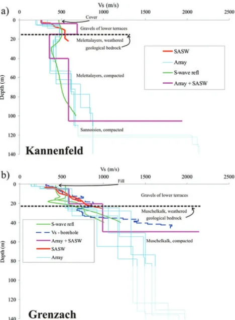
For the Kannenfeld and Grenzach sites, Vs-models produced with the array and the other investigation techniques are shown in Figs 6(a) and (b). First, it should be noted that only one Vs-profile per site was provided by the SASW and S-wave reflection studies, while the inversion of array data produced different possible models allowing us to have a rough estimate of the degree of certainty of the outputs (light blue models in Fig. 6).

Comparing the different models with each other, it can be ob-served that the array measurements provide the deepest Vs-models, and SASW the shallowest. Due to the averaging of the velocity– depth profiles over the measured 2-D section, the S-wave reflection velocity–depth models are smoother than those produced by surface wave inversion. These two general aspects were also observed for the other six sites investigated by all three methods. For the Grenzach site, the Vs investigation in the borehole (Vs borehole in Fig. 6b) can be considered as reference for the velocities of the different units (but not for the lateral variability of the thickness shown in Fig. 3b by the varying H/V spectral ratios). From Fig. 6(b) it can be observed that almost all Vs-models fit more or less this reference

Vs-borehole model: the SASW allows for the best determination of

the thickness of the shallow layers down to 25 m while the inver-sion outputs of the array data fit the direct Vs measurements from 4 to 35 m of depth. The Vs model of the joined SASW and Array dispersion curve inversion is in agreement with the reference model over the entire depth range from the surface down to the bedrock at 40–50 m. While the trend of the Vs-model produced by S-wave reflection seismics compares well with the other Vs-models, it also shows a velocity inversion zone (decreasing velocity with depth) at 20 m depth that is not revealed by SASW and array results. The

Figure 6. Vs models by S-wave reflection (green), array (blue), SASW (red) and joined array+ SASW (purple) analyses for the Kannenfeld (a) and Grenzach

(b) sites with corresponding geological log. In (b), direct Vs measurements in a borehole (dashed black) are compared with the other Vs models. The non-reliable parts are partly masked.

reference Vs-model from borehole data also presents a slight veloc-ity inversion but at a depth of 30 m. This is not shown by the S-wave reflection profile; and, due to the limited investigation depth and single vertical component measurements (no information from pos-sible Love waves allowing for resolving more complex structures as discussed below), it is not indicated by the SASW profile; due to the wavelengths involved, the velocity inversion of such small dimension could neither be resolved by the array method.

A velocity inversion zone is, however, well outlined both by the array and S-wave reflection data for the Kannenfeld site at a depth of 16–40 m (Fig. 6a). Note, the SASW measurements do again not show this velocity inversion due to the limited investigation depth. Considering the array data alone, one should take care when inter-preting them in terms of an inversion zone. First, a velocity inversion may also be an artefact produced by the processing if the parameter variation is not sufficiently constrained during the data inversion process. Here, the dispersion curve clearly shows a slight velocity inversion between 7 and 20 Hz. Thus, the velocity inversion

pre-sented by the model is not due to this artefact. However, in case of such a velocity inversion shown by the data, there is still a possi-bility of mode jumping and misinterpretation of model branch (a dominating higher mode is interpreted as fundamental mode, Toki-matsu 1997). Indeed, for other sites the combined processing of Love and Rayleigh wave dispersion curves revealed that the fundamen-tal and first higher modes (close to the fundamenfundamen-tal mode) could merge and produce an apparent velocity inversion. In this case, the combined processing of Love and Rayleigh wave dispersion curves confirmed the presence of the high velocity layer at a depth of 4–16 m (analysis presented in F¨ah et al. 2007). Since this observation of a velocity inversion from the array Vs-models is also confirmed by the S-wave reflection data, we consider this velocity inversion as indication for a real decrease of the Vs below 16 m depth, that is, on top of the Melettalayers below the gravels of the lower terraces— most probably due to the strong weathering of the Melettalayers. The Vs variation across this velocity inversion is, however not well constrained and source of significant uncertainty.

At shallow depth, both at Kannenfeld and Grenzach, the SASW results agree very well with the low Vs shown by the array

Vs-models. Actually, at almost all sites, the surface wave

meth-ods revealed lower velocities close to the surface than the S-wave reflection seismic prospecting. Note, a similar observation has been made by Boore and Brown (1998) comparing results obtained by Rayleigh-wave methods (using active sources and noted CXW in their paper) with direct borehole measurements. The CXW measure-ments systematically produced lower Vs values for shallow depths, but larger values beyond a depth of 10–20 m. In our study, high Vs were only revealed by array Vs-models beyond a depth of 100 m; this is likely to be related to the greater investigation depth of this method.

Finally, comparing the Vs-profiles in Figs 6(a) and (b), it can be seen that the different Vs-values at a depth of more than 20 m are due to the presence of different lithologies: soft Melettalayers (clay) in Kannenfeld, inside the Rhine graben and significantly harder Muschelkalk (limestone) in Grenzach, outside the main graben. Also the weathered part of the Muschelkalk can be considered as more compact than the Meletta clays.

C O N T R I B U T I O N O F T H E V s - S U RV E Y T O T H E M I C R O Z O N AT I O N O F T H E B A S E L A R E A

Above we presented and discussed method-dependent differences between the Vs models. For microzonation purposes, site-dependent differences need to be outlined and quantified. Despite the variabil-ity of the Vs models at one site, a clear difference can be noticed between the changing S-wave velocity at Kannenfeld (Fig. 6a) and at Grenzach (Fig. 6b). The first site is inside the main graben struc-ture, the second outside; consequently, the geological bedrock is deeper and the sediment cover thicker at the Kannenfeld site. There the Vs does not exceed 800 m s–1_{(characterizing bedrock class A} according to Euro-code 8) up to a depth of more than 100 m where the velocity rises—most probably due to the presence of Sannois-ien limestone. In Grenzach, in the east of the main graben, 800– 1000 m s–1 _{are already met at a depth of about 20 m. The lower} thickness of the sediment cover at Grenzach site is validated by the much higher f0—between 6 and 10 Hz compared to 1.2 Hz at Kannenfeld.

The total variation of the Vs characteristics over the target area can be related to two factors: first, the laterally varying geology (lithol-ogy and tectonics) within and outside the graben and second, the variation of the Vs within one geological layer. In order to assess the first type of changes, measurements had been carried out on a large number of sites inside and outside the graben with thick or shal-low Cenozoic and Mesozoic sediments, on hilltops covered by loess and/or older gravel deposits, river valley bottom filled with younger gravel sediments, along slopes, etc. The investigated lithologies and their Vs characterisation are summarized in Table 1.

The lateral Vs variation inside the same layer can first be related to the degree of weathering of the geological layers. The zone on top of the layers systematically presented significantly lower Vs values than the deeper part of the same layer. These zones are consid-ered as weathconsid-ered part of the layer (see characteristics of weathconsid-ered rocks in Table 1). This interpretation is validated by observations in boreholes (e.g. Grenzach). The effect of weathering on the Vs properties of the layers is particularly evident where these layers are outcropping or close to the surface. As a consequence, the material classified as geological bedrock might not have the strength required

for a geophysical bedrock (type class A, Vs> 800 m s–1_{) as it is} shown both for Kannenfeld and Grenzach in Fig. 6.

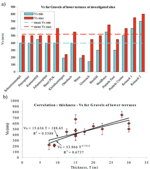
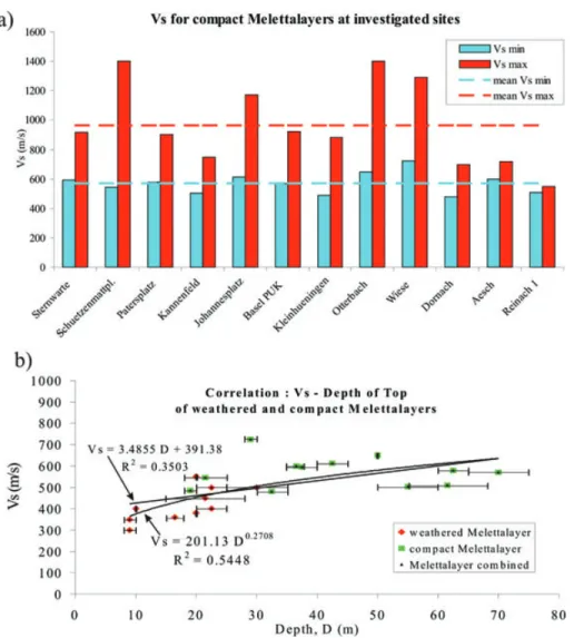
Secondly, lateral Vs changes within the same layers can also be related to their respective thickness. Figs 7 and 8 show such changes within the lower terrace gravels and the clayey Melettalayers inves-tigated, respectively, at 16 and 12 sites. For both layers, the maxi-mum and minimaxi-mum velocity estimates are presented as well as the average upper and lower values. Maximum and minimum values generally correspond to the measured Vs at the bottom and on top of the layer, respectively. From the graph in Fig. 7 it can be inferred that thicker gravel deposits are characterized by higher average Vs. This can also be observed for the other Quaternary layers (cover, Loess, colluvium, gravels of higher terraces in Table 1), but may not be quantified due to the low number of investigation points. In addition, it was noticed that the Vs of the layers changes with the depth of the top of the layers, that is the thickness of the sediment cover. Fig. 8(b) presents related results for the weathered and com-pact Melettalayers. Both, changes of the average Vs properties as a function of layer thickness and depth of layer top can be explained by the dependency of Vs on the degree of compaction of the mate-rial due the weight of the overlaying matemate-rial. In both cases, the best theoretical fit of the correlation between Vs and thickness and depth of layer top is a power law of the type y= axb_{. Such type of law} was also used to characterize the vertical P- and S-wave velocity variation within the Lower Rhine Graben close to Cologne (Budny 1984; Scherbaum et al. 2003). As can be seen from Figs 7b and 8b, this law is marked by a slightly larger increase of Vs for smaller thickness (or depth) values; the function tends to flatten for larger thickness (or depth) values. It should be noted that laws with the same behaviour, for example, logarithmic law, also produce a good fit while the fit by a linear law is slightly worse (see for compar-ison the linear fits presented in Figs 7b and 8b). From this it can be inferred that the changes of Vs with thickness or depth of the same layer are more prominent at shallow depths, at less than 40 m. Hence we may also conclude that changes of Vs at greater depths are mostly due to changing geology (lithology and tectonics) such as shown by the comparison between the Vs-models at Kannen-feld and Grenzach (Figs 6a and b). However, due to the uncertainty affecting the data (see error bars shown in Figs 7b and 8b), fur-ther investigation is necessary (and planned) to better constrain this observation.

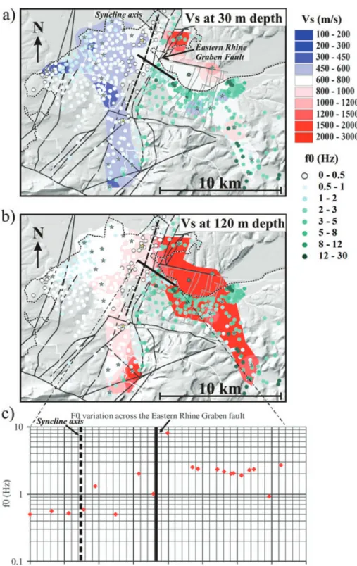
An overview of the Vs variation within the target area is given by Fig. 9a and b. These maps show interpolated Vs values from array measurements at 29 and 24 sites (both including 2 arrays done by Kind 2002 and marked by yellow stars) at a depth of 30 and 120 m, respectively. Comparing these maps with the overlaid points of fun-damental frequencies (see values according to colour scale) and the tectonic structure, it can be observed that some correlation exist be-tween the two latter and the Vs at 120 m depth. A correlation with the Vs at 30 m is not straightforward. This is likely to be due to the influence of the deeper Tertiary layers within the main graben on the lowering of the Vs values at 120 m depth and fundamental frequency. The effect of the low-velocity Tertiary layers in the west of the Eastern Rhine Graben fault on the f0is also clearly shown by the plot of f0(Fig. 9c). Further, it can be seen that the presence of the syncline affects on the f0; along the syncline and in the west of its axis the lowest f0values were obtained; between the axis and the Eastern Rhine Graben fault the f0values are increasing due to decreasing depth of the sediments layers. In the east of the fault, the f0 values are generally above 2 Hz. Outliers both in the east and west of the fault might be due to misinterpretation of the H/V peak or due to locally varying structures. It can be noticed that the

Figure 7. Measured Vs (from array data only) of the lower terrace gravels at investigated sites with estimates of average maximum and minimum values (a)

and correlation between Vs (average value for the layer with error bars corresponding to interval between minimum and maximum Vs estimates) and layer thickness with plot and equation of linear and power-law fits (b).

syncline does not seem to have any influence on the Vs variation, while changes across the Eastern Rhine Graben fault are obvious. These changes of Vs and the f0are of prime importance for seismic microzonation studies.

Summarizing, the major outcome of the entire S-wave velocity survey for the seismic microzonation of the Upper Rhine graben is the quantification of the lateral and vertical changes of Vs as a function of lithology, layer thickness and weathering. From the experience in the modelling of earthquake ground motion it can be inferred that both surface and deeper layers contribute to ground motion amplification. Such simulations further show that the lateral changes of Vs properties are responsible for significant variations of the amplification potential due to the excitation of local surface waves and shaking resonance.

C O N C L U S I O N S

This study is part of a geophysical survey performed in the frame of a new microzonation study of the Basel area located in the Upper Rhine Graben region. The survey aimed at the better

characterisa-tion of the S-wave properties of the local geology and, thus, at a more precise determination of the site amplification potential. Therefore, different Vs-techniques were applied: passive surface wave measure-ments with seismological arrays, active surface wave measuremeasure-ments (SASW), and S-wave reflection and refraction investigations. This paper focuses on the application of the array technique and outlines several practical aspects related to the field measurements; it also describes the procedure applied to derive the dispersion curve and the Vs-models through data inversion.

During the field campaign in 2005, we applied an array tech-nique based on a combination of subarrays with different aper-tures. Several different array configurations have been tested in the field (triangles, crosses, etc.). For a few sites the results could be compared with those obtained by Kind (2002) using a single ar-ray maximizing the interstation distances. From the comparison it could be inferred that the applied array techniques and configura-tions perform equally well in producing clear dispersion data if six or more stations are used and if the site conditions are favourable (1-D structure).

The use of subarrays implies the combination of dispersion curves extracted from different subarray dispersion diagrams. The

Figure 8. Measured Vs (from array data only) of the compact Melettalayers at investigated sites with estimates of average maximum and minimum values

(a) and correlation between Vs (minimum value for the layer at a certain site) and depth (with error bars corresponding to interval between minimum and maximum depth estimates) of top of weathered and compact Melettalayers with plot and equation of linear and power-law fits of combined data (b).

combined dispersion curve is used for inverting the Vs structure of the site. In total, we determined Vs models for 27 investigated sites. For the eight sites investigated by all techniques, the models were compared with the Vs profiles produced by the other meth-ods, which revealed to be similar down to their respective inves-tigation depth; only a few discrepancies between the results were observed.

The largest investigation depth was clearly reached by the array measurements, while SASW allowed for a better layer thickness resolution close to the surface. These complementary aspects could be combined by joining the SASW and array dispersion and invert-ing a common Vs model. In general terms, it can be concluded that the array technique turned out to be a competitive and reliable geo-physical method in determining S-wave velocities down to a depth of more than 100 m. However, it should also be pointed out that the efficiency of the applied field measurement technique still needs to be improved, for example, by an automatic determination of the station position.

The major outcome of this survey was the quantification of verti-cal and lateral changes of the velocity, due to changing lithology or changing compaction and degree of weathering of the layers. On the basis of these changing Vs properties, 19 types of materials could be

distinguished: several types of loose or weakly consolidated quater-nary deposits as well as Tertiary, Mesozoic and Palaeozoic sediments with different degrees of compaction and weathering. In addition to Palaeozoic layers, Tertiary and Mesozoic sediments are considered as geological bedrock, but the two latter may present Vs of less than 800 m s–1_{; in particular, it was revealed that the weathered top of} these layers does not have the required strength of a geophysical bedrock type A. It should be noticed that the thickness and Vs prop-erties could not be assessed with the same degree of certainty for all 19 material types. This degree first depends on the number of times the material was investigated; only five materials were met at more than 10 sites. Secondly, the depth of the top of a layer strongly influences uncertainty. Therefore, we may conclude that the degree of compaction and weathering could only be well constrained if the depth of the layer top was less than 60–80 m (well within the maximum investigation depth of the arrays).

A C K N O W L E D G M E N T S

The research leading to this article was funded by the EU INTER-REG III project and the Swiss National Science Foundation. Many

Figure 9. Map of interpolated mean Vs-values (from 29 arrays, two of them by Kind 2002 marked by yellow stars) obtained at a depth of 30 m (a) and 120 m

(b) compared with the tectonic structure of the Upper Rhine Graben (geographic and tectonic features outlined as in Fig. 1) and fundamental frequencies (f0)

from more than 500 H/V measurements. f0obtained from H/V spectral ratios measured along the geological profile in Fig. 1b are plotted in (c) with respect to

the position of the syncline axis and the Eastern Rhine Graben fault.

thanks to Gabriela, Sonia, Sybille, Daniel, Stefan, Philipp (SED, ETHZ, Switzerland), Gaelle, Oscar (GEOMAC, Liege University, Belgium) and Carla (OGS, Italy) for their help in the field. We are grateful to Peter Huggenberger (Geol. Inst. Univ. Basel, Switzer-land) for his contribution to the interpretation of the geophysical data in terms of geological information.

R E F E R E N C E S

Aki, K., 1957. Space and time spectra of stationary stochastic waves, with special reference to microtremors, Bull. Earthqu. Soc. Res. Int. Tokyo Univ., 35, 415–456.

Boore, D.M. & Brown, L.T., 1998. Comparing shear-wave velocity pro-files from inversion of surface wave phase velocities with downhole

measurements: systematic differences between the CXW method and downhole measurements at six USC strong-motion sites, Seism. Res. Lett.,

69, 222–229.

Budny, M., 1984. Seismische Bestimmung der bodendynamischen Ken-nwerte von oberfl¨achennahen Schichten in Erdbebengebieten der nieder-rheinischen Bucht und ihre Anwendung, Geologisches Institut der Uni-versit¨at K¨oln, Sonderver¨offentlichung, No57.

Capon, J., 1969. High-resolution frequency-wave number spectrum analysis, Proc. IEEE, 57(8), 1408–1418.

Cornou, C., Bard, P.-Y. & Dietrich, M., 2003. Contribution of dense array analysis to the identification and quantification of basin-edge-induced waves, Part II: application to Grenoble basin (French Alps), Bull. seism. Soc. Am., 93, 2624–2648.

F¨ah, D., R¨uttener, E., Noack, T. & Kruspan, P., 1997. Microzonation of the city of Basel, J. Seismol., 1, 87–102.

F¨ah, D., Kind, F., Lang, K. & Giardini, D., 2001a. Earthquake scenarios for the city of Basel, Soil Dyn. and Earth. Eng., 21, 405–413.

F¨ah, D., Kind, F. & Giardini, D., 2001b. A theoretical investigation of average H/V ratios, Geophys. J. Int., 145, 535–549.

F¨ah, D., Kind, F. & Giardini, D., 2003. Inversion of local S-wave velocity structures from average H/V ratios, and their use for the estimation of site-effects, J. Seismol., 7, 449–467.

F¨ah, D., Stamm, G. & Havenith, H.B., 2007. Analysis of three-component ambient vibration array measurements, Geophys. J. Int., submitted. Giardini, D., Wiemer, S., F¨ah, D. & Deichmann, N., 2004. Seismic Hazard

Assessment of Switzerland, 2004, Publication Series of the Swiss Seis-mological Service, pp. 1–91, ETH Z¨urich.

Havenith, H.B., Torgoev, I., Alvarez, S. & Danneels, G., 2006. Seismic microzonation of slopes susceptible to landsliding: use of ambient noise and earthquake ground motion measurements, Proceedings of the EGU General Assembly, 2006-A-00125.

Hinzen, K.-G., Weber, B. & Scherbaum, F., 2004. On the resolution of H/V measurements to determine sediment thickness, a case study across a normal fault in the lower Rhine embayment, Germany, J. Earth. Eng., 8, 909–926.

Kind, F., 2002. Development of Microzonation Methods: Application to Basle, Switzerland, PhD Thesis Nr. 14548, ETH Zuerich.

Kind, F., F¨ah, D. & Giardini, D., 2005. Array measurements of S-wave velocities from ambient vibrations, Geophys. J. Int., 160, 114–126. Lacoss, R. T., Kelly, E. J. & Toksoz, M. N., 1969. Estimation of seismic

noise structure using arrays, Geophysics, 34(1), 21–28.

Nguyen, F., Van Rompaey, G., Teerlynck, H., Van Camp, M., Jongmans, D. & Camelbeeck, T., 2004. Use of microtremor measurement for assessing

site effects in Northern Belgium – interpretation of the observed intensity during the MS= 5.0 June 11 1938 earthquake, J. Seismol., 8, 41–56. Noack, T., Kruspan, T., F¨ah, D. & R¨uttener, E., 1997. Seismic

microzona-tion of the city of Basel (Switzerland) based on geological and geotech-nical data and numerical simulations, Eclogea Geol. Helv., 90, 433– 448.

Ohrnberger, M., 2004. User manual for software package CAP – a con-tinuous array processing toolkit for ambient vibration array analysis, SESAME report D18.06 (http://sesamefp5.obs.ujf-grenoble.fr). Parolai, S., Richwalski, S.M., Milkereit, C. & F¨ah, D., 2006. S-wave

ve-locity profiles for earthquake engineering purposes for the Cologne Area (Germany), Bull. Earth. Eng., 4, 65–94.

Polom, U., F¨ah, D., Havenith, H.-B., Pohl, C., Roull´e, A., Stange, S. & Steiner, B., 2005. Shear wave velocity-depth determination for the upper Rhine mid/south seismic risk microzonation, Proceedings of the EAGE Near Surface 2005 Conference & Exhibition, 04.-07.09.2005, Palermo, Italy.

Roten, D., F¨ah, D., Cornou, C. & Giardini, D., 2006. Two-dimensional res-onances in Alpine valleys identified from ambient vibration wavefields, Geophys. J. Int., 165, 889–905.

Scherbaum, F., Hinzen, K.-G. & Ohrnberger, M., 2003. Determination of shallow shear wave velocity profiles in the Cologne/Germany area using ambient vibrations, Geophys. J. Int., 152, 597–612.

Schmidt, R.O., 1981. A Signal Subspace Approach to Multiple Emitter Lo-cation and Spectral Estimation, PhD thesis, Stanford University, Stanford, California.

SESAME Deliverable D24.13, 2005. Recommendations for array mea-surements and processing, SESAME EVG1-CT-2000-00026 project. (http://sesame-fp5.obs.ujf-grenoble.fr/index.htm).

Steimen, S., F¨ah, D., Giardini, D., Bertogg, M. & Tschudi, S., 2004. Re-liability of building inventories in seismic prone regions, Bull. Earthqu. Eng., 2, 361–388.

Tokimatsu, K., 1997. Geotechnical site characterization using surface waves, Proc. 1st Intl. Conf . Earthquake Geotechnical Engineering, pp. 1333– 1368.

Wathelet, M., 2005. Array recordings of ambient vibrations: surface-wave inversion, PhD thesis, Li`ege University, Liege, Belgium.

Wathelet, M., Jongmans, D. & Ohrnberger, M., 2004. Surface wave inversion using a direct search algorithm and its application to ambient vibration measurements, Near Surf. Geophys., 2, 211–221.

Wathelet, M., Jongmans, D. & Ohrnberger, M., 2005. Direct Inversion of Spatial Autocorrelation Curves with the Neighborhood Algorithm, Bull. seism. Soc. Am., 95, 1787–1800.