Publisher’s version / Version de l'éditeur:
Water Research, 144, pp. 444-453, 2018-07-20
READ THESE TERMS AND CONDITIONS CAREFULLY BEFORE USING THIS WEBSITE. https://nrc-publications.canada.ca/eng/copyright
Vous avez des questions? Nous pouvons vous aider. Pour communiquer directement avec un auteur, consultez la première page de la revue dans laquelle son article a été publié afin de trouver ses coordonnées. Si vous n’arrivez pas à les repérer, communiquez avec nous à [email protected].
Questions? Contact the NRC Publications Archive team at
[email protected]. If you wish to email the authors directly, please see the first page of the publication for their contact information.
Archives des publications du CNRC
This publication could be one of several versions: author’s original, accepted manuscript or the publisher’s version. / La version de cette publication peut être l’une des suivantes : la version prépublication de l’auteur, la version acceptée du manuscrit ou la version de l’éditeur.
For the publisher’s version, please access the DOI link below./ Pour consulter la version de l’éditeur, utilisez le lien DOI ci-dessous.
https://doi.org/10.1016/j.watres.2018.07.052
Access and use of this website and the material on it are subject to the Terms and Conditions set forth at
Dynamic model of a municipal wastewater stabilization pond in the arctic
Recio-Garrido, Didac; Kleiner, Yehuda; Colombo, Andrew; Tartakovsky, Boris
https://publications-cnrc.canada.ca/fra/droits
L’accès à ce site Web et l’utilisation de son contenu sont assujettis aux conditions présentées dans le site LISEZ CES CONDITIONS ATTENTIVEMENT AVANT D’UTILISER CE SITE WEB.
NRC Publications Record / Notice d'Archives des publications de CNRC:
https://nrc-publications.canada.ca/eng/view/object/?id=8c8c7408-a44a-481c-bab8-a2980e84bf43 https://publications-cnrc.canada.ca/fra/voir/objet/?id=8c8c7408-a44a-481c-bab8-a2980e84bf43
* corresponding author phone: 514-496-2664
e-mail: [email protected]
Dynamic Model of a Municipal Wastewater Stabilization Pond in the Arctic 1
2
Didac Recio-Garrido1, Yehuda Kleiner2, Andrew Colombo2, and Boris Tartakovsky1*
3
National Research Council of Canada
4
1
6100 Royalmount Ave, Montreal, QC, Canada H4P 2R2
5
2
12000 Montreal Rd, Ottawa, ON, Canada K1A 0R6
6
7
Waste stabilisation ponds (WSPs) are the method of choice for sewage treatment in most arctic
8
communities because they can operate in extreme climate conditions, they require a relatively
9
modest investment, they are passive and therefore easy and inexpensive to operate and maintain.
10
However, most arctic WSPs are currently limited in their ability to remove carbonaceous
11
biochemical oxygen demand (CBOD), total suspended solids (TSS) and ammonia-nitrogen. An
12
arctic WSP differs from a ‘southern’ WSP in the way it is operated and in the conditions under
13
which it operates. Consequently, the existing WSP models cannot be used to gain better
14
understanding of the arctic lagoon performance. This work describes an Arctic-specific WSP
15
model. The model accounts for both aerobic and anaerobic degradation pathways of organic
16
materials and considers the periodic nature of WSP operation as well as the partial or complete
17
freeze of the water in the WSP during winter. A multi-layer approach was taken in the model
18
development, which significantly simplified and expedited model solution, enabling efficient
19
model calibration to available field data.
20
21
22
Keywords: Arctic, facultative lagoon, WSP, dynamic model
1. INTRODUCTION 24
Waste stabilisation ponds (WSPs, also called “sewage lagoons” or “facultative lagoons”)
25
are used for secondary treatment of municipal sewage by many small communities around the
26
globe because they require a relatively modest investment, they are easy and inexpensive to
27
operate and maintain by locally available personnel. WSPs are the method of choice for sewage
28
treatment in most Canadian arctic communities because they can operate in extreme climate
29
conditions. However, most arctic WSPs are currently limited in their ability to remove
30
carbonaceous biochemical oxygen demand (CBOD), total suspended solids (TSS) and
ammonia-31
nitrogen.
32
There are some fundamental differences between WSPs operated in the Arctic and those
33
operated elsewhere. Whereas in non-Arctic settings the lagoon is always full (constant water
34
volume) and is operated as a flow-through system, the extreme sub-zero temperatures in the
35
Arctic winter do not allow for any outflow of effluent, as this would freeze instantly. Moreover,
36
as the sewage in the arctic lagoon is ice-capped during most of the year, a low organic removal
37
rate can be expected during this cold period. As a result, the typical Arctic WSP has a volume
38
designed to accommodate an entire year of sewage production with the sewage flowing into the
39
WSP during the year. The WSP is typically emptied (decanted) in late summer to early fall (in
40
some locations WSPs are decanted slowly during the entire summer). After decanting, the WSP
41
is ready to receive the next year’s sewage production. These conditions make all existing WSP
42
models unsuitable for simulating Arctic WSPs.
43
Despite the simplicity of WSP design and the practical experience gained from its use for
44
several decades all around the world, a complete understanding of all the physical, chemical and
45
biological processes involved is still an ongoing area of research [Sah et al., 2012]. Some kinetic
and stoichiometric parameters for the biochemical processes can be assumed from
well-47
established models used in other domains, e.g. ADM1 [Batstone et al., 2002] and ASM3 [Henze
48
et al., 2000]. Current WSP models concentrate on describing only some of the complex 49
interactions occurring in such systems. Many of the existing models focus on hydrodynamics for
50
a better WSP geometry design in 1D, 2D or 3D [Aldana et al., 2005; Martínez et al., 2014; Sah
51
et al., 2011; Salter et al., 2000; Sweeney et al., 2003], whilst others assume simplified hydraulic 52
conditions (completely mixed or plug flow) and focus on the biochemical processes for a better
53
understanding of the biodegradation processes and effluent quality [Beran and Kargi, 2005;
54
Dochain et al., 2003; Houweling et al., 2005; Peng et al., 2007]. Other models still, focus 55
primarily on describing the sedimentation mechanisms of the particulates [Jupsin and Vasel,
56
2007; Toprak, 1994] or the daily [Kayombo et al., 2000] or seasonal [Banks et al., 2003;
57
Chaturvedi et al., 2014] oxygen dynamics. Temperature profiles have also been the object of 58
study and modeling in WSP operated in moderate climates [Gu and Stefan, 1995; Sweeney et al.,
59
2005]. More recently, the coupling of hydrodynamic equations with biochemical processes
60
produced a complex 3D model [Sah et al., 2011] that provides a detailed component distribution
61
in the lagoon. However, such 3D models are difficult to calibrate, given existing scarce
62
experimental data, often lacking measurements at different lagoon depths and locations.
63
The literature reflects scant information with regard to calibration and validation of
64
models with full-scale WSP data [Sah et al., 2012]. In the Arctic, this dearth of WSP field data is
65
even greater due to extreme winter conditions and remoteness of WSP locations [Ragush et al.,
66
2015]. The formation of a thick ice cover in Arctic lagoons for 6 to 8 months of the year
67
(depending on location) increases modeling complexity as it affects all physical and biological
68
mechanisms of COD removal. This study attempts to close the gap by developing a dynamic
model of a WSP, which accounts for periodic nature of lagoon operation in the Arctic and
70
considers the impact of ice cover on WSP performance.
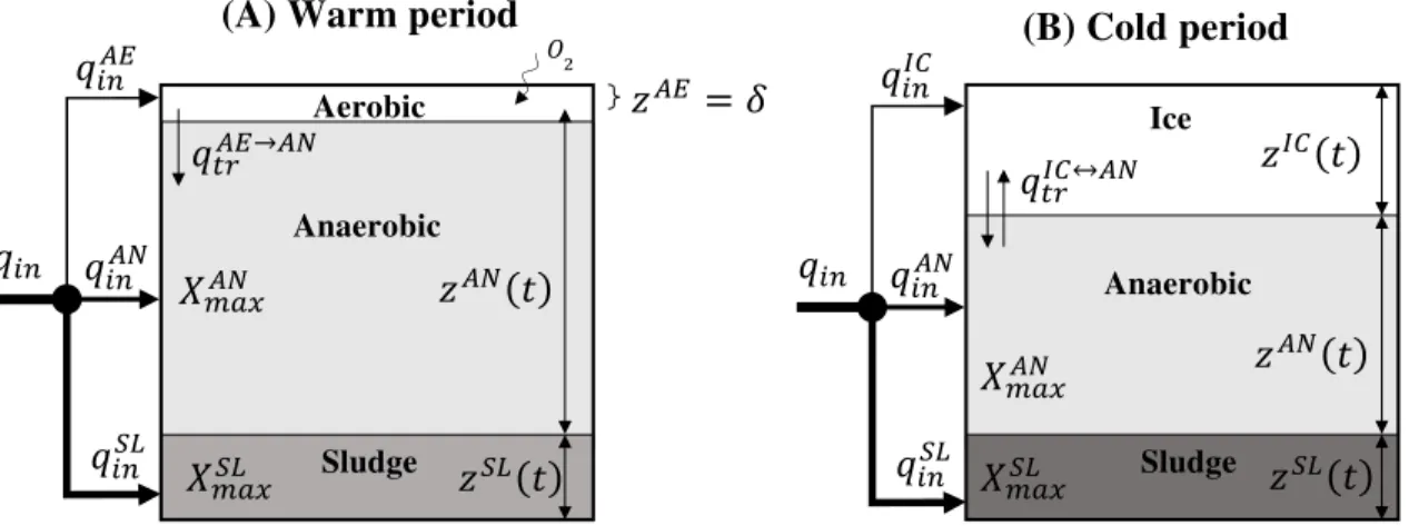
71 72 2. MODEL FORMULATION 73 2.1 Modeling approach 74
The proposed model uses a multi-layer approach to describe the existence of several
75
distinct zones in a facultative lagoon. The multi-layer approach to modeling was successfully
76
applied in the past to various biological systems with significant oxygen, carbon source, or
77
biomass gradients [Rauch et al., 1999; Tartakovsky and Guiot, 1997]. Accordingly, the model
78
assumes the existence of three distinct layers at any given time, each assumed to be completely
79
mixed. In the relatively warm period in the summer, the top layer is assumed to be aerobic liquid,
80
the middle layer anaerobic liquid, and the bottom layer is sludge, assumed to always be under
81
anaerobic conditions. The depth of the aerobic layer is expected to be restricted to 20 – 50 cm
82
due to limited oxygen penetration (no forced aeration) and fast oxygen consumption by aerobic
83
bacteria [Hunik et al., 1994; Stephenson et al., 1999; Tartakovsky et al., 2006].
84
In the cold period the WSP is assumed to be completely ice-capped, which means that
85
there is no oxygen flow from the air into the liquid (the depletion of oxygen in the liquid due to
86
icing is nearly instantaneous). Consequently, there is no aerobic layer during the cold season.
87
The anaerobic layer of liquid can become partially or completely frozen, depending on ambient
88
temperature. The sludge layer is assumed to remain in a liquid state due to its depth as well as
89
due to exothermic microbial activities such as hydrolysis of solids and anaerobic biodegradation
90
of soluble organics, which result in heat production and help to prevent the sludge layer from
91
freezing.
Figure 1 shows a schematic diagram of the layers considered during the warm and cold
93
periods. During the warm season the depth (or thickness) of the aerobic layer (zAE) is considered
94
to be constant, while the depth of the anaerobic (zAN) and the sludge (zSL) layers increases as a
95
result of the daily addition of raw wastewater.
96
2.2 Icecap modeling 97
A separate model was developed to estimate the thickness of ice as a function of the
98
ambient temperature profiles (degree days). This model was developed based on work by Ashton
99
et al [Ashton, 1986; 1989] with modifications to account for the heat flux from the relatively
100
warm sewage inflow to the ice layer and for the insulating properties of snow cover. A detailed
101
description of the icecap model is provided in Supplementary Information (Appendix A). The
102
direct coupling of the icecap model to the multi-layer lagoon model would have resulted in more
103
complex computations and a slower combined model with a marginal improvement in accuracy.
104
Instead, the icecap model is used to estimate the time at which the icecap begins to form, the
105
time at which it reaches maximum thickness, and the time at which it completely melts. The
106
maximum icecap thickness is also estimated. These estimated values are subsequently used in the
107
lagoon model under the simplifying assumption of constant rate of freeze (ice growth) and
108
constant rate of ice thaw.
109
2.3 Biodegradation modeling 110
In formulating the biodegradation, several simplifying assumptions were made towards
111
reducing model integration time and facilitating model calibration. Although ADM1 and ASM3
112
models consider multiple microbial populations, in the absence of Arctic-specific data on the
113
distribution of microbial populations, the proposed model only aerobic heterotrophic (XB,H) and
114
anaerobic (XB,AN) microorganisms. These populations are assumed to be present in all layers.
Also, only readily biodegradable soluble (Ss) and particulate (Xs) organic materials are
116
considered in the material balances, i.e., the current version of the model does not include
117
nitrogen and phosphorus balances.
118
The aerobic and anaerobic liquid layers are assumed to have a saturation (maximal
119
attainable) concentration (Xmax) of suspended solids. At the end of each day of model integration,
120
the solids in excess of this saturation concentration are assumed to settle directly into the sludge
121
layer. Another simplifying assumption is that removal (or settling) of solids from the aerobic and
122
anaerobic layers to the sludge layer is instantaneous. Also, all dissolved components are assumed
123
to be uniformly distributed between the layers (instant mixing assumption). The instantaneous
124
settling and mixing assumptions can be justified by the fact that the lagoon performance is
125
simulated over a period of one year. Therefore the settling and mixing processes occurring at a
126
scale of several hours or even days may be considered instantaneous without any significant loss
127
of accuracy.
128
Material balances and kinetic equations describing the hydrolysis of particulate organic
129
materials and the growth of XB,H and XB,AN microbial populations on soluble organic materials
130
were adapted from ASM3 [Henze et al., 2000]. In particular, multiplicative Monod kinetic
131
equations are used to describe aerobic and anaerobic (anoxic) growth of heterotrophic biomass,
132
which is dependent on readily available dissolved substrate (Ss) and dissolved oxygen (SO)
133 concentrations, i.e. 134 � = � ��, ( �� �, +��) ( � , +� ) � , +� ��, ( �� �, +��) ( , ,+� ) � , , (1) 135
where � is the specific growth rate of the aerobic heterotrophic microorganisms, � ��, is the
136
maximum specific growth rate of the heterotrophs, �, and , are the half saturation
137
constants, and ,� is the inhibition constant.
The specific growth rate of anaerobic microorganisms (��� is described as 139 ��� = � ��,��( �� �, +��) ( , ,+� ) ( , ,+ , ) � ,�� , (2) 140
where � ��,�� is the maximum specific growth rate of the anaerobes, �,�� is the half-saturation
141
constant of anaerobic microorganisms and ��,� is the self-inhibition constant.
142
The rate of hydrolysis of particulate materials plays an important role in determining the
143
outcome of wastewater treatment, as it often represents the slowest biodegradation step. The
144
following expression, adapted from ASM3 model, is used to describe the specific hydrolysis rate
145
ℎ in the proposed model, where both aerobic and anaerobic populations contribute to the
146 hydrolysis: 147 ℎ = ℎ, � , + , ⁄ , + �⁄( , + , ) � , � + � ,�� � , (3) 148
where ℎ, is the maximum hydrolysis rate, , and , are the half saturation constants of
149
hydrolysis and is the fraction of anaerobes(� ,��) contributing to hydrolysis.
150
The rates of aerobic and anaerobic degradation of soluble organic materials are assumed
151
to be proportional to the growth rates of the corresponding microbial populations. A detailed
152
description of these equations and the material balances of the model are provided in
153
Supplementary Information (Appendix B).
154
155
2.4 Numerical methods 156
At each moment in time the performance of the WSP is described by the COD
157
concentration in the lagoon (total - CODt, soluble - CODs and particulate - CODp) calculated as
158 � = �∑ (�� � + � ��)�� � (4) 159
� = �∑ ( � � + ��)�� � (5) 160 � �= � + � (6) 161
where Vt is the combined volume of all layers (volume of the lagoon content), i is the
162
layer index, = � , , � , corresponding to the aerobic, ice, anaerobic, and sludge layers.
163
First-order differential equations, corresponding to the model material balances, are
164
numerically solved using ODE45 function of Matlab R2010 (Mathworks, Natick, MA, USA).
165
Model parameters are estimated using Matlab’s unconstrained optimization function fminsearch,
166
to minimize the root mean squared error (RMSE) between estimated and observed values of
167
total, soluble and particulate COD concentrations:
168
� = √∑ � ∑ (�= , − , ) . (7)
169
Here, is the total number of measurements; represents experimentally measured (or
170
observed) values; represents the corresponding model output (estimated) values; k is the
171
index corresponding to COD components, k = { � �, � , � }.
172
As will be described later, the sensitivity of model results to parameter values was used in
173
the calibration/validation process. The relative sensitivity of each model parameter with
174
respect to each output variable was computed as:
175
=��� ∙� (8)
176
where = { � �, � , � } and j is the parameter’s index.
177
178
3. MODEL CALIBRATION AND VALIDATION 179
The proposed model was calibrated and validated using data collected at three arctic
180
lagoons situated in the hamlets of Pond Inlet, Gjoa Haven, and Kugaruuk (Nunavut, Canada).
The three are engineered lagoons, with surface areas (when full) of about 40,000, 20,000, 13,000
182
m2, and average depths (when full) of about 1.6, 3 and 3 m, respectively.
183
Available measurements at these lagoons included characterization of raw sewage and
184
samples withdrawn from the lagoons (typically near the discharge point) during one year. Only
185
two to three sampling campaigns per year were carried out at each location, typically in early or
186
mid-summer as well as late-summer or early fall, towards decanting. Information provided
187
through these campaigns in include total and soluble COD and/or BOD concentration, and total
188
suspended solid (TSS) concentration. If total COD concentration values were unavailable, they
189
were estimated using BOD5 measurements by assuming a COD to BOD5 ratio of 2 (i.e., 1 mg L-1
190
of BOD5 is equivalent to 2 mg L-1 of COD). Pond Inlet lagoon characterization results were
191
taken from [Ragush et al., 2015], while measurements at Gjoa Haven, and Kugaruuk were
192
provided by Environment Canada (unpublished data corresponding to lagoon characterization
193
from September 2009 to September 2010). Also, daily temperatures, precipitation (rain and
194
snow) and depth of snow on the ground at each location were obtained from the publicly
195
available Environment Canada website for the corresponding years and used for icecap
196
formation/melting dates and thickness computations.
197
198
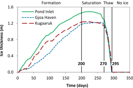
3.1 Icecap formation 199
The icecap formation and decay model described in Appendix A was used to estimate the
200
beginning and end of ice formation as well as the icecap thickness. Figure 2 shows the resulting
201
ice thickness profiles calculated for the Pond Inlet, Gjoa Haven, and Kugaruuk lagoons in
202
Nunavut, Canada, based on the temperature profiles from September 2009 to September 2010. In
203
the fall of 2009 icecap started forming around September 15th to September 20th (relatively soon
after decant) in all three locations. Consequently, September 15th was considered as t = 0 (see
205
Figure 2) for the model calibration calculations. The calculations of ice thickness were carried
206
out for 350 days. Water discharge was assumed to take place between days 350 – 365 (not shown
207
in Figure 2) and effective average snow cover thickness was assumed to be 50% of the “snow on
208
the ground” values provided by Environment Canada data.
209
As can be seen from Figure 2, at all three locations a near constant ice formation rate is
210
estimated, resulting in a linear increase of ice thickness up to about day 200. Subsequently, a
211
constant ice thickness is estimated between days 200-270, followed by a period of relatively fast
212
thaw that culminates with ice-free surface at about day 295. It should be noted that only 50% of
213
the accumulated snow on the ground (as recorded by Environment-Canada) was effectively
214
considered for heat-flux calculations, as a portion of the snow was assumed to have been blown
215
away due to winds.
216
As mentioned earlier, the ice-formation model was not directly coupled with the lagoon
217
model. Rather, these simulation results were used to determine ice formation parameters (start of
218
ice formation and thaw as well as constant ice formation and thaw rates), which were used as
219
inputs for the multi-layer lagoon model.
220
221
3.2 Biodegradation kinetics 222
Initially, model parameters related to aerobic heterotrophic activity were taken from ASM3
223
[Henze et al., 2000], while degradation rates under anaerobic conditions were assumed from
224
[Lettinga et al., 2001]. Also, initial value of the oxygen transfer coefficient (kL) was adapted
225
from the work of Chaturvedi et al. [Chaturvedi et al., 2014], assuming wind speeds between 1
226
and 8 m s-1 and an average water temperature of 10 ºC. Table 1 provides the values of all model
parameters and Tables 2 and 3 describe influent wastewater composition and initial conditions
228
used for model integration.
229
Considering the rather large number of model parameters and the limited number of available
230
measurements (only 2-3 sets of COD and TSS measurements were available for each lagoon,
231
with no biomass measurements at all), it was deemed best to identify a small subset of model
232
parameters with the largest influence on model outputs and subsequently calibrate the model
233
using only this limited subset, while all other parameters are kept constant at values obtained
234
from the literature. The most influential parameters were identified through a sensitivity analysis,
235
using Eq. 8. Table 4 summarizes results of this sensitivity analysis. Based on these results, a
236
subset of three parameters was selected for estimation, namely the maximum specific growth rate
237
of anaerobic microorganisms (� ��,��), the rate of solid organic matter hydrolysis ( ℎ), and the
238
oxygen transfer coefficient (kL).
239
Parameter estimation (model calibration) was performed using data of two lagoons, Pond
240
Inlet and Gjoa Haven, whereby values of parameters � ��,� , ℎ, and kL that minimized RMSE
241
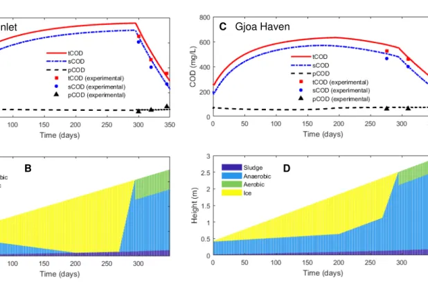
(Eq. 7) were identified (all other parameters were held constant). Figure 3 provides the resulting
242
profiles of total, soluble, and particulate CODs for the Pond Inlet and Gjoa Haven lagoons with
243
the calibrated parameters. Table 5 summarizes the estimated values of these parameters. The
244
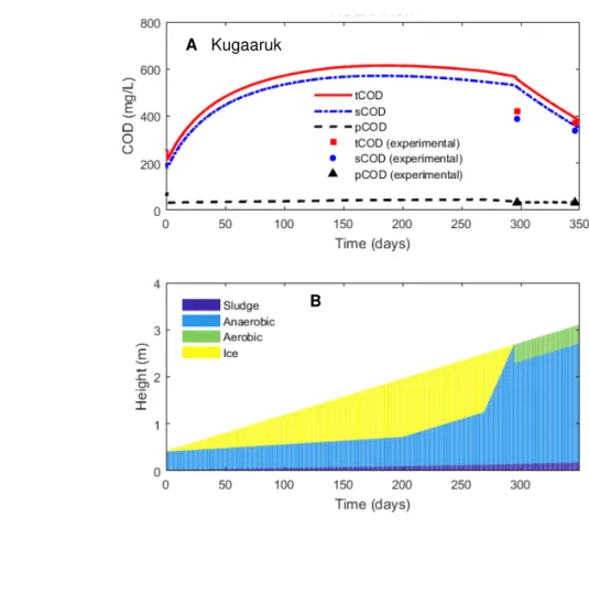
model was subsequently validated by applying the estimated parameter values to the Kugaruuk
245
lagoon. Figure 4 illustrates a comparison between estimated and observed values of COD and
246
TSS measurements in the Kugaaruk lagoon.
247
It can be seen that in all cases the model predicted a COD accumulation during winter
248
months followed by a relatively fast COD degradation during the ice-free period. While the
249
predicted trends qualitatively agreed with the observed values, the RMSE value for Kugaruuk
validation was higher (as expected) than for the lagoons used for parameter estimation (Table 5).
251
It was nonetheless deemed that the model showed a reasonable capability to correctly predict the
252
measured trends in total and dissolved COD concentrations.
253
As mentioned earlier, the small number of measured data available for calibration
254
presented a significant challenge to the confidence with which the results could be evaluated.
255
Consequently, an additional calibration method was undertaken whereby the estimation
256
procedure was repeated for each lagoon individually. In this case however, the oxygen transfer
257
coefficient was kept at the estimated value of 6.4 m d-1 , while � ��,� and ℎ, values were
re-258
estimated for each lagoon. As shown in Table 5, this approach resulted in smaller RMSE values
259
and also demonstrated the differences between the lagoons in terms of � ��,� and ℎ, values.
260
Since parameter sensitivity analysis showed high impact of these parameters on the model
261
outputs, the differences between the lagoons are likely represented by the differences between
262 lagoon-specific values. 263 264 4. DISCUSSION 265
While the dearth of calibration data limits the confidence in the accuracy of the results,
266
some important, and not altogether expected, trends on the performance of facultative sewage
267
lagoons in the Arctic can be discerned from the model outputs. For example, a clear trend
268
emerges, whereby soluble COD concentration increases consistently during winter months
269
(Figures 3, 4). This can be explained by the fact that during winter, particulate COD settles and
270
continuously undergoes hydrolysis in the sludge layer of the lagoon, albeit at a low rate, while at
271
the same time a relatively slow anaerobic degradation acts to reduce soluble COD concentration.
272
When the icecap melts away, fast reduction in soluble COD concentration can be observed, as
aerobic activity initiates and increases in the top layer. The aerobic growth of suspended
274
heterotrophic biomass is accompanied by biomass settling, since the suspended biomass
275
concentration in the aerobic layer is limited by the maximum attainable density (Xmax). The
276
aerobic biomass in the sludge layer contributes to hydrolysis of solids according to Eq. (3).
277
Notably, the hydrolysis rate is not limited by the absence of oxygen in the sludge. As a result,
278
the overall rate of hydrolysis accelerates during summer.
279
Another important observation can be made that although the degradation of organic
280
materials under anaerobic conditions is slow (compared to aerobic degradation), the anaerobic
281
activity provides a significant contribution to the overall COD removal in the lagoon due to the
282
fact that this activity takes place throughout the year and also due to the high sludge density. This
283
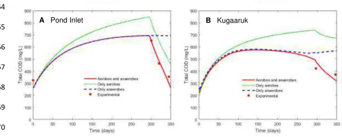
can be further demonstrated by comparing different scenarios of COD degradation in the shallow
284
Pond Inlet lagoon (Figure 5A) and the deep Kugaruuk lagoon (Figure 5B). In one scenario the
285
COD degradation is simulated with the anaerobic rate of COD degradation set to zero (only
286
aerobes), while in the other scenario the aerobic degradation rate is set to zero (only anaerobes).
287
It is clear that the absence of anaerobic biodegradation throughout the winter results in COD
288
accumulation in both lagoons. If zero anaerobic activity is assumed, the rate of aerobic
289
degradation required to achieve observed COD concentrations at the end of summer would have
290
to be increased to an unrealistically high value of approximately 10 d-1, which is not likely given
291
that water temperature in the lagoons does not typically exceed 10-12oC during the summer.
292
Clearly, only a combination of both aerobic and anaerobic degradation activities results in the
293
COD profiles matching the field measurements.
294
Interestingly, the model predicts different COD profiles during winter for each lagoon.
295
Pond Inlet lagoon is relatively shallow (about 1.6 m average depth when full), in which the ice
thickness can reach a maximum of about 1.4 m (Figure 2). This results in an expected gradual
297
increase of total and soluble COD concentrations throughout the winter due to the absence of
298
biological activity in the ice layer. Although, anaerobic degradation continues in the sludge layer,
299
it is not sufficient to considerably reduce soluble CODs (Figure 3). This prediction agrees well
300
with the high COD value measured at the beginning of summer, right after the complete melting
301
of the ice cover. This accumulation of CODs is followed by a relatively fast COD reduction in
302
the summer. It can be seen that even in the shallow Pond Inlet lagoon anaerobic degradation
303
contributes to the overall COD removal as the comparison of different scenarios shown in Figure
304
5A indicates.
305
The predicted COD profiles in the much deeper Gjoa Haven, and Kugaruuk lagoons followed
306
a somewhat different pattern. In these lagoons a fast increase in COD concentrations is predicted
307
during the first 50-60 days, followed by slow COD concentration decrease throughout the winter,
308
due to anaerobic activity in the unfrozen anaerobic and sludge layers under the ice. The rate of
309
COD degradation is predicted to accelerate during the summer (Figures 3 and 4) due to aerobic
310
activity. It is noted (again) that only COD trends in the summer months can be confirmed by
311
observed data. Profiles of particulate CODs in all lagoons were similar with a somewhat higher
312
concentration during summer. Fast growth of aerobic bacteria in the upper oxygenated layer
313
during summer months results is accompanied by biomass settling, which contributes to
314
particulate CODs as well as to sludge accumulation, although it increases the rate of hydrolysis
315
according to model equation (3). Notably, solids hydrolysis does not require dissolved oxygen
316
and therefore proceeds in the sludge layer, where the biomass concentration is the highest.
317
A detailed look at the model outputs and the parameter estimation results suggests that
318
the difference in COD profiles can be explained by the differences in lagoon depths. The shallow
Pond Inlet lagoon is frozen during 260 days of the year (most of this period frozen through,
320
except the sludge layer), which significantly limits anaerobic activity during winter months.
321
During the summer months a high degradation rate is achieved due to higher ratio of aerobic to
322
anaerobic activity. In Pond Inlet, an aerobic layer thickness of 40 cm corresponds to
323
approximately 25% of this lagoon depth, while in two other lagoons the aerobic layer comprises
324
less than 15% of the total lagoon depth. Consequently, aerobic degradation provides a relatively
325
higher contribution to COD removal at the Pond Inlet lagoon compared to two other, deeper
326
lagoons (Figure 5).
327
Gradual degradation of COD throughout winter in the Gjoa Haven and Kugaruuk lagoons
328
is attributed to the existence of a liquid anaerobic layer throughout the winter months (Figures 3,
329
4), which supports anaerobic activity. As a result, a moderate COD concentration decrease is
330
predicted, despite the presence of the icecap.
331
The importance of considering anaerobic microbial activity in northern lagoons appears
332
to be an immediate conclusion, with important implications for future lagoon design. It can be
333
surmised that some combination of deep and shallow lagoons is likely to provide the best results
334
in terms of degradation of organics in the sewage. In fact, there is some evidence that multi-cell
335
lagoons in the Arctic are functioning well. It appears that a deep first lagoon is likely to provide
336
substantial anaerobic degradation in winter, while a shallow and wide second lagoon will provide
337
substantial aerobic degradation in summer.
338
Another important consideration in evaluating Arctic lagoon performance could be
339
related to the contribution of algae blooms to COD removal. While the current version of the
340
model does not consider algae growth, it appears to be indirectly accounted for by the oxygen
341
transfer coefficient (kL). During long summer days algae are expected to supply oxygen to the
top (aerobic) layer of the lagoon. Indeed, parameter estimation yielded a kL value of 6.4, which is
343
somewhat higher than a range of values suggested in literature (0.9 – 6.0 m d-1), as indicated in
344
Table 1. In addition to increased oxygen supply, both phototrophic and heterotrophic growth of
345
algae are likely to contribute to solids accumulation, especially after the end of summer, when
346
temperatures become lower and days become shorter, before the formation of icecap. Future
347
version of the Arctic lagoon model needs to be extended to account for this phenomenon as well
348
as for nitrogen and phosphorus removal at low temperatures.
349
350
5. CONCLUSION 351
This study describes a mathematical model capable of simulating the biodegradation of
352
wastewater in arctic WSPs. The model accounts for several unique features of Arctic lagoons,
353
including the periodic nature of lagoon operation and the existence of icecap for most of the
354
lagoon operation cycle. The proposed model is calibrated and validated using limited observed
355
data, obtained at three arctic lagoons. Acceptable agreement between the predicted and measured
356
COD and TSS concentration profiles was obtained. Analysis of predicted COD concentration
357
profiles suggests significant anaerobic biodegradation of organic materials throughout winter
358
months. The model can be used for analyzing and improving Arctic lagoon design.
359
360
Acknowledgement 361
The authors wish to acknowledge Environment and Climate Change Canada (ECCC) and in
362
particular Ms. Shirley Anne Smyth, who provided unpublished data that were invaluable for the
363
initial calibration of the model. Also Mr. Babesh Roy of the Government of Nunavut, who
364
facilitated data sharing on the Pond Inlet lagoon.
Notations 366
� Lagoon’s surface, m2
Specific interfacial area, m-1 BOD Biological oxygen demand, mg L-1
�� Decay rate of � ,��*, d-1
Decay rate of � , *, d-1
COD Chemical oxygen demand, mg L-1
CSTR Continuous stirred tank reactor Fraction of � yielding ��, %
ℎ Lagoon’s depth, m
��,� Self-inhibition coefficient for � ,��, mg L-1 � Oxygen mass transfer coefficient**, m d-1
, Half-saturation coefficient of for � , , mg L-1 ,� Inhibition coefficient of for � , , mg L-1 �,�� Half-saturation coefficient of � for � ,��, mg L-1 �, Half-saturation coefficient of � for � , , mg L-1
, Half-saturation coefficient of �� for � , , mg L-1 ℎ Maximum specific hydrolysis rate*, d-1
MSE Mean squared error
�� Input flow rate, L d-1
����→ Transfer flow rate from layer to layer , L d-1 Concentration of soluble oxygen, mg L-1
, �� Maximum value for , mg L-1
� Concentration of soluble inert materials, mg L-1
Concentration of biodegradable soluble substrate, mg L-1 �� ���� Start of ice formation, d
���� End of ice thaw, d
� Lagoon’s volume, L
� ,�� Concentration of heterotrophic bacteria, mg L-1
� , Concentration of anaerobic bacteria, mg L-1
�� Concentration of particulate inerts, mg L-1
���,���� Solids saturation density in liquid, mg L-1
���� Solids saturation density in sludge, mg L-1
����� Solids saturation density in ice, mg L-1
�� Concentration of biodegradable particulate substrate, mg L-1 �, Yield factor of � for � , mg/mg
�,�� Yield factor of � for � ,��mg/mg
, Yield factor of for � , , mg/mg
� layer height, m
����� Maximum thickness aerobic layer, m
����� Maximum thickness of ice layer, m
� Solids settling, %
��� Period of ice formation/thaw, d
ℎ Correction factor for hydrolysis by � ,��*
� Correction factor anoxic growth � ,
� ��, Maximum specific growth rate of � , *, d-1
� ��,�� Maximum specific growth rate of � ,��*, d-1 Indices
� Aerobic layer
� Anaerobic layer
Final
Experimental values
Heterotrophic microbial population
ℎ Related to hydrolysis
Inert Ice layer
Influent Initial Maximum
� Oxygen, , mg L-1
Sludge layer or related to the soluble substrate Simulated values
� Transfer between layers
367
368
REFERENCES 370
Aldana, G. J., B. J. Lloyd, K. Guganesharajah, and N. Bracho (2005), The development and
371
calibration of a physical model to assist in optimising the hydraulic performance and design of
372
maturation ponds, Water Sci. Technol., 51(12), 173-181.
373
Ashton, G. D. (1983), Predicting Lake Ice Decay, Cold regions research and engineering lab
374
Hanover NH.
375
Ashton, G. D. (1986), River and lake ice engineering, Water Resources Publication.
376
Ashton, G. D. (1989), Thin ice growth, Water Resour. Res., 25(3), 564-566.
377
Banks, C. J., G. B. Koloskov, A. C. Lock, and S. Heaven (2003), A computer simulation of the
378
oxygen balance in a cold climate winter storage WSP during the critical spring warm-up period,
379
Water Sci. Technol., 48(2), 189-196. 380
Batstone, D. J., J. Keller, I. Angelidaki, S. V. Kalyuzhnyi, S. G. Pavlostathis, A. Rozzi, W. T. M.
381
Sanders, H. Siegrist, and V. A. Vavilin (2002), The IWA anaerobic digestion model no 1
382
(ADM1), Water Sci. Technol., 45(10), 65-73.
383
Beran, B., and F. Kargi (2005), A dynamic mathematical model for wastewater stabilization
384
ponds, Ecol. Model., 181(1), 39-57.
385
Borja, R., E. González, F. Raposo, F. Millán, and A. Martín (2002), Kinetic analysis of the
386
psychrophilic anaerobic digestion of wastewater derived from the production of proteins from
387
extracted sunflower flour, J. Agric. Food Chem., 50(16), 4628-4633.
388
Chaturvedi, M. K. M., S. D. Langote, D. Kumar, and S. R. Asolekar (2014), Significance and
389
estimation of oxygen mass transfer coefficient in simulated waste stabilization pond, Ecol. Eng.,
390
73, 331-334. 391
Chen, Y. R., and A. G. Hashimoto (1978), Kinetics of methane fermentation, paper presented at
392
Biotechnol. Bioeng. Symp.
393
Dochain, D., S. Gregoire, A. Pauss, and M. Schaegger (2003), Dynamical modelling of a waste
394
stabilisation pond, Bioprocess. Biosyst. Eng., 26(1), 19-26.
395
Gu, R., and H. G. Stefan (1995), Stratification dynamics in wastewater stabilization ponds,
396
Water Res., 29(8), 1909-1923. 397
Henze, M., W. Gujer, T. Mino, and M. C. M. van Loosdrecht (2000), Activated sludge models
398
ASM1, ASM2, ASM2d and ASM3, IWA publishing. 399
Houweling, C. D., L. Kharoune, A. Escalas, and Y. Comeau (2005), Modeling ammonia removal
400
in aerated facultative lagoons, Water Sci. Technol., 51(12), 139-142.
401
Hunik, J. H., C. G. Bos, M. P. Hoogen, C. D. DeGooijer, and J. Tramper (1994),
Co-402
immobilized Nitrosomonas europea and Nitrobacter agilis cells: validation of a dynamic model
403
for simultaneous substrate conversion and growth in k-carrageenan gel beads, Biotechnol.
404
Bioeng., 43, 1153-1163. 405
Jupsin, H., and J. L. Vasel (2007), Modelisation of the contribution of sediments in the treatment
406
process case of aerated lagoons, Water Sci. Technol., 55(11), 21-27.
407
Kayombo, S., T. S. A. Mbwette, A. W. Mayo, J. H. Y. Katima, and S. E. Jorgensen (2000),
408
Modelling diurnal variation of dissolved oxygen in waste stabilization ponds, Ecol. Model.,
409
127(1), 21-31. 410
Langergraber, G., D. P. L. Rousseau, J. García, and J. Mena (2009), CWM1: a general model to
411
describe biokinetic processes in subsurface flow constructed wetlands, Water Sci. Technol.,
412
59(9), 1687-1697. 413
Lettinga, G., S. Rebac, and G. Zeeman (2001), Challenge of psychrophilic anaerobic wastewater
414
treatment, Trends Biotechnol., 19(9), 363-370.
415
Martínez, F. C., A. T. Cansino, M. A. A. García, V. Kalashnikov, and R. L. Rojas (2014),
416
Mathematical analysis for the optimization of a design in a facultative pond: indicator organism
417
and organic matter, Math. Probl. Eng., 2014.
418
Peng, J. F., B. Z. Wang, Y. H. Song, and P. Yuan (2007), Modeling N transformation and
419
removal in a duckweed pond: model development and calibration, Ecol. Model., 206(1),
147-420
152.
421
Perry, R., and D. Green (1984), Perry's Chemical Engineers' Handbook, McGraw-HiII, Inc.
422
NewYork.
423
Ragush, C. M., J. J. Schmidt, W. H. Krkosek, G. A. Gagnon, L. Truelstrup-Hansen, and R. C.
424
Jamieson (2015), Performance of municipal waste stabilization ponds in the Canadian Arctic
425
Ecological Eng., 83, 413-421. 426
Rauch, W., H. Vanhooken, and P. A. Vanrolleghem (1999), A simplified mixed-culture biofilm
427
model, Wat. Res., 33, 2148-2162.
428
Sah, L., D. P. L. Rousseau, and C. M. Hooijmans (2012), Numerical modelling of waste
429
stabilization ponds: where do we stand?, Water Air Soil Pollut., 223(6), 3155-3171.
430
Sah, L., D. P. L. Rousseau, C. M. Hooijmans, and P. N. L. Lens (2011), 3D model for a
431
secondary facultative pond, Ecol. Model., 222(9), 1592-1603.
432
Salter, H. E., C. T. Ta, S. K. Ouki, and S. C. Williams (2000), Three-dimensional computational
433
fluid dynamic modelling of a facultative lagoon, Water Sci. Technol., 42(10-11), 335-342.
434
Stephenson, R. J., A. Patoine, and S. R. Guiot (1999), Effects of oxygenation and upflow liquid
435
velocity on a coupled anaerobic/aerobic reactor system, Wat. Res., 33, 2855-2863.
Sweeney, D. G., J. B. Nixon, N. J. Cromar, and H. J. Fallowfield (2005), Profiling and modelling
437
of thermal changes in a large waste stabilisation pond, Water Sci. Technol., 51(12), 163-172.
438
Sweeney, D. G., N. J. Cromar, J. B. Nixon, C. T. Ta, and H. J. Fallowfield (2003), The spatial
439
significance of water quality indicators in waste stabilization ponds-limitations of residence time
440
distribution analysis in predicting treatment efficiency, Water Sci. Technol., 48(2), 211-218.
441
Tartakovsky, B., and S. R. Guiot (1997), Modeling and analysis of layered stationary anaerobic
442
granular biofilms, Biotechnol. Bioeng., 54, 122-130.
443
Tartakovsky, B., M. F. Manuel, and S. R. Guiot (2006), Degradation of trichloroethylene in a
444
coupled anaerobic-aerobic bioreactor : modeling and experiment, Biochemical Engineering
445
Journal, 26(1), 72-81. 446
Toprak, H. (1994), Empirical modelling of sedimentation which occurs in anaerobic waste
447
stabilization ponds using a lab‐scale semi‐continuous reactor, Environ. Technol., 15(2), 125-134.
448
van der Berg, L. (1977), Effect of temperature on growth and activity of a methanogenic culture
449
utilising acetate, Can. J. Microbiol., 23(7), 898-902.
450 451 452 453 454 455 456 457
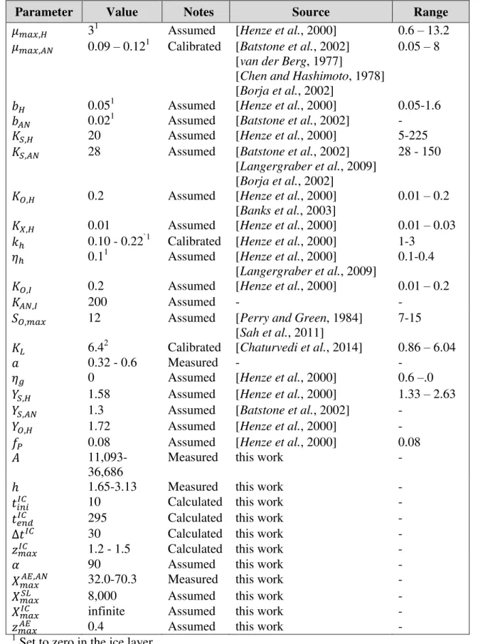
Table 1. Values of the lagoon model parameters.
458
Parameter Value Notes Source Range
� ��, 31 Assumed [Henze et al., 2000] 0.6 – 13.2
� ��,�� 0.09 – 0.121 Calibrated [Batstone et al., 2002]
[van der Berg, 1977]
[Chen and Hashimoto, 1978] [Borja et al., 2002]
0.05 – 8
0.051 Assumed [Henze et al., 2000] 0.05-1.6
�� 0.021 Assumed [Batstone et al., 2002] -
�, 20 Assumed [Henze et al., 2000] 5-225
�,�� 28 Assumed [Batstone et al., 2002]
[Langergraber et al., 2009] [Borja et al., 2002]
28 - 150
, 0.2 Assumed [Henze et al., 2000]
[Banks et al., 2003]
0.01 – 0.2
, 0.01 Assumed [Henze et al., 2000] 0.01 – 0.03
ℎ 0.10 - 0.22`1 Calibrated [Henze et al., 2000] 1-3
ℎ 0.11 Assumed [Henze et al., 2000]
[Langergraber et al., 2009]
0.1-0.4
,� 0.2 Assumed [Henze et al., 2000] 0.01 – 0.2
��,� 200 Assumed - -
, �� 12 Assumed [Perry and Green, 1984]
[Sah et al., 2011]
7-15
� 6.42 Calibrated [Chaturvedi et al., 2014] 0.86 – 6.04
0.32 - 0.6 Measured - -
� 0 Assumed [Henze et al., 2000] 0.6 –.0
�, 1.58 Assumed [Henze et al., 2000] 1.33 – 2.63
�,�� 1.3 Assumed [Batstone et al., 2002] -
, 1.72 Assumed [Henze et al., 2000] -
0.08 Assumed [Henze et al., 2000] 0.08
�
11,093-36,686
Measured this work -
ℎ 1.65-3.13 Measured this work -
�� ��� 10 Calculated this work -
��� 295 Calculated this work -
��� 30 Calculated this work -
����� 1.2 - 1.5 Calculated this work -
� 90 Assumed this work -
���,���� 32.0-70.3 Measured this work -
����� 8,000 Assumed this work -
����� infinite Assumed this work -
����� 0.4 Assumed this work -
1
Set to zero in the ice layer
459
2
Only considered for the aerobic layer
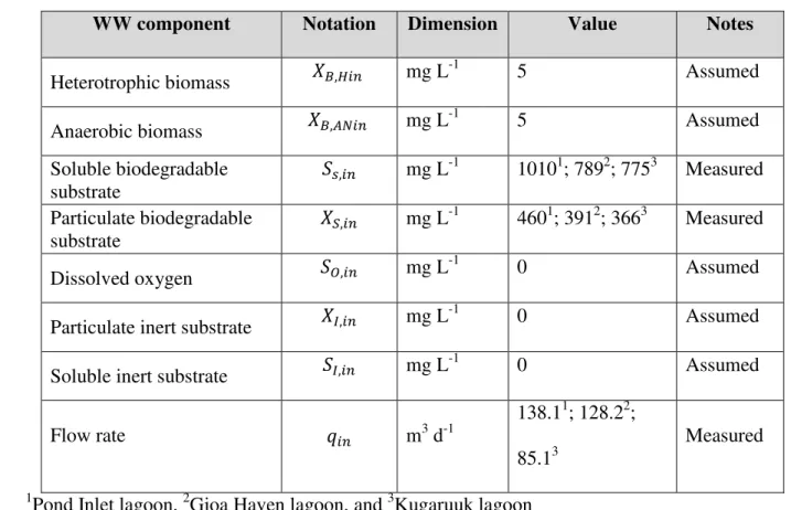
Table 2. Influent wastewater composition.
461
WW component Notation Dimension Value Notes
Heterotrophic biomass � , � mg L -1 5 Assumed Anaerobic biomass � ,��� mg L -1 5 Assumed Soluble biodegradable substrate ,� mg L-1 10101; 7892; 7753 Measured Particulate biodegradable substrate ��,� mg L-1 4601; 3912; 3663 Measured Dissolved oxygen ,� mg L -1 0 Assumed
Particulate inert substrate ��,� mg L
-1
0 Assumed
Soluble inert substrate �,� mg L
-1 0 Assumed Flow rate �� m3 d-1 138.11; 128.22; 85.13 Measured 1
Pond Inlet lagoon, 2Gjoa Haven lagoon, and 3Kugaruuk lagoon
462
Table 3. Initial conditions used for lagoon model integration.
464
Parameter Dimension
Layer
Notes Aerobic Anaerobic Sludge Ice
� , mg L-1 10 0 0 0 Assumed � ,�� mg L-1 0 10 100 0 Assumed mg L-1 2601; 2002,3 2601; 2002,3 2601; 2002,3 0 Measured1 Assumed2,3 �� mg L-1 641; 502,3 641; 502,3 ����� 0 Measured1 Assumed2,3 mg L-1 3.5 0 0 0 Measured �� mg L-1 0 0 0 0 Assumed � mg L-1 0 0 0 0 Assumed � m ����� 0 0.02 0 Assumed 465 1
Pond Inlet lagoon, 2Gjoa Haven lagoon, and 3Kugaruuk lagoon
466 467 468
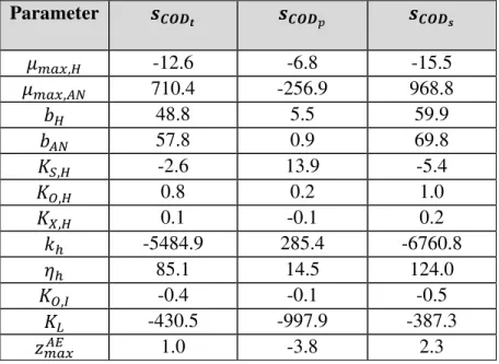
Table 4. Parameter sensitivity values with respect to CODt, CODp, and CODs variations. 469 470 Parameter � � ��, -12.6 -6.8 -15.5 � ��,�� 710.4 -256.9 968.8 48.8 5.5 59.9 �� 57.8 0.9 69.8 �, -2.6 13.9 -5.4 , 0.8 0.2 1.0 , 0.1 -0.1 0.2 ℎ -5484.9 285.4 -6760.8 ℎ 85.1 14.5 124.0 ,� -0.4 -0.1 -0.5 � -430.5 -997.9 -387.3 ����� 1.0 -3.8 2.3 471 472
473
Table 5. Model calibration and validation results. Notations: PI – Pond Inlet lagoon, GH - Gjoa
474
Haven, and KU – Kugaruuk.
475
476
Lagoon KL kh μmax,AN RMSE Notes
PI and GH 6.40 0.043 0.07 197 calibration KU 6.40 0.043 0.07 195 validation PI 6.40 0.100 0.11 63 re-calibration GH 6.40 0.220 0.09 69 re-calibration KU 6.40 0.22 0.12 102 re-calibration 477 478 479 480 481 482 483
484 485 486 487 488 489 490 491 492 493 494 495 496 497 498
Figure 1. Schematic diagram of the layers considered in the model during (A) warm and (B)
499
cold periods.
500
���= � �
(A) Warm period Aerobic Anaerobic Sludge �� ���� ���� ���� �����→�� ����� ����� ��� � ��� � �� ���� ���� ���� (B) Cold period Ice Anaerobic Sludge ��� � ����� ����� ��� � ��� � �����↔��
501 502 503 504 505 506 507 508 509 510 511 512
Figure 2. Icecap profile simulated using temperature data collected in 2010. Ice thickness values
513
are presented from September 15th 2009 (day 0) until August 31st ,2010 (day 350).
514 515 516 0.0 0.4 0.8 1.2 1.6 0 50 100 150 200 250 300 350 Ice t h ic kn e ss (m ) Time (days) Pond Inlet Gjoa Haven Kugaaruk No ice Thaw Saturation Formation 200 270 295
517 518 519 520 521 522 523 524 525 526 527 528 529 530 531 532 533 534 535
Figure 3. Model calibration results showing a comparison of model outputs with experimental
536
data and predicted layer thickness for (A, B) Pond Inlet and (C, D) Gjoa Haven lagoons.
537 538 B A Pond Inlet D C Gjoa Haven
539 540 541 542 543 544 545 546 547 548 549 550 551 552 553 554 555 556
Figure 4. Model validation results showing a comparison of model outputs with experimental
557
data (A) and predicted layer thickness (B) for Kugaruuk lagoon.
558 559 560 561 B A Kugaaruk
562 563 564 565 566 567 568 569 570 571 572 573 574 575 576 577 578 579 580
Figure 5. A comparison of COD concentration profiles calculated with and without contribution
581
of aerobic and anaerobic degradation for the Pond Inlet (A) and Kugaaruk (B) lagoons.
582
583
SUPPLEMENTARY INFORMATION 584
APPENDIX A. Modelling icecap formation and decay 585
The following equation was used to describe ice formation. This equation is based on
586
work by Ashton [Ashton, 1986; 1989] with modifications to account for the heat flux from the
587
relatively warm sewage inflow to the ice layer and for the insulating properties of snow cover:
588 ∆ℎ = (∆�) [ ℎ − � � �+ ℎ + � − � − ] (A1) where 589
Δh = incremental growth of ice layer thickness [m] over time-step Δt 590
ki = thermal conductivity of ice [W m-1oC-1] (taken as 2.3 (corresponding to temp. of
591
about -10 oC) for this research)
592
ks = thermal conductivity of snow [W m-1oC-1] (taken as 0.4 for this research)
593
Tm = temperature at the ice water interface (assumed 0oC)
594
Tw = temperature of the water under the ice
595
Ta = temperature of air above the ice [oC]
596
Ha = thermal resistance (or heat transfer coefficient) between the uppermost surface and
597
the air above it (i.e., when hs = 0 then Ha = Hia; and when hs > 0 then Ha = Has)
598
Hia = bulk heat transfer coefficient between the top surface temperature of the ice and the
599
air temperature above the ice (taken as 25 [W m-2oC-1] for this research
600
Hsa = bulk heat transfer coefficient between the top surface temperature of snow and the
601
air temperature above the snow (taken as 15 [W m-2oC-1] for this research)
602
Hwi = bulk heat transfer coefficient between the water and the ice (taken as 2.19 [W m-2
603
o
C-1] for this research
ρ = ice density [kg/m-3
] (taken as 919 (corresponding to temp. of about -10 oC) for this
605
research)
606
L = heat of fusion [J/kg-1] (taken as 3.3355•105 for this research)
607
hi = thickness of the ice cover at time-step Δt
608
hs = thickness of the snow cover at time-step Δt
609
When Δt is taken as one day (or 86,400 seconds) the ice layer thickness becomes a
610
function of freezing degree-days.
611
The following equation was used to model the decay of ice over a sewage lagoon. This
612
equation is also based on work by Ashton [Ashton, 1983] with modifications to account for the
613
heat flux from the relatively warm sewage inflow to the ice layer:
614
∆ℎ = (∆�) [− �� − � − � − ] (A2)
Here too, when Δt is taken as one day the ice layer thickness becomes a function of
615
melting degree-days. In the absence of real field data, the water temperature Tw is assumed to
616
have a sinusoidal form over the year with an amplitude of ATw and a period of 365 days. The
617
average temperature in day d is therefore estimated as:
618
= + . � [ + ] = , , … (A3)
where d =1 is the day at which decanting ends. Minimum water temperature was assumed
619
to be 3oC. The amplitude can be expected to be in the range of 4 to 12 degrees.
620
621
APPENDIX B. Biodegradation model 623
The following material balance equations are used to describe sewage biodegradation. The
624
balances are composed for each layer I, where , = � , � , , and j ≠ i.
625 1. Heterotrophic biomass (��, ) 626 ��, � = � ��, � � �, + �� � , + � � , � ⏟
Aerobic growth of heterotrophic biomass
+ �� ��, � � �, + �� ,� ,�+ � � , � ⏟
Anoxic growth of heterotrophic biomass
− ⏟ ��, Decay of heterotrophic biomass +�⏟ ���� (� , � − ��, ) Flow in +��� →� �� (� , − ��, ) ⏟ Transport term 2. Anaerobic biomass (��, ) 627 ��,�� � = � ��,�� � � �,��+ �� ,� ,�+ � ��,� ��,�+ ��,�� � ,�� � ⏟
Growth of anaerobic biomas
− ⏟ ����,�� Decay of anaerobic biomass +�⏟ ���� (� ,��,� − ��,��) Flow in +��� →� �� (� ,��− ��,��) ⏟ Transport term
3. Readily biodegradable soluble substrate (��) 628 � � = − �, � ��, � � �, + �� � , + � � , � ⏟
Aerobic growth of heterotrophic biomass
− � �, � ��, � � �, + �� ,� ,�+ � � , � ⏟
Anoxic growth of heterotrophic biomass
− �,��� ��,�� � � �,��+ �� ,� ,�+ � ��,� ��,�+ ��,�� � ,�� � ⏟
Growth of anaerobic biomas
+ ℎ, �� � (� , � + � ,�� � ) ⁄ , + ���⁄(��, + ��,��) � , � + � ,�� � ⏟ Hy ly i a a i la a i +�⏟ ���� ( ,� − �) Flow in +��� →� �� ( − �) ⏟ Transport term
4. Slowly biodegradable particulate substrate (���) 629 ��� � =⏟ −Decay of ��, heterotrophic biomass +⏟ − ����,�� Decay of anaerobic biomass +��� �� (��,� − ���) +��� →� �� (� − ��) ⏟ Transfer flow ⏟ Flow in − ℎ, �� � (� , � + � ,�� � ) ⁄ , + ���⁄(��, + ��,��) � , � + � ,�� � ⏟ Hy ly i a a i la a i 5. Soluble oxygen (��) 630 � � = − , � ��, � � �, + �� � , + � � , � ⏟
Consumption by aerobic growth of heterotrophic biomass
+⏟ � ( , ��− �) Transfer term +�⏟ ���� ( ,� − �) Flow in +��� →� �� ( − �) ⏟ Transfer flow
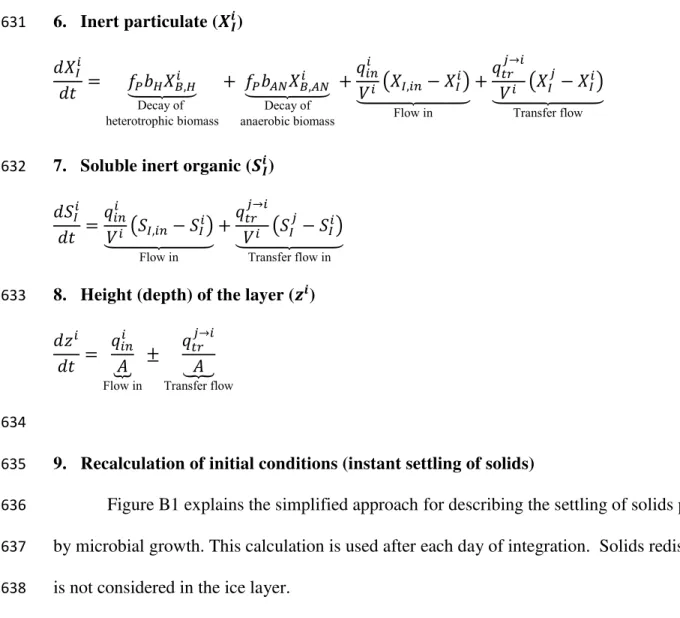
6. Inert particulate (��) 631 ��� � = ⏟ Decay of ��, heterotrophic biomass + ⏟ ����,�� Decay of anaerobic biomass +�⏟ ���� (��,� − ���) Flow in +��� →� �� (�� − ���) ⏟ Transfer flow
7. Soluble inert organic (��) 632 �� � = ��� �� ( �,� − ��) ⏟ Flow in +��� →� �� ( � − ��) ⏟ Transfer flow in
8. Height (depth) of the layer (��) 633 �� � = ��� � ⏟ Flow in ± ��� →� � ⏟ Transfer flow 634
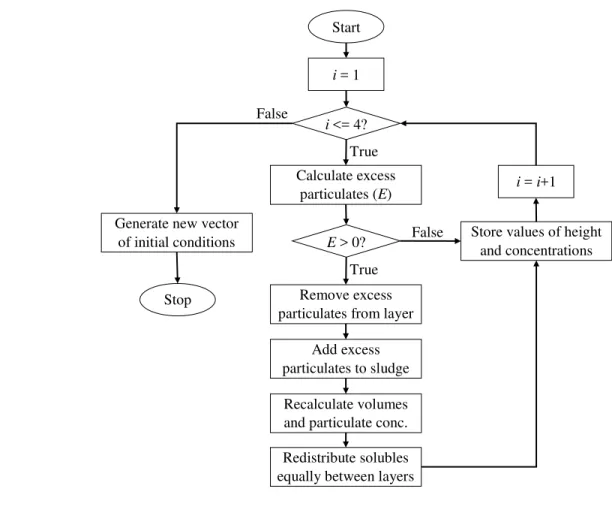
9. Recalculation of initial conditions (instant settling of solids) 635
Figure B1 explains the simplified approach for describing the settling of solids produced
636
by microbial growth. This calculation is used after each day of integration. Solids redistribution
637
is not considered in the ice layer.
639 640 641 642 643 644 645 646 647 648 649 650 651 652 653 654 655 656 657
Figure B1. Flow chart describing the particulates and solubles redistribution between layers for
658
the simulation of instant solids settlement (where � = , , ��). Note: Excess particulates are
659
transferred to the sludge layer without affecting the anaerobic liquid layer.
660 661 i = 1 Start i <= 4? True False Stop Calculate excess particulates (E) E > 0? True i = i+1 False Remove excess particulates from layer
Add excess particulates to sludge Recalculate volumes and particulate conc. Redistribute solubles equally between layers Generate new vector
of initial conditions Store values of height and concentrations
10. Flow rates distribution 662
Input wastewater is distributed between the aerobic, ice, anaerobic, and sludge layers by using
663
the following conditions for selecting the flow rate between layers.
664
Condition Time Layer thickness Input flow Transfer flow
1. No icecap � ∈ [ , �� � ���) or � ∈ ����, ] ��� � > ����∗ = −� �� ����∗= −� �� ���∗= ��� ����� = �����→�� = −����∗ �����←�� = ����∗ 2. Icecap formation � ∈ [�� ���� , �� ����+ Δ�� ����) ��� � > ���� = ���� = ����∗ ��� = ���∗ ����� = ����∗ �����→��� = ����∗− � ������←�� = −����∗+ � 3. Icecap saturation � ∈ [�� ����+ Δ�� ���� , ���� − Δ����) ��� � > ��� ��→��� = � ���∗ ������←�� = −����∗ 4. Icecap melt � ∈ ���� − Δ���� , ����] ��� � > �����←��� = ����∗+ � ������←�� = −����∗ − � 4. Icecap limited � ∈ [�� ����, ����] ��� � = ���� � < � �� ��� ���� = ���� = ��� = ���∗ ����� = ����∗+ ����∗ None where � = � Δ� �· ������ − ����� and � = � Δ� � · ���� ���� − Δ���� − ����� 665 666 667 668 669