Projecting Basin-Scale Distributed Irrigation and Domestic Water Demands and Values: A Generic Method for Large-Scale Modeling

HAL Id: hal-01425103

https://hal-enpc.archives-ouvertes.fr/hal-01425103

HAL is a multi-disciplinary open access archive for the deposit and dissemination of sci-entific research documents, whether they are pub-lished or not. The documents may come from teaching and research institutions in France or abroad, or from public or private research centers.

L’archive ouverte pluridisciplinaire HAL, est destinée au dépôt et à la diffusion de documents scientifiques de niveau recherche, publiés ou non, émanant des établissements d’enseignement et de recherche français ou étrangers, des laboratoires publics ou privés.

Projecting Basin-Scale Distributed Irrigation and

Domestic Water Demands and Values: A Generic

Method for Large-Scale Modeling

Noémie Neverre, Patrice Dumas

To cite this version:

Noémie Neverre, Patrice Dumas. Projecting Basin-Scale Distributed Irrigation and Domestic Water Demands and Values: A Generic Method for Large-Scale Modeling. Water Economics and Policy, 2016, 2 (4), pp.1650023. �10.1142/S2382624X16500235�. �hal-01425103�

Projecting basin-scale distributed irrigation and

domestic water demands and values: a generic

method for large-scale modeling

Noémie Neverre

_{, Patrice Dumas}

a_{Centre International de Recherche sur l’Environnement et le Développement (CIRED), Campus du} Jardin Tropical, 45 bis avenue de la Belle Gabrielle, 94736 Nogent sur Marne, France,


b_{CentreNational de la Recherche Scientifique (CNRS), 3 rue Michel-Ange, 75016 Paris, France} c

École Nationale des Ponts et Chaussées (ENPC), Cité Descartes, 6-8 avenue Blaise Pascal, 77455 Champs-sur-Marne, France

d

Centre de coopération Internationale en Recherche Agronomique pour le Développement (CIRAD), 42 rue Scheffer, 75016 Paris, France


Abstract

This paper presents a methodology to project irrigation and domestic water demands on a regional to global scale, in terms of both quantity and economic value. Projections are distributed at the water basin scale. Irrigation water demand is projected under climate change. It is simply computed as the difference between crop potential evapotranspiration for the different stages of the growing season and available precipitation. Irrigation water economic value is based on a yield comparison approach between rainfed and irrigated crops using average yields. For the domestic sector, we project the combined effects of demographic growth, economic development and water cost evolution on future demands. The method consists in building three-part inverse demand functions in which volume limits of the blocks evolve with the level of GDP per capita. The value of water along the demand curve is determined from price-elasticity, price and demand data from the literature, using the point-expansion method, and from water cost data. This generic methodology can be easily applied to large-scale regions, in particular developing regions where reliable data are scarce. As an illustration, it is applied to Algeria, at the 2050 horizon, for demands associated to reservoirs. Our results show that domestic demand is projected to become a major water consumption sector. The methodology is meant to be integrated into large-scale hydroeconomic models, to determine inter-sectorial and inter-temporal water allocation based on economic valuation.

Keywords: Water demand projection; water value; large-scale modeling; domestic water demand;

irrigation water demand.

1 Introduction

Water resources are already under pressure in some regions of the world, and are facing increasing pressures caused by global socioeconomic and environmental changes. This issue is particularly acute in the Mediterranean, where demographic and economic growth is expected to increase water demands in the coming decades, while climate change is predicted to negatively affect the water supply (Barros et al., 2014). In this context, there is a need for water resources assessments, to anticipate future scarcity issues.

It would be relevant for these assessments to maintain a double focus: a large-scale coverage, and a representation of spatial heterogeneity at the river basin level. Large-scale coverage allows for the representation of interactions between basins with heterogeneous

profiles (water transfers, virtual water trade etc.); it can also address global changes and their impacts on water resources (Alcamo et al., 2003; Haddeland et al., 2011; Hanasaki et al., 2013a, 2013b; Schewe et al., 2014; Strzepek et al., 2013; Wada et al., 2014). In contrast, water resources are managed at the river basin scale, and, depending on the river basin’s characteristics, the local impacts of global changes may be different.

It is also relevant to consider both water quantities and water values. Water management policies are increasingly encouraged to consider water as an economic good (ICWE, 1992). Water basin management requires being able to measure the economic benefits associated with water uses, and the changes in benefits associated with a change in water allocation or availability. Economic valuation can provide valuable information on how to manage the available water as efficiently as possible. Hydroeconomic models address the issues of water allocation between competing uses as well as intertemporal allocation. Water is allocated between its different uses based on the economic benefits they generate, the objective being to maximize the expected aggregated economic value of the water used (Harou et al., 2009).

With this in mind, our objective is to project future water demands and their economic values to 2050, in a framework combining river basin level modeling with an extended geographic coverage. In the present paper we focus on two main sectors of water use: the agricultural sector, and the domestic sector. Irrigation is the major water consumption sector in many regions of the world; in the Mediterranean basin it represents 65% of total water use, and up to 80% in its southern rim (Margat and Treyer, 2004). Since livestock water use is much smaller than irrigation water use (Alcamo et al., 2007; Hanasaki et al., 2013a), in the present paper we consider only irrigation water needs. Domestic demand is the second largest consumption sector of the Mediterranean basin, representing 13% of total water use; moreover, it is critical in terms of needs, and its share in total demand is increasing.

A number of studies have addressed the issue of water demand projection on a large scale: Döll and Siebert (2002); Biemans et al. (2011) for irrigation water, Ward et al. (2010) for municipal and industrial water, Alcamo et al. (2003); Hanasaki et al. (2013a); Strzepek et al. (2013) for both agricultural and non-agricultural sectors. For agricultural water demand, two different approaches coexist: one based on statistical projections of irrigated areas at the country scale (Shen et al., 2008), and another based on the modeling of crops biophysical water needs (Döll and Siebert, 2002; Alcamo et al., 2003, 2007; Strzepek et al., 2013; Hanasaki et al., 2013a). For the domestic sector, existing projections are mainly based on statistical approaches at the country scale, in which demand evolves with GDP per capita as the country develops. Demand can either be directly estimated as a function of population and GDP per capita (Hughes et al., 2010; Ward et al., 2010), or domestic water use intensity per capita is estimated as a function of GDP per capita (Alcamo et al., 2003; Shen et al., 2008) and is then multiplied by the projected population. Other country-dependent variables (e.g. climatic variables) can also be included in the estimations.

However, the issue of water value has yet to be addressed by the large-scale literature. Determining the value of water in its different uses is complex and requires non-market valuation methods, as described by Young (2005). For producers’ uses, such as agricultural demand, where water is an intermediary good, the main valuation method is the residual method. It consists in isolating the marginal contribution of water to the total value of the final good produced: knowing the value of the output, values of all inputs other than water are

subtracted, and what remains is the residual value of water. For consumers’ uses, such as domestic demand, where water is a final good, the most frequently used approach is statistical. It consists in econometrically estimating demand functions, and deriving consumers’ surplus. Such methods are very data intensive. Large-scale data availability is low and implementing methods as precise as what can be done at the water basin scale proves difficult on a large scale. This could be one of the reasons why hydroeconomic models have mostly been developed at sub-national scales (Harou et al., 2009).

To fill this need, this paper presents a methodology designed to project both water demands and values under global changes, and suitable for a large-scale region with heterogeneous data availability such as the Mediterranean. The methodology is thus generic, and easily transposable to other large-scale regions of application. It is meant to be integrated into the ODDYCCEIA1 water-modeling framework (Portoghese et al. (2013), section 9.4), in order to form a generic large-scale hydroeconomic model.

Irrigation water demand is modeled using a biophysical approach, following Döll and Siebert (2002). For irrigation water valuation, we propose a simple method derived from the residual method, using only globally available data. For the domestic sector, we have developed a generic method in which an approach similar to that of WaterGAP (Alcamo et al., 2003, 2007) is incorporated into a simple demand function estimation framework in order to project both demands and values. Demands are located and associated to reservoirs and water basins using the ODDYCCEIA methodology (Portoghese et al., 2013). Therefore, only demands that could be satisfied by large reservoirs are taken into account. As an illustration, the methodology is applied to Algeria, covering fifteen basins, at the 2050 horizon.

2 Methodology

The present paper focuses on the demand side of water resources assessment; the supply side is not considered. Therefore, the methodology described below projects potential demands, not actual withdrawals, and more specifically on-site potential demands. To estimate corresponding potential water withdrawals, potential demands would have to be multiplied by efficiency ratios to account for distribution losses.

Future demands and values are projected at the 2050 horizon; the year 2000 is the year of reference for historical conditions.

1

ODDYCCEIA is the name of the framework. The abbreviation stands for Optimal Dam Dimensioning Yield and Climate Change Economic Impact Assessment. The acronym does not necessarily match the current use of the framework. It was coined for the Nassopoulos et al. (2012) paper, dedicated to cost benefit analysis and robust decision making for dam dimensioning adaptation under uncertain climate change. The

ODDYCCEIA framework was also used to analyze imbalances between water supply and irrigation demand in the Mediterranean basin under climate change (Portoghese et al., 2013).

2.1 Irrigation demand projection

Irrigation demand projection followed the methodology of the ODDYCCEIA model (Portoghese et al., 2013). Historical irrigated areas were determined from globally available data on irrigated areas and crops (Siebert et al., 2005), and crop mixes in the different irrigation perimeters were taken from the Agro-MAPS database (FAO, 2005). Future crop surfaces and types were assumed to be the same as in historical conditions (year 2000): we did not model changes in crop type distribution nor in areas equipped for irrigation.

Irrigation requirements were defined as the deficit between potential crop evapotranspiration and effective precipitation (irrigation to the potential). Effective precipitation was computed following Döll et al. (2003). Crop evapotranspiration was computed for the different stages of the growing season using the method proposed by Allen et al. (1998). The AQUASTAT Programme (2007) was used for crop calendars, and the duration of growth phases was assumed to remain the same in the future. The reference evapotranspiration (ET0) was computed following the Hargreaves method. Crop

evapotranspiration (ETc) was then determined using crop coefficient (Kc) values from Allen et al. (1998): 𝐸𝑇𝑐 = 𝐸𝑇0× 𝐾𝑐.

For each crop c located in perimeter l and for each month m, the monthly irrigation water demand Wc,l,m is:

𝑊_{𝑐,𝑙,𝑚}= [∑(𝑑𝜑,𝑚× 𝐸𝑇0𝑔× 𝐾𝑐𝜑,𝑐)

𝜑

− 𝑃_{𝑒𝑓𝑓𝑔}] × 𝐴𝑐

with dφ,m the number of days of each growth stage φ in month m, ET0 the daily reference

evapotranspiration, Peff the monthly effective precipitation, g the nearest climatology grid

point, Kcφ,c the crop coefficient for phase φ and crop c, and Ac the crop area equipped for

irrigation.

Future irrigation needs are affected by climate change. Climatic data were taken from the Centre National de Recherches Météorologiques (CNRM) climatic model (Dubois et al., 2012), under the A1B IPCC-SRES emission scenario. The CNRM climatic model uses a stretched-grid global climate model zoomed on the Mediterranean, coupled with a high resolution oceanic model of the Mediterranean. This model therefore has a combination of resolution and feedbacks that are lacking in more classical experiments. Runs under Representative Concentration Pathways forcings are not yet available in this setup.

Sixteen types of crops are differentiated in the ODDYCCEIA methodology: cotton, fodder, fruits, maize, oil-seed, oil-tree, potatoes, pulses, rice, rubber, sorghum, sugar beet, sugarcane, tobacco, vegetables and wheat.

2.2 Irrigation water value

2.2.1 Yield comparison approach

We estimated irrigation water value based on a “yield comparison approach” (Turner, 2004), a simple approach derived from the residual method (Young, 2005). Respective costs and benefits of rainfed and irrigated production were compared. For a given crop in a given

costs. The value of water consists in the additional net benefits associated with the use of water.

We computed the value of water for each ODDYCCEIA crop type, in each irrigation perimeter location (i.e. at the 0.5°per 0.5°grid cell scale), as follows:

𝑉 =𝐵𝑖𝑟− 𝐵𝑟𝑓 𝑊

where V is the volumetric value of irrigation water (in USD/m3). Bir is the net benefit

obtained by the irrigated production of a given crop in a given location (in USD/ha), and Brf

is the net benefit that would be obtained if this crop was rainfed. W is the quantity of water used for irrigating the crop in this irrigation perimeter (in m3/ha). V can be negative if the additional profits generated by irrigation do not offset its additional costs. In this case, rainfed production is preferable to irrigated production. We assume that, for a given crop in a given location, production costs (fertilizers, labor etc.) are identical2 for an irrigated or a rainfed crop, and that the only difference in costs between rainfed and irrigated production comes from the cost of irrigation (investment, operation and maintenance costs). This enables us to compute the value of water despite the lack of data on agricultural production costs. It gives a simple expression of the value of water:

𝑉 =(𝑌𝑖𝑟− 𝑌𝑟𝑓) × 𝑃 − 𝐶𝑖𝑟 𝑊

where Yir and Yrf are irrigated and rainfed crop yields (in tons/ha), P is the price of the crop

(in USD/ton), Cir is the cost of irrigation (in USD/ha) and W is the quantity of water used for

irrigation (in m3/ha). The following paragraphs describe how the different terms of this expression were computed.

Irrigation needs (W) are estimated following the methodology described in Section 2.1. In this methodology, irrigated crops are assumed to be irrigated to the potential.

2.2.2 Prices and costs

Crop prices (P) were taken from country scale FAOSTAT data (FAO, 2013), for a representative crop for each ODDYCCEIA crop type. We assume that the price of an irrigated and a rainfed crop is identical. Unfortunately, data are not always available for every year and assumptions may have to be made on a country basis. For the application to Algerian basins, the data used are displayed in Appendix A. For one crop type, sugar beet, the price was not directly available in FAOSTAT data. It had to be reconstructed based on the price of raw sugar from Pink Sheet data (World Bank, 2013). The authors' calculations are described in Appendix B.

2

We assume that both the irrigated and the rainfed crop receive the same quantity of inputs, even if inputs do not have the same efficiency. We also assume that the difference in harvest costs due to the difference in yields is low compared with total cost per

Precise and localized data on irrigation costs (Cir) are not available at the global scale.

Therefore, assumptions had to be made depending on the region of application of the model. For Algeria, we estimated irrigation costs as described in Appendix A.

2.2.3 Yield function

In order to determine irrigated and rainfed yields (Yir and Yrf) under future hydro-climatic

conditions, we modeled yield as a simple function of usable water and ETc.

Figure 1: Modeling crop yield as a function of available water to ETc ratio.

Y

Y

pp the effective precipitation.

The simple piecewise linear yield function (Figure 1) was calibrated for each crop type in each location by means of these two points of reference: the couples (yield of reference, usable water to ETc ratio of reference), for rainfed and irrigated crops. Hence, for each crop type in each irrigation perimeter location, we have to determine i) historical usable water-to-ETc ratios, and ii) historical rainfed and irrigated yields.

For rainfed crops, historical precipitation-to-ETc ratios were computed at the 0.5° per 0.5° spatial resolution. They are based on average precipitation and ETc outputs of the CNRM model (Dubois et al., 2012), calculated over fifty past climatic years. For irrigated crops, by construction usable water-to-ETc ratio is always equal to one (Figure 1).

Lund-Potsdam-Jena managed Land (LPJmL) (Bondeau et al., 2007) provides data on potential and actual yields for rainfed and irrigated crops, at the 0.5° per 0.5° spatial resolution, on a global scale. This data is available only for a certain number of crop types. We therefore used two different methodologies to reconstruct crop yields of reference, depending on crop types.

For ODDYCCEIA crop categories matching LPJmL crop types (Appendix C), we used LPJmL data. Data were first corrected for inconsistencies3. Then, to make sure that the difference in yield between irrigated and rainfed crops was due only to the water used, and not to differences in inputs or soil quality, we did not use actual irrigated yields from LPJmL. Instead, we used potential irrigated yields, corrected by the same actual-to-potential yield gap ratio as the one observed for rainfed yields. Yield gap ratios between potential and actual rainfed yields are very variable between crops and grid cells. In order to reduce possibly unrealistic heterogeneities, we defined both irrigated and rainfed yields of reference as LPJmL potential yields scaled by the average actual-to-potential yield gap ratio. The average yield gap ratio was computed across all rainfed crops at the country scale. Finally, for each crop in each location the yields of reference were calculated as: 𝑌𝑟𝑒𝑓,𝑟𝑓 = 𝑌𝑝𝑜𝑡,𝑟𝑓× 𝑟̅𝑌𝑔𝑎𝑝, and

𝑌_{𝑟𝑒𝑓,𝑖𝑟} = 𝑌_{𝑝𝑜𝑡,𝑖𝑟}× 𝑟̅_{𝑌𝑔𝑎𝑝}, where 𝑟̅_{𝑌𝑔𝑎𝑝} is the average yield gap ratio between potential and actual yields, and Yref and Ypot are yields of reference and potential yields for rainfed (rf) or

irrigated (ir) crops.

For the other crop categories, data on localized yields are not available. We therefore used data on national production and area per crop from FAOSTAT (FAO, 2013), which we aggregated to match our crop categories (Appendix C), under a simple assumption on yield ratios in order to reconstitute irrigated and rainfed yields. We assume that a country’s total agricultural production for a crop type is:

𝑄

= 𝑄

+ 𝑄

= 𝑌̅

× 𝑆

+ ∑ 𝑌

𝑐𝑒𝑙𝑙𝑠

× 𝑆

where Qtot is the total quantity produced (in tons), Qrf,tot and Qir,tot are total rainfed and

irrigated productions (in tons), Srf,tot is the total rainfed area (in ha) and 𝑌̅𝑟𝑓 is the mean rainfed

yield (in tons/ha) in the country. Sir,cell and Yir,cell are the irrigated area and the irrigated yield in

each grid cell of 0.5° per 0.5°. Then, we assume that in every grid cell:

𝑌

= 𝑌̅

×

𝐸𝑇𝑃

𝑝𝑝

where ppcell and ETccell are historical precipitation and ETc in the grid cell considered,

calculated over fifty past climatic years. And:

𝑌̅

=

𝑄

𝑆

+ ∑

𝐸𝑇𝑃

𝑝𝑝

𝑐𝑒𝑙𝑙𝑠

× 𝑆

In this way we can determine an average historical rainfed yield and a localized historical irrigated yield per crop type.

The yield data sources used for each ODDYCCEIA crop category and crop type equivalences are displayed in Appendix A and Appendix C.

3

For a given crop in a given grid cell, if potential yield is inferior to actual yield (for both rainfed and irrigated crops) or if potential irrigated yield is inferior to potential rainfed yield, data were corrected so that both yields were equal to the highest value.

Once the simple yield function has been calibrated with the two reference points, future yields can be easily computed for each crop type in each grid cell, as a function of future hydro-climatic conditions (Figure 1): rainfed yield will be a function of future effective precipitation-to-ETc ratio, whereas irrigated yield will always match the potential irrigated yield since by construction the quantity of water used for irrigation is computed as the deficit between precipitation and ETc. To take into account future yield increases associated to an increased use of other inputs, we added a yield change multiplier. Its value was taken from Alexandratos and Bruinsma (2012), for corresponding crop types in Algeria at the 2050 horizon (Appendix A).

As with the residual method, the methodology results in the estimation of average values. For each crop in each location we obtain a past value of irrigation water based on historical yields and climatic conditions, and a future value of irrigation water based on future climatic conditions and yield change multipliers, computed over fifty climatic years. The method is schematized in Figure 2.

Figure 2: Methodology for projecting irrigation demands and values, for each crop type in

each irrigation perimeter

2.3 Projection and valuation of municipal water demand

2.3.1 Building demand functions

For the domestic sector, the value of water is usually evaluated using econometrically estimated demand functions at the basin scale (Arbués et al., 2003). Given the low data availability when working at a large scale, we developed a framework to build generic demand functions (Neverre and Dumas, 2015). Our approach is to build simple three-part inverse demand functions (Figure 3): the first part consists of basic water requirements for consumption and hygiene, which are very highly valued (e.g. drinking water); the second part consists of additional hygiene and less essential uses, which are less valued than those of the

first part (e.g. regular laundry); finally the third part consists of further indoor uses and outdoor uses which are the least valued (e.g. lawn watering).

Then, we allow for the structure of our demand function to evolve over time, in order to take into account the effect of economic development on demand (Figure 3). As GDP per capita increases, households acquire more water using appliances (e.g. washing machines) and demand more water, until they eventually reach equipment saturation and water demand stabilizes even if income continues to grow. This economic development effect was modeled in the WaterGAP model (Alcamo et al., 2003). We used a similar methodology, but incorporated it into our economic demand function framework: the size of the blocks of the demand function are scaled by economic development. The width of the second and third blocks grows with the level of GDP per capita, as illustrated in Figure 3. This relation between GDP per capita and the width of the blocks was statistically calibrated at the country scale. We assume that basic needs are not affected by this equipment effect, and the width of the first block is assumed fixed and is based on the literature (Howard and Bartram, 2003; Gleick, 1996).

The willingness to pay was estimated for some demand points of reference, based on econometric studies (Nauges and Thomas, 2000; Schleich and Hillenbrand, 2009; Frondel and Messner, 2008) and price data (domestic water prices, bottled water prices), then interpolated linearly to form the slopes of the blocks.

Demand can be projected for a given year t following these steps: first, determine the potential demands of the second and third blocks (Q2 and Q3) depending on the level of GDP

per capita in year t, in order to build the economic demand function for the year t. Second, project the price for year t, and determine the actual level of demand for that level of price, based on the economic demand function (Figure 4). Then the value of water can be computed: it consists of the economic surplus, i.e. the difference between willingness to pay and the actual cost of water (Figure 4).

The domestic demand functions modeled here account for both household uses and commercial and collective uses.

Unlike Alcamo et al. (2003), we did not specifically model technical change. The statistically estimated relation between GDP per capita and demand blocks width accounts for both structural change effects and embedded technological change effects that may have slowed down demand increase as the country developed. As a result, once a country reaches demand saturation there is no further technological change. Demand per capita can however decrease due to price effects. This issue is further discussed in Neverre and Dumas (2015).

Figure 3: Domestic water demand function: economic development effect. Q₁, Q₂ and Q₃ are the volume limits of the three demand parts. The gray arrows represent the effect of economic development, which leads to larger demand by expanding the width of the blocks.

Figure 4: Domestic water demand function: surplus. D is the level of demand corresponding to the level of price. The gray-colored area under the curve represents total economic surplus.

2.3.2 Spatial distribution

The localization and population distribution of current urban areas were taken from the Global Rural-Urban Mapping Project (GRUMP) database (Center for International Earth Science Information Network (CIESIN) et al., 2004). We assume that the localization of future urban areas remains the same as in 2000, and that future population growth is homogeneously distributed among existing locations (i.e., the population ratio of each city over the total population remains unchanged).

2.4 Demand-reservoir-basin association

Agricultural demands and values were computed at a thirty-minute spatial resolution, and then aggregated at the basin scale. Domestic demands and values were computed at national scale, and then distributed at the basin scale. The basin-scale distribution of demands was performed as follows. Q₁ Q₂ Q₃ Willingness to pay (USD/m3₎ Quantity (litre/capita/day) Q₁ Q₂ Q₃ Willingness to pay (USD/m3₎ Quantity (litre/capita/day) Price Cost D

To associate demands with basins, we first associated reservoirs to basins and then demands to reservoirs. Reservoirs were located using the AQUASTAT Programme (2007). Associations of demands to reservoirs are not known at a country or regional level. To reconstruct reservoir-demand links, we used a method based on topological constraints with a penalization of distance covered and altitude difference of ascending moves, along the supply-demand path. Water balance constraints on the network mean annual supply and consumptive demand were also taken into account while minimizing the total cost of associations (Portoghese et al., 2013). Demands associated to a reservoir can potentially be situated in an adjacent basin.

3 Application to Algeria

The methodology projects demands, not withdrawals. In order to convert demands into withdrawals, efficiency ratios from Margat and Treyer (2004) can be used. According to this source, in Algeria the historical demand-to-withdrawal ratio, accounting for distribution losses, is 50% for both irrigation and domestic water. Domestic sector efficiency is about 78.5% and 69% for Moroccan and Tunisian demands in cross-border basins.

3.1 Evaluation in historical conditions

For the domestic sector, an evaluation of the methodology is available in Neverre and Dumas (2015).

For the irrigation sector, we compared the potential demands we modeled for historical conditions to historical data gathered by SIMEDD (Plan Bleu, 2012). In Algeria, historical irrigation withdrawals range from 1.8 to 4 km3/year, for the years 2000 to 2002. Our modeled historical potential demand for Algeria4 is 19 km3/year, which represents a potential withdrawal of 38 km3/year. There are three reasons why potential demand may be much larger than actual irrigation. First, we model irrigation needs required to irrigate to the potential. In fact, crops are not irrigated to the potential because demand is constrained by available water and also because crops can tolerate some level of water constraint. Second, not all areas equipped for irrigation do actually irrigate. Benmouffok (2004) notes that for areas desigated as large irrigation perimeters (“grands périmètres irrigués”) in Algeria, irrigated areas represent only about 25% of areas equipped for irrigation. Third, some irrigation perimeters rely on groundwater, especially Saharan basins where there is pumping of fossil groundwater. The present paper focuses on the demand side and therefore offers a projection of potential demands, both for the municipal and the irrigation sectors. In future developments of the framework, the supply side will be taken into account: potential demands will be compared to available water resources in order to evaluate withdrawals.

Aylward et al. (2010) gathered water value estimations from various studies, in various countries, for the different sectors. The estimations show that on average domestic water uses have higher values than irrigation uses. However, there is a large variability between results obtained in the different studies, which were carried out in different countries and with

4

various methodologies. For the agricultural sector the value of water ranges from 0 to 2 USD/m3.

In Algeria, a large part of our projected irrigation water values falls within that range, with an average value of 0.85 USD/m3, but we also have some irrigation uses with higher values. The maximum value obtained is 60.68 USD/m3, but it is not very representative since only 1.6% of irrigation water demands have a value higher than 10 USD/m3. 15% of irrigation water demands have a value higher than 2 USD/m3, and 5% lower than -0.1 USD/m3. The minimum value is -0.95 USD/m3.

3.2 Projection scenarios

Crops' future water needs, yields and water values were determined for each crop type in each irrigation perimeter, depending on average future climatic conditions from fifty future climatic years of CNRM model (Dubois et al., 2012) outputs, for the A1B IPCC-SRES emission scenario. The irrigation water value was computed under two different scenarios of future crop prices evolution: either crop prices remained equal to present prices, or crop prices increased in the future. The price increase scenario followed Nexus Land Use model (Souty et al., 2012) outputs for a baseline scenario (Brunelle et al., 2015), as described in Appendix D.

A domestic water demand projection was performed using the SSP2 Shared Socioeconomic Pathways (Rozenberg et al., 2014) for GDP evolution, combined with the medium population projection scenario from the UN (UN, 2009). Water cost and water price were assumed to increase over time along with the following scenario (Neverre and Dumas, 2015): the cost of water increases with GDP per capita, towards the cost of a mature water distribution and sewerage service (the current cost level in France was chosen as a representative target cost of reference); the cost-recovery ratio converges towards one as GDP per capita grows. Water cost reaches the target cost level and the cost-recovery ratio reaches one when GDP per capita reaches the reference level of GDP per capita in France. A sensitivity analysis was also performed for domestic water demand, by selecting two other Shared Socioeconomic Pathways and two other population projection scenarios from the UN, low and high variants.

3.3 Projection results

The area of application covers fifteen basins (Figure 5). Among these, one is an “internal drainage” basin (basin 1), which does not outflow to the sea and corresponds mostly to desert; the remainder are coastal basins (basins 2 to 15). Results of projected demands and values are presented in Table 1 for an overview of all fifteen basins, and in Figure 6 and Figure 7 for a closer look at the respective values of domestic and irrigation water in two representative basins.

Figure 5: Map of Algerian basins, labeled 1 to 15. Basin borders are in black, and Algerian borders in white. The Mediterranean Sea is the white area. White dots represent cities of more

than 100,000 inhabitants. Basin 2 is a basin located in western Algeria, that flows mostly through Morocco to the Atlantic Ocean and is outside the scope of this map.

Looking at the region as a whole, results show that both domestic demand and irrigation demand will increase in the future. Domestic demand becomes a major consumption sector at the 2050 horizon. Its share in total demand (domestic demand plus potential irrigation demand) increases from 16% under historical conditions to 35-45% in 2050, depending on socioeconomic scenarios (Table 1). Indeed, the domestic demand increase could range from +200% to +358% by 2050, while irrigation demand is modeled to increase by 8% under future climatic conditions (A1B SRES scenario) with constant irrigated areas.

Results differ significantly between the two different types of basins. This contrast is illustrated with projection results for basins 1 and 4 (Figure 6 and Figure 7). Basin 1 is a very large basin, located in the arid part of Algeria. Runoff is infiltrated and evaporated, and the basin does not outflow to the sea. Basin 4 is one of the smaller basins located in the coastal part of Algeria. They are both cross-border basins (Figure 5).

Figure 6 and Figure 7 show annual sectorial water demands at the basin scale, ordered by decreasing value. The three-part structure of our domestic demand-function modeling framework is identifiable, with high valued basic uses, followed by less valued intermediate uses, and finally least-valued supplementary uses.

In basin 4 (Figure 6), total domestic demand (coming from both Algerian and Moroccan cities) outweighs irrigation demand in 2050. The value of irrigation water is very low compared with the value of domestic water. For Algerian demand, the domestic water value is always higher than the irrigation water value; for Moroccan demand, only some least-valued domestic uses have a value comparable to the irrigation water value.

Figure 6: Projected domestic and irrigation demands in Basin 4, for year 2050, under the following scenarios: F-med (i.e. medium population variant and SSP2) for domestic demand,

and F-0 (i.e. no price increase) for agricultural demand. In order to facilitate reading the figure and comparing values, the maximum value reached by irrigation water uses is

highlighted.

In basin 1 (Figure 7), future irrigation water needs remain much higher than total domestic demand. Irrigation water can have a very high value for some crops, comparable to the values of second-block domestic demands (or even first-block domestic demands, in some exceptional cases). One reason may be that in this arid zone crop production is null without irrigation, while with irrigation there is no limitation by radiation. In this basin, water allocation based on economic criteria could favor some irrigation demands over non-essential domestic demands.

Population is predominantly distributed in the coastal water basins, where irrigation demand is lower than domestic demand (e.g. basin 4, where Oran, the second largest city of Algeria, is located). Irrigation demands are larger in less-populated areas (e.g. basin 1). The priority given to domestic needs over agriculture can impact the quantity of water allocated to irrigation within a basin, but it can also impact longer-term investment decisions, such as which areas to equip for irrigation, in which basins.

Figure 7: Projected domestic and irrigation demands in Basin 1, for year 2050, under the following scenarios: F-med (i.e. medium population variant and SSP2) for domestic demand,

and F-0 (i.e. no price increase) for agricultural demand. In order to facilitate reading the figure and comparing values, the maximum value reached by irrigation water uses is

highlighted.

The impacts of different socioeconomic scenarios on future domestic demand are illustrated in Figure 8, compared with modeled historical domestic demand. In historical conditions, the third block of domestic demand is small (Morocco) or even non-existent (Algeria). As countries develop and equipment grows, this third-block demand increases. Our results for future projections show that the total quantity demanded is more sensitive to socioeconomic scenarios than is the value of water.

Figure 8: Projected domestic demand in basin 4, under historical conditions for year 2000,

and under three socioeconomic scenarios for year 2050. Scenarios: F-med (i.e. medium population variant and SSP2), F-low (i.e. low population variant and SSP4) and F-high (i.e.

Table 1: Domestic and agricultural demands and values in Algerian basins. Comparison between modeled historical values and projections at the 2050 horizon under various scenarios. Scenarios for the future are, for the domestic sector: “F-med” = Medium population variant & SSP2; “F-high”= High

population variant & SSP5; “F-low” = Low population variant & SSP4. For agriculture: “F-0” = no crop prices increase; “F-1” = baseline crop prices increase scenario.

Basin

Domestic sector Irrigation sector

Total demand (Million m3_/year)

Total value of water (Million USD2005/year)

Total demand (Million m3_/year)

Total value of water (Million USD2005/year)

Historical F-med F-low F-high Historical F-med F-low F-high Historical F-0 and F-1 Historical F-0 F-1

1 85.1 283.8 255.9 390.0 12,355.8 21,005.4 18,276.6 24,792.7 1,177.2 1,218.3 2,026.5 3,115.7 11,915.2 2 10.4 43.3 36.6 49.7 1,206.2 1,866.3 1,602.7 2,141.2 170.1 180.6 5.4 13.9 89.6 3 11.7 48.8 41.3 56.1 1,360.6 2,105.3 1,807.9 2,415.4 87.7 97.7 2.1 9.8 69.0 4 90.3 316.9 279.8 414.8 12,330.7 20,555.2 17,826.3 24,137.8 173.5 197.6 18.4 42.6 227.1 5 57.4 175.5 161.0 255.7 8,620.2 14,910.6 12,990.6 17,698.2 202.6 239.8 16.0 44.9 258.7 6 112.0 342.5 314.2 498.9 16,821.9 29,097.1 25,350.4 34,537.0 117.1 130.1 13.9 31.4 161.5 7 12.9 39.6 36.3 57.7 1,944.8 3,364.0 2,930.8 3,992.9 18.7 20.2 3.1 6.0 26.8 8 15.5 47.3 43.4 68.9 2,323.3 4,018.7 3,501.2 4,770.0 32.5 35.7 1.7 6.2 33.1 9 7.3 22.4 20.6 32.7 1,102.1 1,906.4 1,660.9 2,262.8 2.1 2.2 0.1 0.3 1.6 10 21.8 66.6 61.1 97.0 3,271.1 5,658.0 4,929.4 6,715.8 10.2 12.2 0.5 2.4 14.5 11 9.2 28.2 25.9 41.1 1,384.7 2,395.2 2,086.8 2,843.0 2.3 2.6 0.5 0.9 4.3 12 29.2 89.3 81.9 130.1 4,385.6 7,585.9 6,609.1 9,004.1 39.5 45.3 9.7 18.2 81.7 13 13.2 60.1 52.4 69.8 1,769.9 2,795.5 2,427.9 3,205.9 29.4 33.8 9.0 17.2 76.7 14 17.9 77.2 67.7 92.5 2,458.1 3,951.5 3,434.0 4,563.3 259.8 298.5 54.0 103.5 459.2 15 5.5 26.1 22.7 29.8 733.2 1,144.9 993.9 1,306.8 285.6 306.6 44.7 81.4 348.6 All 499.4 1,667.6 1,500.8 2,284.8 72068.3 122,359.9 106,428.5 144,386.9 2,608.2 2,821.4 2,205.5 3,494.5 13,767.6

4 Discussion and conclusions

The methodology developed here makes it possible to project the combined impacts of population growth, economic development and water costs on future domestic water demands, and the impact of climate change on future irrigation water demands, in terms of both quantity and economic benefits.

Our results show that the domestic sector will become a major sector of water consumption in 2050, catching up with the irrigation sector. This trend is similar to the results of Alcamo et al. (2007), which is not surprising since we rely on similar assumptions (e.g. we do not model increases in irrigated areas).

With our methodology, irrigation needs increase by 8% under climate change (A1B scenario) in Algeria. The assumption of constant irrigated area could prove to be wrong in 2050. However, at the present time many areas equipped for irrigation are not actually irrigated, and the increase in irrigated areas is constrained by water availability. Increasing irrigation areas would require infrastructure investments, which could be possible in Algeria although the country is already well covered by reservoirs. In our methodology, data on crop mixes are currently taken from Agro-MAPS (FAO, 2005), which leads to an overestimation of areas of irrigated wheat as we do not select crops that are most likely to be irrigated. In our basins of application, there should be more irrigated vegetables and fruits, and less irrigated wheat. The consequence of this discrepancy could be an underestimation of the total value of irrigation water, since vegetable and fruits tend to be more water limited and high value-added crops. In future work, we could use crop mix data from MIRCA2000 (Portmann et al., 2010).

In general, water values are very different between uses, the highest being domestic water values. With our results for Algeria, value estimations come close to simple ranking rules between uses, such as what is implemented by Strzepek et al. (2013). If total demand cannot be met, they allocate water between the different uses based on absolute priorities: the domestic and industrial sectors are the first to be satisfied, then come irrigation and livestock uses. For Tunisia and Morocco, the projected increase in GDP per capita leads to a demand for domestic water extending to low-value uses (Figure 6 and Figure 7). For such uses, trade-offs with irrigation uses are possible. It must also be noted that a correct valuation of water is important for intertemporal prudential allocation rules, to measure correctly the expected water value.

The methodology developed requires calibration. If the necessary data are not available, assumptions will be needed. These assumptions will be made depending on the available data for the location of application considered. In order to project domestic demands and values in a region other than the Mediterranean, other econometric estimations of demand sensitivity to price would be needed and the countries used as a reference in the absence of data would be different (Neverre and Dumas, 2015). In order to determine irrigation costs, Inocencio et al. (2007) could provide information about investment costs in many developing countries. For irrigation perimeter operating costs, there is no large-coverage data source, therefore specific assumptions and data would be needed.

In light of the global coverage, but also lack of precision at the local level, our methodology is meant to represent local impacts of global changes, by bringing together

global and local approaches from the literature. It is however not suitable to build a detailed representation for operational purposes. In the next step, this demand modeling methodology will be integrated into the ODDYCCEIA water model framework (Portoghese et al., 2013), in order to build a generic hydroeconomic model bringing together demand and supply sides. The modular and generic nature of the framework, which only requires globally available data, makes it suitable to apply to diverse regions, in particular to developing regions with low data-availability. This model could be applied to the study of any issue requiring a wide area, such as virtual water trade, evolution of the energy sector water use, or activities and population relocalizations due to water supply reduction or water demand value changes.

Acknowledgements

The authors would like to thank the Direction Générale de l’Armement (DGA) for its financial support through a PhD grant.

Appendix

A Data sources for the application to Algeria

Crop yields and crop prices data sources are displayed in Table 2. For crop prices, data are not always available for every year. Year 2000 is the year of reference for the historical period. If no data are available for year 2000, we select a representative year among those for which data are available: we select a year close to year 2000, avoiding years with extreme values.

We estimate irrigation costs in Algeria as follows. Irrigation costs consist of investment costs plus operation and maintenance costs. We assume that investment costs represent 150 USD/ha/year, which is the average cost for irrigation projects in Algeria, calculated based on Inocencio et al. (2007) with a 5% interest rate and a thirty-year lifetime of the equipment. Data on operation and maintenance costs are very heterogeneous. Based on reports and working papers on irrigation costs in African countries (Perry, 1996; SNC-Lavalin International Inc., 2010; Takeshima et al., 2013), operation and maintenance costs are assumed to represent 150 USD/ha/year on average.

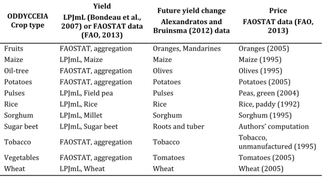
Table 2: Data sources for Algerian crop types

ODDYCCEIA Crop type Yield LPJmL (Bondeau et al., 2007) or FAOSTAT data (FAO, 2013)

Future yield change Alexandratos and Bruinsma (2012) data

Price

FAOSTAT data (FAO, 2013)

Fruits FAOSTAT, aggregation Oranges, Mandarines Oranges (2005)

Maize LPJmL, Maize Maize Maize (1995)

Oil-tree FAOSTAT, aggregation Olives Olives (1995) Potatoes FAOSTAT, aggregation Potatoes Potatoes (2005)

Pulses LPJmL, Field pea Pulses Peas, green (2004)

Rice LPJmL, Rice Rice Rice, paddy (1992)

Sorghum LPJmL, Millet Sorghum Sorghum (1995)

Sugar beet LPJmL, Sugar beet Roots and tuber Authors’ computation Tobacco FAOSTAT, aggregation Tobacco Tobacco, _{unmanufactured (1995)} Vegetables FAOSTAT, aggregation Tomatoes Tomatoes (2005)

Wheat LPJmL, Wheat Wheat Wheat (2005)

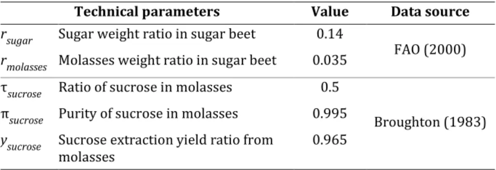
B Computation of the price of sugar beet

Sugar is extracted from sugar beet. In the process, sugar can be obtained directly from the refining of the beet, and then some additional sugar can be obtained from further processing the molasses (refining byproducts). Therefore, we compute the price of sugar beet as follows:

where 𝑃_{𝑅𝑎𝑤𝑆𝑢𝑔𝑎𝑟} is the price of raw sugar (in USD/ton), 𝑟_{𝑠𝑢𝑔𝑎𝑟} and 𝑟_{𝑚𝑜𝑙𝑎𝑠𝑠𝑒𝑠} are the weight ratios of sugar and molasses available in sugar beet, 𝜏𝑠𝑢𝑐𝑟𝑜𝑠𝑒 is the ratio of sucrose in

molasses, 𝜋_{𝑠𝑢𝑐𝑟𝑜𝑠𝑒} is the purity of sucrose in molasses, and 𝑦_{𝑠𝑢𝑐𝑟𝑜𝑠𝑒} is the sucrose yield ratio attainable from molasses. Data sources and values are shown in Table 3.

This price does not take into account transformation costs, nor sugar beet pulp coproduct. Overall, it is probably an overestimation of the sugar beet price.

Table 3: Data used for the computation of sugar beet price

Technical parameters Value Data source

r_sugar Sugar weight ratio in sugar beet 0.14

FAO (2000)

r_molasses Molasses weight ratio in sugar beet 0.035

τ_sucrose Ratio of sucrose in molasses 0.5

Broughton (1983)

π_sucrose Purity of sucrose in molasses 0.995

y_sucrose Sucrose extraction yield ratio from

molasses 0.965

C ODDYCCEIA crop categories: LPJmL crop types

equivalents, and aggregation of FAO crop types

Table 4: LPJmL and FAO crop types and ODDYCCEIA crop categories (nes: not elsewhere specified)

ODDYCCEIA

crop categories LPJmL crops

Maize Maize

Pulses Field pea

Rice Rice

Sorghum Millet Sugar beet Sugar beet

Wheat Wheat

ODDYCCEIA

crop categories FAO crops

Fruits Fruits, fresh nes; Apples; Apricots; Cherries; Figs; Grapes; Oranges; Peaches and nectarines; Pears; Plums and sloes; Quinces; Cherries, sour; Tangerines, mandarins, clementines, satsumas; Dates; Grapefruit (inc. pomelos); Fruit, stone nes; Lemons and limes; Bananas; Plantains; Fruit, citrus nes; Kiwi fruit; Avocados; Persimmons; Mangoes, mangosteens, guavas; Papayas; Pineapples; Tea; Berries nes; Fruit, tropical fresh nes; Cloves; Gooseberries; Raspberries; Blueberries; Cranberries; Coffee, green; Cocoa beans; Coconuts; Kola nuts; Maté; Areca nuts; Vanilla; Fruit, pome nes

Oil-tree Almonds, with shell; Carobs; Hazelnuts, with shell; Olives; Walnuts, with shell; Pistachios; Chestnut; Nuts, nes; Oil, palm fruit; Karite nuts (sheanuts); Cashew nuts, with shell; Cashew apple; Brazil nuts, with shell

Potatoes Potatoes; Sweet potatoes; Roots and tubers, nes; Yams; Cassava Tobacco Tobacco, unmanufactured

Vegetables Cabbages and other brassicas; Carrots and turnips; Cauliflowers and broccoli; Chicory roots; Chillies and peppers, green; Chillies and peppers, dry; Cucumbers and gherkins; Garlic; Lettuce and chicory; Onions, dry; Onions (inc. shallots), green; Pepper (piper spp.); Pumpkins, squash and gourds; Eggplants (aubergines); Strawberries; Tomatoes; Vegetables, fresh nes; Watermelons; Melons, other (inc. cantaloupes); Artichokes; Asparagus; Spinach; Anise, badian, fennel, corian.; Okra; Melonseed; Spices, nes; Currants; Peppermint; Ginger; Mushrooms and truffles; Nutmeg, mace and cardamoms; Cinnamon (canella)

D Scenario of future crop prices increase

Increased crop prices for the year 2050 are taken from Nexus Land Use (NLU) model (Souty et al., 2012) outputs, following the scenario described below (Brunelle et al., 2015). The main scenario variables are the following: food and biofuel consumption, evolution of forest areas, prices of other agricultural inputs. When possible, they are set to reproduce as closely as possible the values provided by Alexandratos and Bruinsma (2012).

Food availability given by the FAO is corrected to include animal fat and exclude fishery products. In 2050, the NLU average food availability amounts to 3727 kcal/capita/day in the OECD countries and the CIS and to 3092 kcal/capita/day in the other countries. With a population growing according to the median scenario projected by the United Nations (UN, 2009), this leads to a global increase in food consumption by 57% over the 2005-2050 period (+1.0% per year).

The biofuel scenario is deduced from the world use of crops for biofuels provided by Alexandratos and Bruinsma (2012). The biofuel production grows from 4 million-tons equivalent of petroleum (Mtep) in 2005 to around 64 Mtep in 2020, and remains constant thereafter. Only first generation biofuels are considered.

In these simulations, the demand for calories is assumed to be inelastic to prices. From this point of view, the results used here can be considered as an upper bound since the possible reduction in food or biofuel demand, due to higher food prices may indeed mitigate the impact on land-use of higher fertilizer price. However, given the weak elasticity of food demand to price5, this effect is thought to be small.

The deforestation rate is exogenously set according to the observed trends over the period 2001-2010 (FAO, 2010), assuming that reforestation that occurs in some regions (such as in the US or China) ceases after 2020. The evolution of total agricultural areas (pasture and cropland area) is directly deduced from reforestation/deforestation rates.

The evolution of fertilizer price is econometrically related with the evolution of oil and gas prices. This equation is estimated over the 1971-2011 period based on World Bank data

5

Biofuel demand is also considered to be weakly price elastic as it is largely driven by national mandates.

(World Bank, 2013). For future projections, oil and gas prices from the Imaclim-R model (Bibas and Méjean, 2014) are used, assuming no climate policy.

Results are available for twelve geographical regions: USA, Canada, Europe, OECD Pacific, Former Soviet Union, China, India, Brazil, Middle-East, Africa, rest of Asia, rest of Latin America. The scenario described above leads to a +3.20% average annual crop price increase rate worldwide, and +2.75% in Africa.

References

Alcamo, J, P Döll, T Henrichs, F Kaspar, B Lehner, T Rösch, and S Siebert (2003). Development and testing of the WaterGAP 2 global model of water use and availability. Hydrological Sciences Journal, 48(3), 317–337.

Alcamo, J, M Flörke, and M Märker (2007). Future long-term changes in global water resources driven by socio-economic and climatic changes. Hydrological Sciences, 52(2), 247– 275.

Alexandratos and J Bruinsma (2012). World agriculture towards 2030/2050. The 2012 revision. Technical report, FAO. ESA Working paper No. 12-03.

Allen, RG, LS Pereira, D Raes and M Smith (1998). Crop evapotranspiration – Guidelines for computing crop water requirements. Technical Report 56, FAO.

AQUASTAT Programme (2007). Dams and agriculture in Africa. Available at: ftp://ftp.fao.org/agl/aglw/docs/Aquastat_Dams_Africa_070524.pdf

Arbués, F, MA García-Valiñas and R Martínez-Espiñeira (2003). Estimation of residential water demand: A state-of-the-art review. The Journal of Socio-Economics, 32(1), 81–102. Aylward, B, H Seely, R Hartwell and J Dengel (2010). The Economic Value of Water for Agricultural, Domestic and Industrial Uses: A Global Compilation of Economic Studies and Market Prices. Technical report, Ecosystem Economics for UN FAO.

Barros, V, C Field, D Dokken, M Mastrandrea, K Mach, T Bilir, M Chaterjee, K Ebi, Y Estrada, R Genova, B Girma, E Kissel, A Levy, S MacCracken, P Mastrandrea and L White (2014). Climate Change 2014: Impacts, Adaptation, and Vulnerability. Part B: Regional Aspects. Contribution of Working Group II to the Fifth Assessment Report of the Intergovernmental Panel on Climate Change. IPCC, Cambridge, United Kingdom and New York, USA, Cambridge university press edition.

Benmouffok, B (2004). Efforts de l’Algérie en matière d’économie de l’eau et de modernisation de l’irrigation. HTE, (130). Communication à l’occasion de la journée mondiale de l’alimentation.

Bibas, R and A Méjean (2014). Potential and limitations of bioenergy for low carbon transitions. Climatic Change, 123(3-4), 731–761.

Biemans, H, I Haddeland, P Kabat, F Ludwig, RWA Hutjes, J Heinke, W von Bloh and D Gerten (2011). Impact of reservoirs on river discharge and irrigation water supply during the 20th century. Water Resources Research, 47. W03509.

Bondeau, A, PC Smith, S Zaehle, S Schaphoff, W Lucht, W Cramer, D Gerten, H Lotze-Campen, C Müller, M Reichstein and B Smith (2007). Modelling the role of agriculture for the 20th century global terrestrial carbon balance. Global Change Biology, 13(3), 679–706. Broughton, D.B. (1983) Sucrose extraction from aqueous solutions featuring simulated moving bed. US Patent 4.404.037.

Brunelle, T, P Dumas, F Souty, B Dorin and F Nadaud (2015). Evaluating the impact of rising fertilizer prices on crop yields. Agricultural Economics, 46(5), 653-666.

Center for International Earth Science Information Network (CIESIN), International Food Policy Research Institute (IFPRI), the World Bank, and Centro Internacional de Agricultura Tropical (CIAT) (2004). Global Rural-Urban Mapping Project (GRUMP): Settlement Points. Palisades, NY: CIESIN, Columbia University.

Döll, P, F Kaspar and B Lehner (2003). A global hydrological model for deriving water availability indicators: model tuning and validation. Journal of Hydrology, 270, 105–134. Döll, P and S Siebert (2002). Global modeling of irrigation water requirements. Water Resources Research, 38(4), 8-1–8-10.

Dubois, C, S Somot, S Calmanti, A Carillo, M Déqué, A Elizalde, S Gualdi, D Jacob, B L’Heveder, L Li, P Oddo, G Sannino, E Scoccimarro and F Sevault (2012). Future projections of the surface heat and water budgets of the Mediterranean Sea in an ensemble of coupled atmosphere-ocean regional climate models. Climate Dynamics, 39(7), 1859–1884.

FAO (2000) Technical conversion factors for agricultural commodities, FAO. Available at: http://www.fao.org/fileadmin/templates/ess/documents/methodology/tcf.pdf

FAO (2005). Agro-MAPS: A global spatial database of agricultural land-use statistics aggregated by sub-national administrative districts. Version 2.5. Available at: http://kids.fao.org/agromaps/

FAO (2010). Global forest resources assessment 2010. Working Papers FAO Forestry paper 163, FAO.

FAO (2013). Food and Agriculture Organisation of the United Nations Statistical database (FAOSTAT). Available at: http://faostat.fao.org/site/339/default.aspx

Frondel, M and F Messner (2008). Price perception and residential water demand: Evidence from a German household panel. In 16th Annual Conference of the European Association of Environmental and Resource Economists, Gothenburg, Sweden.

Gleick, PH (1996). Basic water requirements for human activities: Meeting basic needs. Water international, 21(2), 83–92.

Haddeland, I, DB Clark, W Franssen, F Ludwig, F Voß, NW Arnell, N Bertrand, M Best, S Folwell, D Gerten, S Gomes, SN Gosling, S Hagemann, N Hanasaki, R Harding, J Heinke, P Kabat, S Koirala, T Oki, J Polcher, T Stacke, P Viterbo, GP Weedon and P Yeh (2011). Multimodel estimate of the global terrestrial water balance: Setup and first results. Journal of Hydrometeorology, 12(5), 869–884.

Hanasaki, N, S Fujimori, T Yamamoto, S Yoshikawa, Y Masaki, Y Hijioka, M Kainuma, Y Kanamori, T Masui, K Takahashi S and Kanae (2013a). A global water scarcity assessment under Shared Socio-economic Pathways; Part 1: Water use. Hydrology and Earth System Sciences, 17(7), 2375–2391.

Hanasaki, N, S Fujimori, T Yamamoto, S Yoshikawa, Y Masaki, Y Hijioka, M Kainuma, Y Kanamori, T Masui, K Takahashi S and Kanae (2013b). A global water scarcity assessment under Shared Socio-economic Pathways; Part 2: Water availability and scarcity. Hydrology and Earth System Sciences, 17(7), 2393–2413.

Harou, JJ, M Pulido-Velazquez, DE Rosenberg, J Medellín-Azuara, JR Lund and RE Howitt (2009). Hydroeconomic models: Concepts, design, applications, and future prospects. Journal of Hydrology, 375(3-4), 627–643.

Howard, G and J Bartram (2003). Domestic water quantity, service level, and health. World Health Organization, Geneva, Switzerland.

Hughes, G, P Chinowsky and K Strzepek (2010). The costs of adaptation to climate change for water infrastructure in OECD countries. Utilities Policy, 18, 142–153.

ICWE (1992). Dublin Statement on Water and Sustainable Development. Dublin, Ireland. Inocencio, A, M Kikuchi, M Tonosaki, A Maruyama, D Merrey, H Sally and I Jong (2007). Costs and Performance of Irrigation Projects: A Comparison of Sub-Saharan Africa and Other Developing Regions. Research Report 109, International Water Management Institute.

Margat, J and S Treyer (2004). L’eau des Méditerranéens: Situation et perspectives. Technical Report 158, UNEP-MAP (Mediterranean Action Plan).

Nassopoulos, H, P Dumas and S Hallegatte (2012). Adaptation to an uncertain climate change: Cost benefit analysis and robust decision making for dam dimensioning. Climatic Change, 114(3–4), 497–508.

Nauges, C and A Thomas (2000). Privately operated water utilities, municipal price negotiation, and estimation of residential water demand: The case of France. Land Economics, 76(1), 68–85.

Neverre, N and P Dumas (2015). Projecting and valuing domestic water use at regional scale: A generic method applied to the Mediterranean at the 2060 horizon. Water Resources and Economics, 11, 33-46.

Perry, C J (1996). Alternative approaches to cost sharing for water service to agriculture in Egypt. Technical report, International Irrigation Management Institute, Colombo, Sri Lanka. Plan Bleu (2012). Mediterranean Information System on Environment and Development (SIMEDD). Available at: http://planbleu.org/en/ressources-donnees/simedd.

Portmann, FT, S Siebert and P Döll (2010). MIRCA2000—Global monthly irrigated and rainfed crop areas around the year 2000: A new high-resolution data set for agricultural and hydrological modeling. Global Biogeochemical Cycles, 24(GB1011).

Portoghese, I, E Bruno, P Dumas, N Guyennon, S Hallegatte, J-C Hourcade, H Nassopoulos, G Pisacane, M Struglia and M Vurro (2013). Impacts of climate change on freshwater bodies: quantitative aspects. In Regional Assessment of Climate Change in the Mediterranean: Volume 1: Air, Sea and Precipitation and Water, volume 50 of Advances in Global Change Research, pp. 241–306. A Navarra and L Tubiana, Dordrecht, Springer science and business media edition.

Rozenberg, J, C Guivarch, R Lempert and S Hallegatte (2014). Building SSPs for climate policy analysis: A scenario elicitation methodology to map the space of possible future challenges to mitigation and adaptation. Climatic Change, 122(3), 509–522.

Schewe, J, J Heinke, D Gerten, I Haddeland, NW Arnell, DB Clark, R Dankers, S Eisner, BM Fekete, FJC González, SN Gosling, H Kim, X Liu, Y Masaki, FT Portmann, Y Satoh, T

Stacke, Q Tang, Y Wada, D Wisser, T Albrecht, K Frieler, F Piontek, L Warszawski and P Kabat (2014). Multimodel assessment of water scarcity under climate change. PNAS, 111(9), 3245–3250.

Schleich, J and T Hillenbrand (2009). Determinants of residential water demand in Germany. Ecological Economics, 68(6), 1756–1769.

Shen, Y, T Oki, N Utsumi, S Kanae and N Hanasaki (2008). Projection of future world water resources under SRES scenarios: water withdrawal / Projection des ressources en eau mondiales futures selon les scénarios du RSSE: prélèvement d’eau. Hydrological sciences journal, 53(1), 11–33.

Siebert, S, P Döll, J Hoogeveen, J-M Faures, K Frenken and S Feick (2005). Development and validation of the global map of irrigation areas. Hydrology and Earth System Sciences, 9, 535-547.

SNC-Lavalin International Inc. (2010). Lot 3. O&M system for Kpong irrigation project. Technical report.

Souty, F, T Brunelle, P Dumas, B Dorin, P Ciais, R Crassous, C Müller and A Bondeau (2012). The Nexus Land-Use model version 1.0, an approach articulating biophysical potentials and economic dynamics to model competition for land-use. Geoscientific Model Development, 5(5), 1297–1322.

Strzepek, K, A Schlosser, A Gueneau, X Gao, E Blanc, C Fant, B Rasheed and HD Jacoby (2013). Modeling water resource systems within the framework of the MIT integrated global system model: IGSM-WRS. Journal of Advances in Modeling Earth Systems, 5(3), 638–653. Takeshima, H, K Jimah, S Kolavalli, X Diao and RL Funk (2013). Dynamics of Transformation. Insights from an Exploratory Review of Rice Farming in the Kpong Irrigation Project. IFPRI Discussion Paper 01272, IFPRI, Development Strategy and Governance Division.

Turner, RK (2004). Economic valuation of water resources in agriculture: from the sectoral to a functional perspective of natural resource management. Technical report, Food & Agriculture Org.

UN (2009). World Population Prospects: The 2008 Revision. Working Paper No. ESA/P/WP.210, United Nations, Department of Economic and Social Affairs, Population Division.

Wada, Y, T Gleeson and L Esnault (2014). Wedge approach to water stress. Nature Geoscience, 7(9), 615–617.

Ward, P, K Strzepek, W Pauw, L Brander, G Hughes and J Aerts (2010). Partial costs of global climate change adaptation for the supply of raw industrial and municipal water: a methodology and application. Environmental Research Letters, 5(044011).

World Bank (2013). Commodity Price Data (a.k.a. Pink Sheet) 1960-2013. Available at: http://databank.worldbank.org/data/databases/commodity-price-data.

Young, RA (2005). Determining the economic value of water: concepts and methods. Resources for the Future, Washington, DC, USA.