Analysis and visualization of temporal variations in video

Analysis and Visualization of Temporal Variations in Video

Michael Rubinstein

Submitted to the Department of Electrical Engineering and Computer Science in partial fulfillment of the requirements for the degree of

Doctor of Philosophy in

MASSACHUSETTS INSTIfJTE

Electrical Engineering and Computer Science OF TECHNOLOGY

at the Massachusetts Institute of Technology

APR 10 2014

LIBRARIES

All Rights Reserved.

Author:

Department of Electrical Eng soing and Computer Science November 27, 2013

Certified by: _V

Professor William T. Freeman Thesis Supervisor

Accepted by:

Pr~fessrL 2 ie A. Kolodziejski, Chairmain, Department Committee on Graduate Theses

3

To my parents

Analysis and Visualization of Temporal Variations in Video

by

Michael Rubinstein

Submitted to the Department of Electrical Engineering and Computer Science on November 27, 2013 in Partial Fulfillment of the Requirements for the Degree

of Doctor of Philosophy in Electrical Engineering and Computer Science

Abstract

Our world is constantly changing, and it is important for us to understand how our envi-ronment changes and evolves over time. A common method for capturing and communicating such changes is imagery - whether captured by consumer cameras, microscopes or satellites, images and videos provide an invaluable source of information about the time-varying nature of our world. Due to the great progress in digital photography, such images and videos are now widespread and easy to capture, yet computational models and tools for understanding and analyzing time-varying processes and trends in visual data are scarce and undeveloped.

In this dissertation, we propose new computational techniques to efficiently represent, an-alyze and visualize both short-term and long-term temporal variation in videos and image se-quences. Small-amplitude changes that are difficult or impossible to see with the naked eye, such as variation in human skin color due to blood circulation and small mechanical move-ments, can be extracted for further analysis, or exaggerated to become visible to an observer. Our techniques can also attenuate motions and changes to remove variation that distracts from the main temporal events of interest.

The main contribution of this thesis is in advancing our knowledge on how to process spatiotemporal imagery and extract information that may not be immediately seen, so as to better understand our dynamic world through images and videos.

Thesis Supervisor: William T. Freeman

6

Thesis Committee: Professor Fr6do Durand, Dr. Ce Liu (Microsoft Research), Dr. Richard Szeliski (Microsoft Research)

Acknowledgments

I would like to thank Dr. Richard Szeliski for insightful and inspiring discussions, and for his helpful feedback on this thesis. I would also like to thank numerous people for fruitful discussions that contributed to this work, including Dr. Sylvain Paris, Steve Lewin-Berlin,

Guha Balakrishnan, and Dr. Deqing Sun.

I thank Adam LeWinter and Matthew Kennedy from the Extreme Ice Survey for proving us with their time-lapse videos of glaciers, and Dr. Donna Brezinski, Dr. Karen McAlmon, and the Winchester Hospital staff, for helping us collect videos of newborn babies. I also thank Justin Chen from the MIT Civil Engineering Department, for his assistance with the controlled

metal structure experiment that is discussed in Chapter 3.

I would like to acknowledge fellowships and grants that supported my research throughout my PhD: Mathworks Fellowhip (2010), NVIDIA Graduate Fellowship (2011), Microsoft Re-search PhD Fellowship (2012-13), NSF CGV- I111415 (Analyzing Images Through Time), and Quanta Computer.

Finally, I would like to thank my parents and my wife, for years of support and encourage-ment; and my daughter, Danielle, for helping me see things in perspective, and for constantly reminding me what is truly important in life.

Abstract Acknowledgments List of Figures 1 Introduction 2 Motion Denoising 2.1 Introduction . . . . 2.2 Background and Related Work 2.3 Formulation . . . .

2.3.1 Optimization... 2.3.2 Implementation Details 2.4 Results . . . .

3 Motion and Color Magnification

3.1 Introduction . . . . 3.2 Eulerian Video Magnification . . . . 3.2.1 Space-time Video Processing . . . . 3.2.2 Eulerian Motion Magnification . . . 3.2.3 Pulse and Heart Rate Extraction . . 3.2.4 Results . . . .

3.2.5 Sensitivity to Noise. . . . . 3.2.6 Eulerian vs. Lagrangian Processing.

Contents

3.3 Phase-Based Video Motion Processing . . . . 74

3.3.1 Background . . . . 75

3.3.2 Phase-based Motion Processing . . . . 77

3.3.3 Motion Magnification . . . . 79

3.3.4 B ounds . . . . 81

3.3.5 Sub-octave Bandwidth Pyramids . . . . 83

3.3.6 Noise handling . . . . 85

3.3.7 R esults . . . . 87

3.3.8 Discussion and Limitations . . . . 93

3.4 Visualizations and User Interfaces . . . . 94

4 Conclusion 99 A Eulerian and Lagrangian Motion Magnification 103 A. 1 Derivation of Eulerian and Lagrangian Error . . . 103

A. 1.1 Without Noise . . . 103

A.1.2 With Noise . . . 105

B Sub-octave Bandwidth Pyramids 107 B. 1 Improved Radial Windowing Function for Sub-octave Bandwidth Pyramids . . 107

C Videos 109

Bibliography

10 CONTENTS

CONTENTS 12

List of Figures

1.1 Timescales in imagery. High-speed videos (left) capture short-term, fast mo-tions, such as vibration of engines and small eye movements. Normal-rate videos (middle) can capture physiological functions, such as heart rate and res-piratory motions. Time-lapse sequences (right) depict long-term physical pro-cesses, such as the growth of plants and melting of glaciers. The listed frame rates (Frames Per Second; fps) are only representative rates and can vary con-siderably between videos in each category. . . . . 28

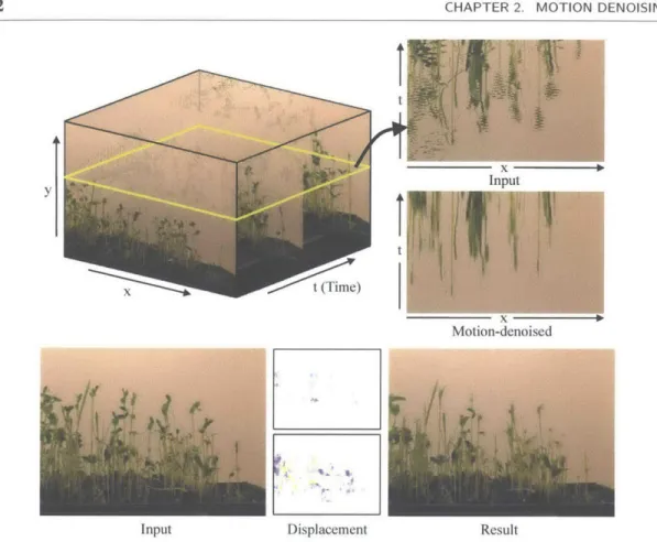
2.1 A time-lapse video of plants growing (sprouts). XT slices of the video volumes are shown for the input sequence and for the result of our motion denoising al-gorithm (top right). The motion-denoised sequence is generated by spatiotem-poral rearrangement of the pixels in the input sequence (bottom center; spatial and temporal displacement on top and bottom, respectively, following the color coding in Figure 2.5). Our algorithm solves for a displacement field that main-tains the long-term events in the video while removing the short-term, noisy motions. The full sequence and result are available in the accompanying material. 32

2.2 The responses of different temporal filters on a canonical, 1 D signal. The mean and median temporal filters operate by sliding a window temporally at each spatial location, and setting the intensity at the center pixel in the window to the mean and median intensity value of the pixels inside the window, respectively. The motion-compensated filter computes the mean intensity value along the estimated motion trajectory. In this example, the temporal filters are of size 3, centered at the pixel, and the motion denoising algorithm uses a 3 x 3 support. For illustration, we assume the temporal trajectory estimated by the motion-compensated filter is accurate until t = 6. That is, the motion from (x, t) =

(2, 6) to (4, 7) was not detected correctly. . . . . 34

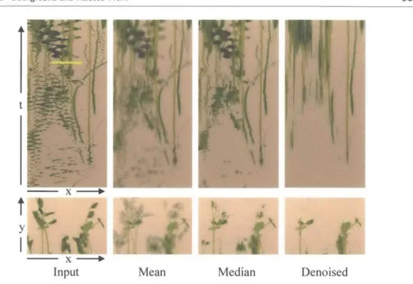
2.3 Comparison of motion denoising with simple temporal filtering on the plants sequence of Figure 2.1. At the top, zoom-ins on the left part of the XT slice from Figure 2.1 are shown for the original sequence, the (temporally) mean-filtered sequence, the median-mean-filtered sequence, and the motion-denoised se-quence. At the bottom, a representative spatial patch from each sequence is shown, taken from a region roughly marked by the yellow bar on the input video slice. . . . . 35

2.4 An illustration of the graphical model corresponding to Equation 2.5. Note that each node contains the three (unknown) components of the spatiotemporal displacement at that location. . . . . 39

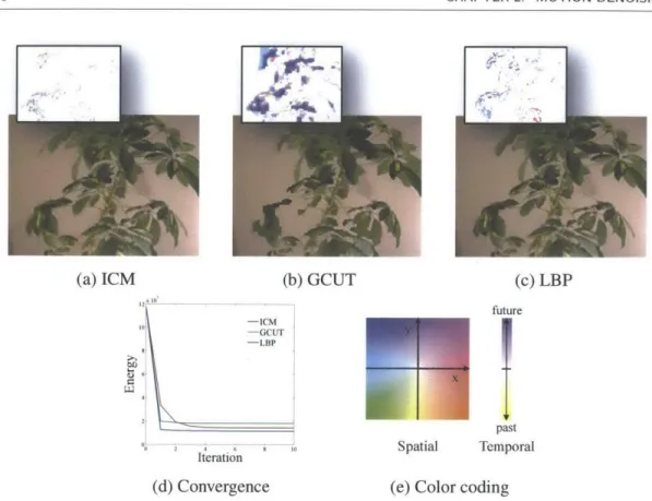
2.5 Comparison between different optimization techniques for solving Equation 2.5, demonstrated on the plant time-lapse sequence (Figure 2.7). (a-c) Representa-tive frames from each result. The spatial components of the displacement fields (overlaid) illustrate that different local minima are attained by the different op-timization methods (the full sequences are available in the accompanying ma-terial). (d) The energy convergence pattern over 10 iterations of the algorithms. (e) The color coding used for visualizing the displacement fields, borrowed from [3]. . . . . 40

2.6 A visualization of the beliefs computed by LBP for a single pixel in the plant sequence, using a 31 x 31 x 3 support. The support frame containing the pixel is zoomed-in on the upper left. The beliefs over the support are shown on the upper right, colored from blue (low energy) to red (high energy). We seek the displacement that has the minimal energy within the support region. At the bottom, the belief surface is shown for the middle frame of the support region,

clearly showing multiple equivalent (or nearly equivalent) solutions. . . . . 43

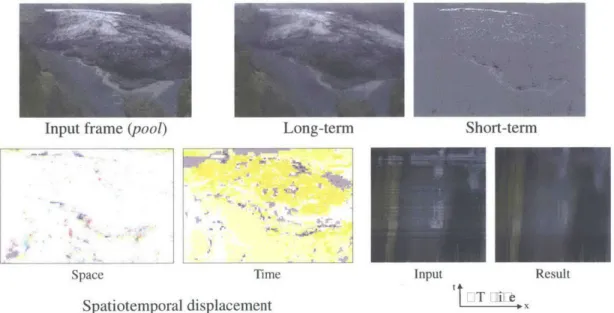
2.7 Motion denoising results on the time-lapse sequences plant and sprouts. For each sequence, we show a representative source frame (top left), representative frames of the long-term (motion-denoised) and short-term changes (top right), the computed displacement field (bottom left; spatial displacement on the left, temporal displacement on the right), and a part of an XT slice of the video vol-umes for the input and motion-denoised result (bottom right). The short-term result is computed by thresholding the color difference between the input and motion-denoised frames and copying pixels from the input. The vertical posi-tion of the spatiotemporal slice is chosen such that salient sequence dynamics are portrayed. . . . . 45

2.8 Additional results on the time-lapse sequences street, pool, and pond, shown in the same layout as in Figure 2.7. . . . . 47 2.9 Four frames from the glacier time-lapse (top), taken within the same week of

May 18, 2007, demonstrate the large variability in lighting and weather condi-tions, typical to an outdoor time-lapse footage. For this sequence, we first apply a non-uniform sampling procedure (bottom; see text) to prevent noisy frames from affecting the synthesis. The x-axis is the frame number, and the vertical lines represent the chosen frames. . . . . 48 2.10 Result on the time-lapse sequence glacier, shown in the same layout as in

Fig-ure 2.7. . . . . 48 2.11 Zoom-in on the rightmost plant in the sprouts sequence in four consecutive

frames shows that enlarging the search volume used by the algorithm can greatly improve the results. "Large support" corresponds to a 31 x 31 x 5 search vol-ume, while "small support" is the 7 x 7 x 5 volume we used in our experiments. 49

15

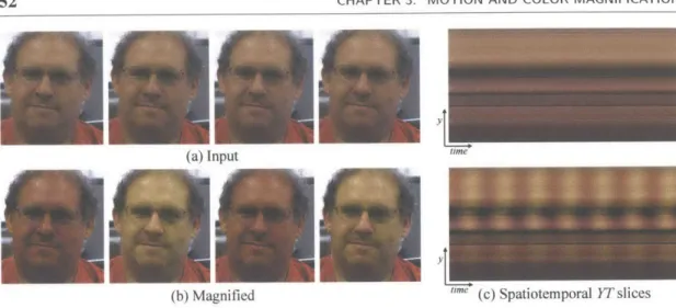
3.1 An example of using our Eulerian Video Magnification framework for visualiz-ing the human pulse. (a) Four frames from the original video sequence (face). (b) The same four frames with the subject's pulse signal amplified. (c) A verti-cal scan line from the input (top) and output (bottom) videos plotted over time shows how our method amplifies the periodic color variation. In the input se-quence the signal is imperceptible, but in the magnified sese-quence the variation is clear. The complete sequence is available in the supplemental video. . . . . . 52

3.2 Overview of the Eulerian video magnification framework. The system first de-composes the input video sequence into different spatial frequency bands, and applies the same temporal filter to all bands. The filtered spatial bands are then amplified by a given factor a, added back to the original signal, and collapsed to generate the output video. The choice of temporal filter and amplification factors can be tuned to support different applications. For example, we use the system to reveal unseen motions of a Digital SLR camera, caused by the flip-ping mirror during a photo burst (camera; full sequences are available in the supplem ental video). . . . . 56

3.3 Temporal filtering can approximate spatial translation. This effect is demon-strated here on a ID signal, but equally applies to 2D. The input signal is shown at two time instants: I(x, t) = f(x) at time t and I(x, t

+1)

t + 1. The first-order Taylor series expansion of I(x, t + 1) about x

approxi-mates well the translated signal. The temporal bandpass is amplified and added to the original signal to generate a larger translation. In this example a = 1, magnifying the motion by 100%, and the temporal filter is a finite difference filter, subtracting the two curves. . . . . 59

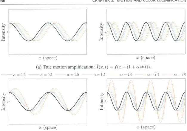
3.4 Illustration of motion amplification on a 1 D signal for different spatial frequen-cies and a values. For the images on the left side, A = 27r and 6(1) = is the true translation. For the images on the right side, A = 7r and 6(1) = . (a) The true displacement of I(x, 0) by (1 + a)6(t) at time t = 1, colored from blue (small amplification factor) to red (high amplification factor). (b) The amplified displacement produced by our filter, with colors corresponding to the correctly shifted signals in (a). Referencing Equation 3.14, the red (far right) curves of each plot correspond to (1 + a)6(t) = for the left plot, and (1 + a)6(t) = for the right plot, showing the mild, then severe, artifacts introduced in the mo-tion magnificamo-tion from exceeding the bound on (1 + a) by factors of 2 and 4, respectively. . . . . 60

3.5 Motion magnification error, computed as the L1-norm between the true motion-amplified signal (Figure 3.4(a)) and the temporally-filtered result (Figure 3.4(b)), as function of wavelength, for different values of 6(t) (a) and a (b). In (a), we fix a = 1, and in (b), 6(t) = 2. The markers on each curve represent the derived cutoff point (1 + a)6(t) = (Equation 3.14) . . . . 61 3.6 Amplification factor, a, as function of spatial wavelength A, for amplifying

motion. The amplification factor is fixed to a for spatial bands that are within our derived bound (Equation 3.14), and is attenuated linearly for higher spatial frequencies. . . . . 6 1 3.7 Spatial frequencies of the Laplacian pyramid. To estimate the spatial

frequen-cies at each pyramid level, we decompose an impulse image (a) to its spa-tial frequency bands (b), and compute the DCT coefficients for each band (c). We estimate the spatial frequency for each band (given below the DCT coeffi-cients in (c)) as the average magnitude of its corresponding DCT coefficoeffi-cients, weighted by their distance from the origin (upper left corner in (c)). . . . . 62 3.8 Heart rate extraction. (a) The spatially-averaged, temporally-bandpassed signal

from one point on the face in the face video from Figure 3.1, with the local maxima marked, indicating the pulse onsets. (b) Pulse locations used to esti-mate the pulse signal and heart rate. Each row on the y-axis corresponds to a different point on the face in no particular ordering. White pixels represent the detected peak locations at each point, and the red vertical lines correspond to the final estimated pulse locations that we use to compute the heart rate. . . . . 63

17 LIS-r OF FIGURES

3.9 Eulerian video magnification used to amplify subtle motions of blood vessels arising from blood flow. For this video, we tuned the temporal filter to a fre-quency band that includes the heart rate-0.88 Hz (53 bpm)-and set the am-plification factor to a = 10. To reduce motion magnification of irrelevant objects, we applied a user-given mask to amplify the area near the wrist only. Movement of the radial and ulnar arteries can barely be seen in the input video (a) taken with a standard point-and-shoot camera, but is significantly more no-ticeable in the motion-magnified output (b). The motion of the pulsing arteries is more visible when observing a spatio-temporal YT slice of the wrist (a) and (b). The full wrist sequence can be found in the supplemental video. . . . . 65 3.10 Temporal filters used in the thesis. The ideal filters (a) and (b) are implemented

using DCT. The Butterworth filter (c) is used to convert a user-specified fre-quency band to a second-order IIR structure that can be used for real-time pro-cessing (Section 3.4). The second-order IIR filter (d) also allows user input. These second-order filters have a broader passband than an ideal filter. . . . . . 66 3.11 Selective motion amplification on a synthetic sequence (sim4 on left). The

video sequence contains blobs oscillating at different temporal frequencies as shown on the input frame. We apply our method using an ideal temporal band-pass filter of 1-3 Hz to amplify only the motions occurring within the specified passband. In (b), we show the spatio-temporal slices from the resulting video which show the different temporal frequencies and the amplified motion of the blob oscillating at 2 Hz. We note that the space-time processing is applied uniformly to all the pixels. The full sequence and result can be found in the supplem ental video. . . . . 67 3.12 Selective motion amplification on a natural video (guitar). Each of the guitar's

strings (a) vibrates at different frequency. (b-c) The signals of intensities over time (top) and their corresponding power spectra (bottom) are shown for two pixels located on the low E and A strings, respectively, superimposed on the representative frame in (a). The power spectra clearly reveal the vibration fre-quency of each string. Using an appropriate temporal bandpass filter, we are able to amplify the motion of particular strings while maintaining the motion of the others. The result is available in the supplemental video. . . . . 68

LIST OF FIGURES 18

3.13 Proper spatial pooling is imperative for revealing the signal of interest. (a) A frame from the face video (Figure 3.1) with white Gaussian noise added

(a = 0.1). On the right are intensity traces over time for the pixel marked

blue on the input frame, where (b) shows the trace obtained when the (noisy) sequence is processed with the same spatial filter used to process the original

face sequence, a separable binomial filter of size 20, and (c) shows the trace

when using a filter tuned according to the estimated radius in Equation 3.16, a binomial filter of size 80. The pulse signal is not visible in (b), as the noise level is higher than the power of the signal, while in (c) the pulse is clearly visible (the periodic peaks about one second apart in the trace). . . . . 71

3.14 Comparison between Eulerian and Lagrangian motion magnification on a syn-thetic sequence with additive noise (a). (b) The minimal error, min(EE, EL),

computed as the (frame-wise) RMSE between each method's result and the true motion-magnified sequence, as function of noise and amplification, col-ored from blue (small error) to red (large error), with (left) and without (right) spatial regularization in the Lagrangian method. The black curves mark the intersection between the error surfaces, and the overlayed text indicate the best performing method in each region. (c) RMSE of the two approaches as func-tion of noise (left) and amplificafunc-tion (right). (d) Same as (c), using spatial noise on ly. . . . . 7 3

3.15 Motion magnification of a crane imperceptibly swaying in the wind. (a) Top: a zoom-in onto a patch in the original sequence (crane) shown on the left. Bot-tom: a spatiotemporal XT slice of the video along the profile marked on the zoomed-in patch. (b-c) Linear (Section 3.2) and phase-based motion magnifi-cation results, respectively, shown for the corresponding patch and spatiotem-poral slice as in (a). The previous, linear method visualizes the crane's motion, but amplifies both signal and noise and introduces artifacts for higher spatial frequencies and larger motions, shown by the clipped intensities (bright pixels) in (b). In comparison, our new phase-based method supports larger magni-fication factors with significantly fewer artifacts and less noise (c). The full sequences are available in the supplemental video . . . . 75

19 LIST OF FIGURES

LIST OF FIGURES 3.16 Our phase-based approach manipulates motion in videos by analyzing the

sig-nals of local phase over time in different spatial scales and orientations. We use complex steerable pyramids to decompose the video and separate the amplitude of the local wavelets from their phase (a). We then temporally filter the phases independently at at each location, orientation and scale (b). Optionally, we ap-ply amplitude-weighted spatial smoothing (c, Sect. 3.3.6) to increase the phase SNR, which we empirically found to improve the results. We then amplify or attenuate the temporally-bandpassed phases (d), and reconstruct the video (e). This example shows the processing pipeline for the membrane sequence (Sect. 3.3.7), using a pyramid of two scales and two orientations (the relative difference in size between the pyramid levels is smaller in this figure for clarity of the visualization). . . . . 76

3.17 Phase-based motion magnification is perfect for sinusoidal functions. In these plots, the initial displacement is 6(t) = 1. While the errors for the linear tech-nique (Section 3.2) are dependent on wavelength for sinusoids, there is no such dependence for the present technique and the error is uniformly small. The vertical axis in (d) is logarithmic. . . . . 78

3.18 A comparison between octave and sub-octave bandwidth pyramids for motion magnification. Each color in the idealized frequency response represents a dif-ferent filter. (a) The original steerable pyramid of Portilla and Simoncelli [37]. This pyramid has octave bandwidth filters and four orientations. The impulse response of the filters is narrow (rows 2 - 3), which reduces the maximum magnification possible (rows 4 - 5). (b-c) Pyramid representations with two and four filters per octave, respectively. These representations are more over-complete, but support larger magnification factors . . . . 80

3.19 For general non-periodic structures, we achieve performance at least four times that of the linear technique, and do not suffer from clipping artifacts (a). For large amplification, the different frequency bands break up due to the higher bands having a smaller window (b). . . . . 82 20

3.20 The impulse response of the steerable filter bank illustrates the artifacts that arise when modulating phase to magnify motion. (a) The impulse response of a wavelet being phase shifted. As the phase increases (orange corresponds to 3),

the primary peak shifts to the right decreasing under the Gaussian window. A secondary peak forms to the left of the primary peak. (c) Error in magnification of the impulse response as the impulse is moved under the Gaussian window. The maximum (normalized) error occurs when the phase-shifted wavelet no longer overlaps with the true-shifted one. The constant C = o- is marked on the

curve. ... ... 83

3.21 Comparison between linear and phase-based Eulerian motion magnification in handling noise. (a) A frame in a sequence of IID noise. In both (b) and (c), the motion is amplified by a factor of 50, where (b) uses the linear technique (Section 3.2) and (c) uses the phase-based approach. (d) shows a plot of the error as function of noise for each method, using several magnification factors. 84

3.22 Over-completeness as function of the bound on the amplification factor, 0Z, in our pyramid representation with different number of orientations, k, 1-6 filters per octave (points left to right), and assumed motion 6(t) = 0.1 pixels. For example, a half-octave, 8-orientation pyramid is 32x over-complete, and can amplify motions up to a factor of 20, while a similar quarter-octave pyramid can amplify motions by a factor of 30, and is 43x over-complete. . . . . 86

3.23 Comparison of the phabased motion magnification result on the camera se-quence (d) with the result of linear motion magnification (a), denoised by two state-of-the-art video denoising algorithms: VBM3D [1 1] (b) and motion-based denoising by Liu and Freeman [24] (c). The denoising algorithms cannot deal with the medium frequency noise, and are computationally intensive. The full videos and similar comparisons on other sequences are available in the supple-m entary supple-m aterial. . . . . 90

21 LIST OF FIGURES

3.24 A controlled motion magnification experiment to verify our framework. (a) A hammer strikes a metal structures which then moves with a damped oscilla-tory motion. (b) A sequence with oscillaoscilla-tory motion of amplitude 0.1 pixels is magnified 50 times using our algorithm and compared to a sequence with oscil-latory motion of amplitude 5 pixels (50 times the amplitude). (c) A comparison of acceleration extracted from the video with the accelerometer recording. (d) The error in the motion signal we extract from the video, measured as in (c), as function of the impact force. Our motion signal is more accurate as the motions in the scene get larger. All videos are available in the supplementary material. . 91

3.25 Motion attenuation stabilizes unwanted head motions that would otherwise be exaggerated by color amplification. The exaggerated motions appear as wiggles in the middle spatiotemporal slice on the right, and do not appear in the bottom right slice. The full sequence is available in the supplemental video. . . . . 92

3.26 Motion magnification can cause artifacts (cyan insets and spatiotemporal times-lices) in regions of large motion such as those in this sequence of a boy jumping on a platform (a). We can automatically remove such artifacts by identifying regions where the phase change exceeds our bound or a user-specified threshold (b). When the boy hits the platform, the time slice (purple highlights) shows that the subtle motions of the platform or the camera tripod due to the boy's jump are magnified in both cases . . . . 94

3.27 A real-time computational "microscope" for small visual changes. This snap-shot was taken while using the application to visualize artery pulsation in a wrist. The application was running on a standard laptop using a video feed from an off-the-shelf webcam. A demo is available on the thesis webpage. . . . 95

3.28 An interface that allows the user to sweep through the temporal frequency do-main and examine temporal phenomena in a simple and intuitive manner. A demo is available in the accompanying video. . . . . 96

LIST OF FIGURES 23

3.29 A visualization of the dominant temporal frequencies for two sequences: face (left; representative frame on the left, visualization on the right) and guitar (right; frame at the top, visualization at the bottom), produced by showing, at every pixel, the frequency of maximum energy in the temporal signal recorded at the pixel. This visualization clearly shows the pulsatile areas of the face from which a reliable pulse signal can be extracted, and the frequencies in which the different strings of the guitar vibrate. . . . . 97

List of Tables

3.1 Table of a, AC, W, Wh values used to produce the various output videos. For

face2,

f,

motion magnification. The representation size is given as a factor of the original frame size, where k represents the number of orientation bands and n represents the number of filters per octave for each orientation. . . . . 88 C. 1 Videos used in Chapter 3 and their properties. All the videos and results are

available through the thesis web page. . . . .111

Chapter 1

Introduction

The only reason for time is so that everything doesn't happen at once.

-Albert Einstein

Modem photography provides us with useful tools to capture physical phenomena occur-ring over different scales of time (Figure 1. 1). At one end of the spectrum, high-speed imagery now supports frame rates of 6 MHz (6 million frames per second), allowing the high quality capture of ultrafast events such as shock waves and neural activity [20]. At the other end of the spectrum, time-lapse sequences can reveal long-term processes spanning decades, such as the evolution of cities, melting of glaciers, and deforestation, and have even recently become available on a planetary scale [12]. However, methods to automatically identify and analyze physical processes or trends in visual data are still in their infancy [17]

This thesis is comprised of several projects I explored during my PhD, which focus on ana-lyzing and manipulating temporal variations in video and image sequences, in order to facilitate the analysis of temporal phenomena captured by imagery, and reveal interesting temporal sig-nals and processes that may not be easily visible in the original data. Here we give a high-level overview of these projects. The details of the proposed techniques and review of related lit-erature are given in the chapters to follow. In the rest of the thesis, I will refer to changes in intensities recorded in video and images over time (caused by change in color, or motion) as "temporal variation", or simply "variation" for brevity.

Removing distracting variation. First, we explored the problem of removing motions and changes that distract from the main temporal signals of interest. This is especially useful for time-lapse sequences that are often used for long-period medical and scientific analysis, where dynamic scenes are captured over long periods of time. When day- or even year-long events are condensed into minutes or seconds, the pixels can be temporally inconsistent due to the

significant time aliasing. Such aliasing effects take the form of objects suddenly appearing and disappearing, or illumination changing rapidly between consecutive frames, making the long-term processes in those sequences difficult to view or further analyze. For example, we can more easily measure the growth of outdoor plants by re-synthesizing the video to suppress the leaves waving in the wind.

We designed a video processing system which treats short-term visual changes as noise, long-term changes as signal, and re-renders a video to reveal the underlying long-term events [44] (Chapter 2). We call this technique "motion denoising" in analogy to image denoising (the process of removing sensor noise added during image capture). The result is an automatic decomposition of the original video into short- and long-term motion components. We show that naive temporal filtering approaches are often incapable of achieving this task, and present a novel computational approach to denoise motion without explicit motion analysis, making it applicable to diverse videos containing highly involved dynamics common to long-term im-agery.

Magnifying imperceptible variation. In other cases, one may want to magnify motions and changes that are too subtle to be seen by the naked eye. For example, human skin color varies slightly with blood circulation (Figure 3.1). This variation, while invisible to the naked eye, can

3 Chapter 2

Milliseconds Seconds, Minutes Months, years

104 fps (high-speed) 101 fps (standard videos) 10- fps (time-lapse)

Figure 1.1: Timescales in imagery. High-speed videos (left) capture short-term, fast motions, such as vibration of engines and small eye movements. Normal-rate videos (middle) can capture physiological functions, such as heart rate and respiratory motions. Time-lapse sequences (right) depict long-term physical processes, such as the growth of plants and melting of glaciers. The listed frame rates (Frames Per Second; fps) are only representative rates and can vary considerably between videos in each category.

29

be exploited to extract pulse rate and reveal spatial blood flow patterns. Similarly, motion with low spatial amplitude, while hard or impossible for humans to see, can be magnified to reveal interesting mechanical behavior.

We proposed efficient methods that combine spatial and temporal processing to emphasize subtle temporal changes in videos [59, 45, 55] (Chapter 3). These methods use an Eulerian specification of the changes in the scene, analyzing and amplifying the variation over time at fixed locations in space (pixels). The first method we proposed, which we call the linear

method, takes a standard video sequence as input, and applies spatial decomposition followed

by temporal filtering to the frames. The resulting temporal signal is then amplified to reveal hid-den information (Section 3.2). This temporal filtering approach can also reveal low-amplitude spatial motion, and we provide a mathematical analysis that explains how the temporal intensity signal interplays with spatial motion in videos, which relies on a linear approximation related to the brightness constancy assumption used in traditional optical flow formulations. This ap-proximation (and thus the method) only applies to very small motions, but those are exactly the type of motions we want to amplify.

The linear method to amplify motions is simple and fast, but suffers from two main draw-backs. Namely, noise gets amplified linearly with the amplification, and the approximation to the amplified motion breaks down quickly for high spatial frequencies and large motions. To counter these issues, we proposed a better approach to process small motions in videos, where we replace the linear approximation with a localized Fourier decomposition using complex-valued image pyramids [55] (Section 3.3). The phase variations of the coefficients of these pyramids over time correspond to motion, and can be temporally processed and modified to manipulate the motion. In comparison to the linear method, this phase-based technique has a higher computational overhead, but can support larger amplification of the motion with fewer artifacts and less noise. This further extends the regime of low-amplitude physical phenomena that can be analyzed and visualized by Eulerian approaches.

Visualization. We produced visualizations that suppress or highlight different patterns of tem-poral variation by synthesizing videos with smaller or larger changes (Chapters 2, 3). For small-amplitude variations, we also explored interactive user interfaces and visualization tools to assist the user in exploring temporal signals in videos (Section 3.4). We built a prototype ap-plication that can amplify and reveal micro changes from video streams in real-time and show phenomena occurring at temporal frequencies selected by the user. This application can run

30 CHAPTER 1. INTRODUCTION on modem laptops and tablets, essentially turning those devices into "microscopes" for minus-cule visual changes. We can also produce static image visualizations summarizing the temporal frequency content in a video.

This thesis is largely based on work that appeared previously in the 2011 IEEE Conference on Computer Vision and Pattern Recognition (CVPR) [44], and ACM Transactions on Graph-ics (Proceedings SIGGRAPH 2012 and 2013) [59, 55]. All the the accompanying materials referenced here, including illustrative supplementary videos, software, the video sequences we experimented with, and our results, can be conveniently accessed though the thesis web page:

Chapter 2

Motion Denoising

Motions can occur over both short and long time scales. In this chapter, we introduce motion

denoising, a video processing technique that treats short-term visual changes as noise,

long-term changes as signal, and re-renders a video to reveal the underlying long-long-term events. We demonstrate motion denoising for time-lapse videos. One of the characteristics of traditional time-lapse imagery is stylized jerkiness, where short-term changes in the scene appear as small and annoying jitters in the video, often obfuscating the underlying temporal events of inter-est. We apply motion denoising for resynthesizing time-lapse videos showing the long-term evolution of a scene with jerky short-term changes removed. We show that existing filtering ap-proaches are often incapable of achieving this task, and present a novel computational approach to denoise motion without explicit motion analysis. We demonstrate promising experimental results on a set of challenging time-lapse sequences.

* 2.1 Introduction

Randomness appears almost everywhere in the visual world. During the imaging process, for example, randomness occurs in capturing the brightness of the light going into a camera. As a result, we often see noise in images captured by CCD cameras. As image noise is mostly unwanted, a large number of noise removal approaches have been developed to recover the underlying signal in the presence of noise.

Randomness also appears in the form of motion. Plants sprout from soil in an unplanned order; leaves move arbitrarily under wind; clouds spread and gather; the surface of our planet changes over seasons with spotted decorations of snow, rivers, and flowers.

As much as image noise is often unwanted, motion randomness can also be undesired. For example, traditional time-lapse sequences are often characterized by small and annoying jitters

32 CHAPTER 2. MOTION DENOISING

Y Input

t

Motion-denoised

Input Displacement Result

Figure 2.1: A time-lapse video of plants growing (sprouts). XT slices of the video volumes are shown

for the input sequence and for the result of our motion denoising algorithm (top right). The motion-denoised sequence is generated by spatiotemporal rearrangement of the pixels in the input sequence (bottom center; spatial and temporal displacement on top and bottom, respectively, following the color coding in Figure 2.5). Our algorithm solves for a displacement field that maintains the long-term events in the video while removing the short-term, noisy motions. The full sequence and result are available in the accompanying material.

resulting from short-term changes in shape, lighting, viewpoint, and object position, which obfuscate the underlying long-term events depicted in a scene. Atmospheric and heat turbulence often show up as short-term, small and irregular motions in videos of far-away scenes.

It is therefore important to remove random, temporally inconsistent motion. We want to design a video processing system that removes temporal jitters and inconsistencies in an input video, and generate a temporally smooth video as if randomness never appeared. We call this technique motion denoising in analogy to image denoising. Since visual events are decomposed

Sec. 2.2. Background and Related Work 33

into slow-varying and fast-changing components in motion denoising, such technique can be useful for time-lapse photography, which is widely used in the movie industry, especially for documentary movies, but has recently become prevalent among personal users as well. It can also assist long-period medical and scientific analysis. For the rest of the chapter we will refer to motion denoising and its induced motion decomposition interchangeably.

Motion denoising is by no means a trivial problem. Previous work on motion editing has focused on accurately measuring the underlying motion and carefully constructing coherent motion layers in the scene. These kind of motion-based techniques are often not suitable for analyzing time-lapse videos. The jerky nature of these sequences violates the core assumptions of motion analysis and optical flow, and prevents even the most sophisticated motion estimation algorithm from obtaining accurate enough motion for further analysis.

We propose a novel computational approach to motion denoising in videos that does not require explicit motion estimation and modeling. We formulate the problem in a Bayesian framework, where the goal is to recover a "smooth version" of the input video by reshuffling its pixels spatiotemporally. This translates to a well-defined inference problem over a 3D Markov Random Field (MRF), which we solve using a time-space optimized Loopy Belief Propagation (LBP) algorithm. We show how motion denoising can be used to eliminate short-term motion jitters in time-lapse videos, and present results for time-lapse sequences of different nature and

scenes.

* 2.2 Background and Related Work

The input to our system is an M x N x T video sequence, I(x, y, t), with RGB intensities

given in range [0, 255]. Our goal is to produce an M x N x T output sequence, J(x, y, t), in which short-term jittery motions are removed and long-term scene changes are maintained. A number of attempts have been made to tackle similar problems from a variety of perspectives, which we will now briefly review.

Temporal filtering. A straightforward approach is to pass the sequence through a temporal low-pass filter

J(x, y, t) = f (I(x, y, {k}t"') (2.1) where

f

f

CHAPTER 2. MOTION DENOISING A7 6 5 t 4 3 2 1 2 3 4 5 - x

-Original Mean Median Motion-

Motion-signal compensated denoised

Figure 2.2: The responses of different temporal filters on a canonical, ID signal. The mean and median

temporal filters operate by sliding a window temporally at each spatial location, and setting the intensity at the center pixel in the window to the mean and median intensity value of the pixels inside the window, respectively. The motion-compensated filter computes the mean intensity value along the estimated motion trajectory. In this example, the temporal filters are of size 3, centered at the pixel, and the motion denoising algorithm uses a 3 x 3 support. For illustration, we assume the temporal trajectory estimated

by the motion-compensated filter is accurate until t = 6. That is, the motion from (x, t) = (2, 6) to

(4, 7) was not detected correctly.

simple and fast, has an obvious limitation - the filtering is performed independently at each pixel. In a dynamic scene with rapid motion, pixels belonging to different objects are averaged, resulting in a blurred or discontinuous result. Figure 2.2 demonstrates this on a canonical signal, and figure 2.3 further illustrates these effects on a natural time-lapse video.

To address this issue, motion-compensated filtering was introduced, filtering the sequence along motion trajectories (e.g., [34]). Such techniques are commonly employed for video com-pression, predictive coding, and noise removal. Although this approach is able to deal with some of the blur and discontinuity artifacts, as pixels are only integrated along the estimated motion path, it does not filter the actual motion (i.e. making the motion trajectory smoother), but rather takes the motion into account for filtering the sequence. In addition, errors in the motion estimation may result in unwanted artifacts at object boundaries.

Motion editing. One work that took a direct approach to motion editing in videos is "Motion Magnification" [23]. A layer segmentation system was proposed for exaggerating motions that might otherwise be difficult or even impossible to notice. Similar to our work, they also manipulate video data to resynthesize a sequence with modified motions. However, our work modifies the motion without explicit motion analysis or layer modeling that are required by

Sec. 2.2. Background and Related Work

II

t

y.

x

Input Mean Median Denoised

Figure 2.3: Comparison of motion denoising with simple temporal filtering on the plants sequence of Figure 2.1. At the top, zoom-ins on the left part of the XT slice from Figure 2.1 are shown for the original sequence, the (temporally) mean-filtered sequence, the median-filtered sequence, and the motion-denoised sequence. At the bottom, a representative spatial patch from each sequence is shown,

taken from a region roughly marked by the yellow bar on the input video slice.

their method. In fact, layer estimation can be challenging for the sequences we are interested in; these sequences may contain too many layers (e.g., leaves) for which even state-of-the-art layer segmentation algorithms would have difficulties producing reliable estimates.

Motion denoising has been addressed before in a global manner, known as video stabiliza-tion (e.g., [31, 28]). Camera jitter (mostly from hand-held devices) is modeled using image-level transforms between consecutive frames, which are used to synthesize a sequence with smoother camera motion. Image and video inpainting techniques are often utilized to fill-in missing content in the stabilized sequence. In contrast, we focus on stabilization at the object

level, supporting spatially-varying, pixel-wise displacement within a single frame. Inpainting

is built-in naturally into our formulation.

Time-lapse videos. Time-lapse videos are valuable for portraying events occurring through-out long time periods. Typically, a frame is captured once every few minutes or hours over a

CHAPTER 2. MOTION DENOISING

long time period (e.g., weeks, months), and the captured frames are then stacked in time to cre-ate a video depicting some long-term phenomena [10]. Captured sequences span a large variety of scenes, from building construction, through changes in the human body (e.g., pregnancy, aging), to natural phenomena such as celestial motion and season change. Capturing time-lapse sequences no longer requires an expert photographer. In fact, it is supported as built-in functionality in many modem consumer digital cameras.

Although sequences captured by time-lapse photography are very different in nature, they all typically share a common artifact-stylized jerkiness-caused by temporal aliasing that is inherent to the time-lapse capture process. Rapidly moving objects, as well as lighting changes, and even small camera movements (common if the camera is positioned outdoors) then appear as distracting, non-physical jumps in the video. These effects might sometimes be desirable, however in often cases they simply clutter the main temporal events the photographer wishes to portray.

Previous academic work involving time-lapse sequences use them as an efficient represen-tation for video summarization. Work such as [4, 39] take a video-rate footage as input, and output a sequence of frames that succinctly depict temporal events in the video. Work such as [39, 40] can take an input time-lapse video, and produce a single-frame representation of that sequence, utilizing information from throughout the time span. Time-lapse sequences have also been used for other applications. For example, Weiss [57] uses a sequence of images of a scene under varying illumination to estimate intrinsic images. These techniques and applications are significantly different from ours. Both input and output of our system are time-lapse videos, and our goal is to improve the input sequence quality by suppressing short-term distracting events and maintaining the underlying long-term flux of the scene.

Direct editing of time-lapse imagery was proposed in [49] by factorizing each pixel in an input time-lapse video into shadow, illumination and reflectance components, which can be used for relighting or editing the sequence, and for recovering the scene geometry. In our work, we are interested in a different type of decomposition: separating a time-lapse sequence into shorter- and longer-term events. These two types of decompositions can be complimentary to each other.

Geometric rearrangement. In the core of our method is a statistical (data-driven) algorithm for inferring smooth motion from noisy motion by rearranging the input video. Content rear-rangement in images and video has been used in the past for various editing applications. Image 36

reshuffling is discussed in [9]. They work in patch space, and the patch moves are constrained to an underlying coarse grid which does support relatively small motions common to time-lapse videos. We, on the other hand, work in pixel resolution, supporting both small and irregular displacements. [38] perform geometric image rearrangement for various image editing tasks using a MRF formulation. Our work concentrates on a different problem and requires different formulation. Inference in videos is much more challenging than in images, and we use different inference tools from the ones used in their work.

For videos, [46] consider the sequence appearance and dynamics for shifting entire frames to create a modified playback. [39] generate short summaries for browsing and indexing surveillance data by shifting individual pixels temporally while keeping their spatial locations intact. [52] align two videos using affine spatial and temporal warps. Our problem is again very different from all these work. Temporal shifts alone are insufficient to denoise noisy motion, and spatial offsets must be defined in higher granularity than the global frame or video. This makes the problem much more challenging to solve.

M 2.3 Formulation

We model the world as evolving slowly through time. That is, within any relatively small time span, we assume objects in the scene attain some stable configuration, and changes to these configurations occur in low time rates. Moreover, we wish to make use of the large redun-dancy in images and videos to infer those stable configurations. This leads to the following formulation.

Given an input video I, we seek an output video J that minimizes the energy E(J), defined as

E(J) = J(x, y, t) - I(x, y, t)

I

x'y't X'y't

subject to

J(X, y, t) I(x + wX(X, y, t), y + wy (X, y, t), t + Wt (X, y, t)) (2.3) for spatiotemporal displacement field

w(x, y, t) E {(6, 6y, 6t) : 6X < As, 16Y| 1 AS, A I At}, (2.4) where (A8, At) are parameters defining the support (search) region.

37

CHAPTER 2. MOTION DENOISING In this objective function, the first term is a fidelity term, enforcing the output sequence to resemble the input sequence at each location and time. The second term is a temporal coherence term, which requires the solution to be temporally smooth. The tension between those two terms creates a solution which maintains the general appearance of the input sequence, and is temporally smooth. This tradeoff between appearance and temporal coherence is controlled via the parameter a.

As J is uniquely defined by the spatiotemporal displacements, we can equivalently rewrite Equation 2.2 as an optimization on the displacement field w. Further parameterizing p =

(x, y, t), and plugging constraint 2.3 into Equation 2.2, we get

E(w ) = I:1 (p + w(p)) - I(p)|I+

a I(p + w(p))- I(r + (r)) 12 +

p,r cAt (p)

y E Apq w(p) - w(q) , (2.5)

p,qeGA(p)

where we added an additional term for regularizing the displacement field w, with weight

Apq = exp-1 I(p) - I(q) 12}. 0 is learnt as described in [50]. Apq assigns varying weight to discontinuities in the displacement map, as function of the similarity between neighboring pixels in the original video. K(p) denotes the spatiotemporal neighborhood of pixel p, and

Ms (p), At (p) C .A(p) denote the spatial and temporal neighbors of p, respectively. We use the six spatiotemporal pixels directly connected to p as the neighborhood system.

a and -y weight the temporal coherence and regularization terms, respectively. The L₂

norm is used for temporal coherence to discourage motion discontinuities, while L1 is used in

the fidelity and regularization terms to remove noise from the input sequence, and to account for discontinuities in the displacement field, respectively.

E

2.3.1 Optimization

We optimize Equation 2.5 discretely on a 3D MRF corresponding to the three-dimensional video volume, where each node p corresponds to a pixel in the video sequence and represents the latent variables w(p). The state space in our model is the set of possible three-dimensional displacements within a predefined search region (Equation 2.4). The potential functions are 38

Sec. 2.3. Formulation 39

o

=

Figure 2.4: An illustration of the graphical model corresponding to Equation 2.5. Note that each node contains the three (unknown) components of the spatiotemporal displacement at that location.

given by

-p p(W W) =

|(P

r(w(p), w(r)) = a| I(p + w(p)) - I(r + w(r))| 12+

yAprjW(p) - W(r)1, (2.7)

',(w(p), w(q)) = -yApqIw(p) - w(q) (2.8)

where Op is the unary potential at each node, and Op4

r, /)pq denote the temporal and spatial pairwise potentials, respectively. Figure 2.4 depicts the structure of this graphical model.

We have experimented with several optimization techniques for solving Equation 2.5, namely Iterated Conditional Modes (ICM), a-expansion (GCUT) [6] and Loopy Belief Propagation (LBP) [60]. Our temporal pairwise potentials (Equation 2.7) are neither a metric nor a semi-metric, which makes the graph-cut based algorithms theoretically inapplicable to this optimiza-tion. Although previous work use those algorithms ignoring the metric constraints and still report good results (e.g., [38]), our experiments consistently showed that LBP manages to pro-duce more visually appealing sequences, and in most cases also achieves lower energy solutions compared to the other solvers. We therefore choose LBP as our inference engine.

Figure 2.5 compares the results of the three optimizations. The complete sequences are available in the supplementary material. The ICM results suffer, as expected, from noticeable 39 Sec. 2.3. Formulation

40 CHAPTER 2. MOTION DENOISING (a) 1CM (b) GCUT (c) LBP _7 future -1CM_-'CM GCUT -LBP past - -- We Spatial Temporal Iteration

(d) Convergence (e) Color coding

Figure 2.5: Comparison between different optimization techniques for solving Equation 2.5, demon-strated on the plant time-lapse sequence (Figure 2.7). (a-c) Representative frames from each result. The spatial components of the displacement fields (overlaid) illustrate that different local minima are attained by the different optimization methods (the full sequences are available in the accompanying material). (d) The energy convergence pattern over 10 iterations of the algorithms. (e) The color coding used for visualizing the displacement fields, borrowed from [3].

discontinuities. There are also noticeable artifacts in the graph-cut solution. As part of our pair-wise potentials are highly non-metric, it is probable that a-expansion will make incorrect moves that will adversely affect the results. All three methods tend to converge quickly within 3 - 5 iterations, which agrees with the related literature [50]. Although the solution energies tend to be within the same ballpark, we noticed they usually correspond to different local minima.

* 2.3.2 Implementation Details

Our underlying graphical model is a massive 3D grid, which imposes computational difficul-ties in both time and space. For tractable runtime, we extend the message update schedule by

Sec. 2.3. Formulation 41 Tappen and Freeman [51] to 3D, by first sending messages (forth and back) along rows in all frames, then along columns, and finally along time. This sequential schedule allows informa-tion to propagate quickly through the grid, and helps the algorithm converge faster. To search larger ranges, we apply LBP to a spatiotemporal video pyramid. Since time-lapse sequences are temporally aliased, we apply smoothing to the spatial domain only, and sample in the tem-poral domain. At the coarser level, the same search volume effectively covers twice the volume used in the finer level, allowing the algorithm to consider larger spatial and temporal ranges. To propagate the displacements to the finer level, we bilinear-interpolate and scale (multiply by 2) the shifts, and use them as centers of the search volume at each pixel in the finer level.

The complexity of LBP is linear in the graph size, but quadratic in the state space. In our model, we have a K3 search volume (for A, = At = K), which requires K6 computations per message update and may quickly become intractable even for relatively small search volumes. Nevertheless, we can get significant speedup in the computation of the spatial messages using distance transform, as the 3D displacement components are decoupled in the LI-norm distance. Felzenszwalb and Huttenlocher have shown that computing a distance transform on such 3D label grids can be reduced to consecutive efficient computations of 1 D distance transforms [13]. The overall complexity of this computation is 0(3K3), which is linear in the search range. For

our multiscale computation, Liu et al. [27] already showed how the distance transform can be extended to handle offsets (corresponding to the centers of the search volumes obtained from the coarser level of the video pyramid) in 2D. Following the reduction in [13] therefore shows that we can trivially handle offsets in the 3D case as well. We note that the distance transform computation is not an approximation, and results in the exact message updates.

We briefly demonstrate the computation of the spatial messages in our formulation using distance transform, and refer the interested reader to [13] for more details. Our min-sum spatial message update equation can be written as

mp_,q(wq) = min (Iwp - wgI + hp(wp)), (2.9)

Wp

We can expand Equation 2.9 as

= min (W -w+ + w - w |+ K- w + hp(wp).(.

Mi w tI+(i w qY mnJx-wJ+h~p (2.10)

Written in this form, it is evident that the the 3D distance transform can be computed by con-secutively computing the distance transform of each component in place. Note that the order of the components above was chosen arbitrarily, and does not affect the decomposition.

This yields a significant improvement in running time, since 2/3 of the messages propagat-ing through the graph can be computed in linear time. Unfortunately, we cannot follow a similar approach for the temporal messages, as the temporal pairwise potential function (Equation 2.7) is non-convex.

This massive inference problem imposes computational difficulties in terms of space as well. For example, a 5003 video sequence with a 103 search region requires memory, for the messages only, of size at least 5003 x 103 x 6 x 4 ~ 3 terabytes (!). Far beyond current available RAM, and probably beyond the average available disk space. We therefore restrict our attention to smaller sequences and search volumes. As the messages structure cannot fit entirely in memory, we store it on disk, and read and write the necessary message chunks on need. For our message update schedule, it suffices to maintain in memory the complete message structure for one frame for passing messages spatially, and two frames for passing messages temporally. This imposes no memory difficulty even for larger sequences, but comes at the cost of lower performance as disk I/O is far more expensive than memory access. Section 2.4 details the algorithm's space and time requirements for the videos and parameters we used.

Finally, once LBP converges or message passing is complete, the MAP label assignment is traditionally computed independently at each node [14]:

w7p = arg min (p (wp) + E mqp (wp)). (2.11)

qC (p)

For our problem, we observe that the local conditional densities are often multi-modal (Fig-ure 2.6), indicating multiple possible solutions that are equivalent, or close to equivalent, with respect to the objective function. The label (displacement) assigned to each pixel using Equa-tion 2.11 therefore depends on the order of traversing the labels, which is somewhat arbitrary.