2.672 experiment design : heat sink fin configurations

2.672 Experiment Design: Heat Sink Fin

Configurations

by

Zachary W. Reynolds

Submitted to the Department of Mechanical Engineering

in partial fulfillment of the requirements for the degree of

Bachelor of Science in Mechanical Engineering

at the

MASSACHUSETTS INSTITUTE OF TECHNOLOGY

June 2007

@

Massachusetts Institute of Technology 2007. All rights reserved.

Author ... ... 0

Department of Mechanical Engineering

May 11, 2007

Certified by

Douglas P. Hart

Professor of Mechanical Engineering

Thesis Supervisor

Accepted by ...

JUN

2

12007

L ARI&.

F .

John H. Lienhard V

Chairman, Undergraduate Thesis Committee

MRCHIVES

2.672 Experiment Design: Heat Sink Fin Configurations

by

Zachary W. Reynolds

Submitted to the Department of Mechanical Engineering on May 11, 2007, in partial fulfillment of the

requirements for the degree of

Bachelor of Science in Mechanical Engineering

Abstract

2.672 is an undergraduate mechanical engineering laboratory course which requires students to solve real-world problems using both theoretical calculations and labora-tory experiments. Many of the experiments currently in the laboralabora-tory have aged and their replacement presents an opportunity for the introduction of a new experiment. In this proposed experiment, students will optimize a heat sink for a certain type of rack-mount server. For a correct execution of the experiment, students will test the power dissipation of several different heat sinks against a model for how they should behave using principles of incompressible flow, extended surfaces and heat exchang-ers. An apparatus has been designed and constructed to simulate the air duct inside one possible server, and allow for measurements to be taken of power dissipation, temperature, and pressure in the duct. Seven different heat sink configurations were chosen to provide students with insight into how each parameter alters the effective-ness of the heat sink. Students are then asked to choose the parameters which give the optimal configuration.

Thesis Supervisor: Douglas P. Hart

Acknowledgments

I would first like to thank Professor Doug Hart for suggesting this project for un-dergraduate thesis work, and for providing well-needed guidance during the design process.

I also thank Bryan Ruddy, a Ph.D student in the Mechanical Engineering De-partment, for guiding the details of this project during its course. This project was Bryan's brainchild, and without him it never would have progressed from concept to design to prototype. Bryan also designed almost all of the electronics for the project and machined the heat sinks used, without which testing of the apparatus would have been nearly impossible. His guidance during the theoretical modelling of the experiment taught me more than any other class this semester.

Thanks to Dick Fenner, director of M.E. Undergraduate Teaching Labs, for pro-viding materials and advice during the initial construction of the apparatus. Dick saved me from countless hours of "doing it the dumb way."

I thank Dr. Barbara Hughey, for her help in navigating the maze of ordering parts and letting me store my apparatus in her lab.

Thanks to the staff of Pappalardo Labs: Joe Cronin, Bob Gertsen, Steve Haberek, Bob Nuttal, and Jimmy "the cab driver" Dudley for their help and patience during the machining of many of the parts for the apparatus.

Also, thanks to the members of the Bioinstrumentation Lab, for opening the door to their lab for me tens of times and for allowing me space to perform assembly and testing.

Thanks to Lydia Chilton for the use of her camera to photograph the apparatus. Lastly, I would like to thank Martin McBrien, my neighbor, for showing me what a. good work ethic is and for telling me my thesis was too short.

Contents

1 Introduction 10

1.1 2.672 Course Description ... ... 10

1.2 Purpose of New Experiments . ... ... 10

1.3 Proposed Project ... 11 2 Theory 13 2.1 Fins ... ... 13 2.2 Incompressible Flow ... ... .. . . 14 2.3 Heat Exchange ... ... ... 16 2.4 Optimization ... ... ... 17 3 Design of Apparatus 18 3.1 Choice of Components ... ... ... . . 18 3.1.1 Materials Selection . ... ... 18

3.1.2 Fin Array Material Selection . ... . . 19

3.1.3 Heat Generation and Control Components . ... 19

3.1.4 Fasteners ... ... 20

3.2 Temperature Control Circuit Design . ... 20

3.2.1 Thermal Model ... ... 21

3.3 Overall Apparatus Design . . . ... ... ... . 25

3.3.1 Sealing the Duct . ... ... 25

4 Analytical Model 29

4.1 Choice of Fin Configurations for Experiment . ... ... . 29

5 Simulated Results 32 5.1 Pressure Drop ... ... 32

5.2 Resistance ... ... 33

6 Conclusions 36 6.1 Direction for Further Work ... . ... 36

6.2 Suggestions for Improvement of Apparatus . ... 36

A Sample 2.672 Lab Report 38 A.1 Abstract ... . .. .. ... 38

A.2 Introduction ... ... ... 39

A.3 Apparatus and Procedure . ... .. . . 39

A.3.1 Sensors and Measurement ... . 40

A.3.2 Procedure ... . .... .. . ... . 40

A.4 Theoretical Analysis ... ... 41

A.4.1 Fins ... . ... . ... .. ... 41

A.4.2 Incompressible Flow .. ... ... .... 42

A.4.3 Heat Exchange ... ... .. 43

A.4.4 Theoretical Predictions ... ... ... .. . 44

A.5 Results and Discussion ... ... 45

A.5.1 Pressure Drop ... ... . 45

A.5.2 Resistance ... ... ... 46

A.6 Conclusions ... ... ... 46

B Simulink Models 49

List of Figures

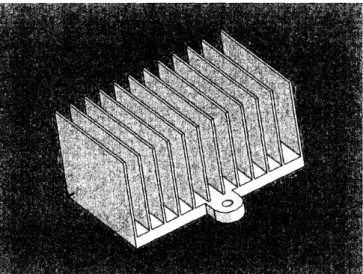
1-1 Solid model of a possible heat sink to be provided for students to test. The heat sinks will come with a variety of fin thicknesses, numbers of fins, and overall lengths. . ... ... 12 3-1 Solid model showing the heat source plate with power resistor and

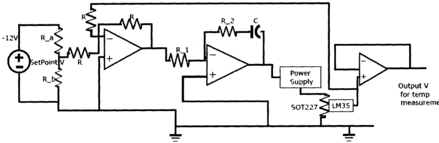
LM35 attached ... ... ... ... 20 3-2 Circuit diagram for the temperature controller. The input voltages

for the op-amps and LM35 are not shown. The power supply accepts voltages between OV and 12V. The setpoint voltage could also be set using a variable resistor (effectively providing an Ra and and Rb). . . 21 3-3 Plot showing simulation of case when the fan is off and the fin array

is unattached. Once the copper plate reaches the set point, the power supply shuts off to allow the plate to cool. Overshoot is less than 2 degrees C . .. . . .. . . . . . . . . . . . 22 3-4 Plot showing simulation of case when the fan is on and a fin array with

low resistance value is attached. The power supply cannot provide enough power to reach the setpoint temperature, so the power stays on at its maximum value and the copper plate reaches a steady state temperature lower than the set point. The temperature differences between the power resistor, copper plate, and fin array are due to the thermal resistance between them. . ... . 23

3-5 Plot showing simulation of case when the fan is on and a fin array with fairly high resistance value is attached. The power supply runs at maximum and then settles to a lower steady state once the copper plate reaches the setpoint temperature. There is no overshoot in this case. ... ... 24 3-6 Solid model showing the fin array mounted atop the copper plate, as

it will be in the duct ... . . . ... 24 3-7 Solid model of the overall box for the apparatus. . ... 25 3-8 Overhead picture of the partially-assembled, unwired apparatus. . . . 26 3-9 This picture shows the duct exit. The silicone glue used to seal the

duct is visible ... .. .... . . ... 27 3-10 This picture shows the fan attached at the entrance of the duct. . . . 27 3-11 Picture showing where the heat sink will be attached. The slot on the

left allows for attaching heat sinks of different length. . ... 28 4-1 Graph showing resistance as a function of fin array length. In this

case, base thickness is 7mmn, fin thickness is .6mm, and gap thickness is 1nm. From the graph, we chose fin lengths of 50mm, 66mm, and 90mm so that students could see that the fin array length should have some overhang beyond the heat source, but not too much overhang 30 4-2 Graph showing resistance as a function of fin width. In this case, base

thickness is 7mm, fin array length 50mm, and gap thickness is 1mm. From the graph, we chose fin widths of .4mm and .6. A fin width smaller than .4mm would have been chosen except the fins become too fragile at that thickness. ... ... ... 30 4-3 Graph showing resistance as a function of gap width. In this case, base

thickness is 7mm, fin array length 50mm, and fin thickness is .4mm. From the graph, we chose gap widths of 1mm and 1.5mnm. ... . 31

4-4 Graph showing resistance as a function of base thickness. In this case, fin array length 66mm, fin thickness is .6mrm, and gap width is 1mm. From the graph, we chose base thicknesses of 5.5mm and 10mm to go with the configuration that already was 7mrm. This will help students get an idea of the optimal base thickness for the other variables given. 31 5-1 Graph showing theoretical resistance as a function of fin array length.

In this case, base thickness is 7mm, fin thickness is .6mm, and gap thickness is 1mm. The experimental data (red stars) overlays the the-oretical prediction. ... ... ... 34 5-2 Graph showing adjusted theoretical resistance as a function of fin

ar-ray length. In this case, base thickness is 7mm, fin thickness is .6mm, and gap thickness is 1mm. The adjustment is made by adding a resis-tance value for the resisresis-tance between the power resistor and the fin array, which is determined to by approximately .0055 K/W. After the adjustment, the measured data is closer to the prediction ... . 35 A-i Fan curve for the fan used in lab. The curve B1 is the correct one. The

fan curve shows static pressure developed by the fan as a function of flow rate in cubic feet per minute. ... ... . . . 40 A-2 Graph showing theoretical resistance as a function of fin array length.

In this case, base thickness is 7mrm, fin thickness is .6mrm, and gap thickness is 1mm. The experimental data (red stars) overlays the the-oretical prediction. ... .. .... ... ... 47 A-3 Graph showing adjusted theoretical resistance as a, function of fin

ar-ray length. In this case, base thickness is 7mm, fin thickness is .6mm, and gap thickness is lmm. The adjustment is made by adding a resis-tance value for the resisresis-tance between the power resistor and the fin array, which is determined to by approximately .0055 K/W. After the adjustment, the measured data is closer to the prediction ... 47

B-i Simulink model showing the temperature controller operating on the system under normal operating conditions. . ... 50 B-2 Simulink model of heat transfer through the copper plate. ... . 50 B-3 Simulink model for the system operating under worst-case conditions. 51

Chapter 1

Introduction

1.1

2.672 Course Description

Project Laboratory in Mechanical Engineering, course number 2.672, is a laboratory subject for engineering juniors and seniors. Major emphasis is placed on the interplay between analytical and experimental methods in solution of research and development problems. Written and oral communication are strong components of the course[[2]

Over the course of the term, students complete three laboratory projects posed as engineering consulting problems. Students are instructed to design an analytical model and use the available apparatuses and measurement equipment to support the predictions of the model. In most cases, students are then requested to make recommendations regarding the design and implementation of new systems for (what is implied to be) a real-world application.

1.2

Purpose of New Experiments

The selection of experiments currently in place in the 2.672 laboratory provide inter-esting challenges for students in the class. However, it has been suggested by several faculty that it is time for new appara.ti or new experiments altogether. The field of mechanical engineering is ever-changing, with new technologies requiring a mechani-cal engineer's expertise as well as new tools and techniques at the engineer's disposal.

This is not to mention the wear and tear some of the set-ups show after years of use.

1.3

Proposed Project

As processors have been made with more and more processors and made to operate at higher and higher speeds, they have also produced more and more heat. Processors run more efficiently at lower temperatures, so fast computers depend on being able to remove heat quickly from the processor.

A popular method of removing heat from a processor is by using a heat sink. Heat sinks are finned surfaces which increase convective heat transfer by increasing the overall surface area over which such heat transfer can occur. Design of a good heat sink has evolved into something of an art form. Designers must have an understanding of air flow, extended surface approximations, and heat exchangers. Heat sinks are also subject to volume restrictions, since they must fit inside the case of a computer. In this proposed experiment, students will be asked to find an optimal configura-tion for a fin array. The setup will be a simplified version of a, standard rack-mount server (which contains a processor just like a PC does). Some simplifications will include air flow constrained to one direction, an air duct of simple, uniform cross-section, and a fin array with a limited number of parameters to change. Students will be expected to come up with a, model to predict the overall thermal resistance for a heat sink as a function of certain parameters. They will be provided with a selection of several sample fin arra-ys to test on the apparatus which they can use to verify their model. Finally, they will be asked to find the optimal parameters for a fin array of this type, which should look something like what is shown in figure 1-1.

Figure 1-1: Solid model of a possible heat sink to be provided for students to test. The heat sinks will come with a variety of fin thicknesses, numbers of fins, and overall lengths.

Chapter 2

Theory

2.1

Fins

Extended surfaces in the form of fins can be used to increase the amount of convection heat transfer by increasing the surface area over which convection occurs. They are interesting configurations to model in part because convection occurs in a direction perpendicular to that of conduction. The part of the fin closer to the high-temperature base will, naturally, be hotter than the part at the tip of the fin. Thus, greater heat transfer due to convection occurs near the base than near the tip. For an in-depth analysis of the conduction and convection equations for a fin, see Dewitt[1]. For the assumption that the tip of the fin is adiabatic, that is, if dO/dx = 0 at x = L, the temperature distribution 0(t) is given by

0 cosh m(L - x)

coshmL (2.1)

In

coshm7nL

where 0 is the difference between the temperature of the fins and temperature of the surroundings. Also, Ob is the value of 0 at the base of the fin, L is the length of the fin from base to tip, and m is given by

II t .lP (2.2)

The heat transfer rate is then given by (for a derivation see [1])

qf = M tanh mL, (2.3)

where M is given by

Ml = hPkAcOb. (2.4)

In equations 2.2 and 2.4, h is the convection heat transfer coefficient, P is the perimeter of the fin drawn in the plane parallel to the base, k is the thermal conductivity of the fin material, and A, is the cross-sectional area of the fin (Ac is assumed to be constant for the entire fin).

It is desirable to have some measure for how well a fin is doing to increase heat transfer. There are two useful measures for this: fin effectiveness and fin efficiency. Fin effectiveness is defined as the ratio of heat transfer from the fin to the heat transfer that would have occurred had there been no fin present, and it is given by the formula

sf

_(2.5)

hAcb'b

where Ar,, is the fin cross-sectional area at the base. Fin effectiveness should be greater than 1. Fin efficiency is defined as the ratio of heat transfer with the fin to the heat transfer that would occur if the entire fin were at the temperature of the base of the fin. It is given by the formula

qff _(2.6)

hAfOb

2.2

Incompressible Flow

Air flow across the fin array will be driven by a fan at one end of the duct. The fan

creates a pressure differential across the fin array which forces air to flow. While the fan curve (the relationship between volumetric air flow and pressure drop across the

fan, a characteristic the fan installed) is not linear, we model it as

Qmax

Q

=

Q

(2.7)

where Qmax is the airflow across the fan when there is zero pressure drop and APax is the pressure drop across the fan when air flow is zero.

To find the actual pressure drop across the flow rate, an equation relating the air flow to pressure drop for the fin array is needed. For this equation, we assume that all pressure drop takes place across the fin array, and we look at the gaps between fins through which air is allowed to flow. Looking at just one ga)p, we find the hydraulic diameter, DI, for the gap as

4A

Di- =

gap

(2.8)

gap

For viscous flow (flow through the small gaps between fins is certainly viscous, but we'll make sure by looking at the Reynolds number), the Darcy-Weisbach friction factor f can be used to determine the relationship between flow velocity and pressure drop [3].

f

4pz2

In (2.9), dP/dx is the pressure drop per unit length past the fin and V is the velocity of air. For the gap width used for the heat sinks, it is appropriate to use the approx-imation that the gap is a long rectangular slit. This implies the friction factor is also given by

96 96p

f 9,

(2.10)

Q(2.11)

n is the number of gaps between fins, we solve the system of equations for AP and

Q.

2.3

Heat Exchange

The calculate the overall resistance to heat transfer, we must first calculate UA, which is given by

1 1 1

S-

+

UA hiAi h,oAo

This equation assumes that the fouling factor of the heat exhanger is zero, that is, all surfaces inside the heat exchanger are clean. We can use the equation

NTU = UA (2.13)

where NTU is the number of thermal units, an engineering characteristic used to calculate the amount of heat transfer which occurs, and C,min, is the smaller of the two heat capacities of the two working fluids. In our case, C,,i, will just be the specific heat capacity of air times the air flow rate, because the hot side of the heat exchanger (the aluminum) doesn't have an actual flow rate associated with it. To calculate resistance we first must use the equation

E = 1 - e-NTU , (2.14)

where e is the fraction of actual heat transfer to the theoretical maximum calculated from the flow rate and C,,in. Tb calculate resistance, we can simply use

Roveraul =

'

ECmin

where Roveral, is the resistance to heat transfer for the heat exchanger for a given temperature difference.

2.4

Optimization

Optimization of a function over four variable can be done in a. simple way as long as the function is well-behaved. First, three of the parameters are chosen from ballpark ideas of what they should be, and the function is minimized over the remaining free variable. Then, the function is minimized over the second variable with the first variable chosen from before. The process is repeated for the other two variables, and then several more iterations are performed, each leading to a, better value for the function. The process ends when the value for the function is unchanged (or very close to unchanged) after a whole iteration.

Chapter 3

Design of Apparatus

One intent in the design of the apparatus is to convey the impression that the students are experimenting with a rack-mount server. The length and width of the box are approximately in line with a server of this type. However, the apparatus is much thicker due to the sizes of some of the electronic parts which are contained within. The height of the duct. on which the students focus most of their efforts, however, is comparable to the height of a typical rack-mount server.

3.1

Choice of Components

3.1.1

Materials Selection

The case of the server is made of Lexan, a strong, non-conducting polymer. Making the case out of Lexan, particularly the part of the case near the fin array, prevents heat transfer from the heat source to the environment via the case. In other words, having a non-metallic case makes it easy to assume that all heat transfer from the heat source to the environment occurs via the fin array.

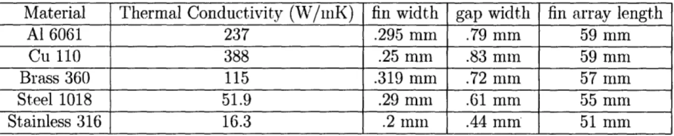
The square plate meant to represent the processor is made of copper. In a real server, the heat is generated by this pla.te itself (because the processor runs) and not by some other heat source. The choice of copper for the plate was necessary to simulate the processor as a source of hea.t as accurately as possible. Copper has a

Material Thermal Conductivity (W/nK) fin width gap width fin array length Al 6061 237 .295 mmn .79 mm 59 mm Cu 110 388 .25 mm .83 mm 59 mm Brass 360 115 .319 mm .72 mm 57 mm Steel 1018 51.9 .29 mm .61 mm 55 mm Stainless 316 16.3 .2 mmn .44 mm 51 mm

Table 3.1: Comparison of optimal geometric configurations for different heat sink materials.

high thermal conductivity which will encourage the temperature across the surface of the plate to be as uniform as possible.

3.1.2

Fin Array Material Selection

The thermal conductivity of the material that the fin array is made of has a significant effect on how well the heat sink works. We can optimize the para.meters for a heat sink just by plugging in different thermal conductivities. The results are summarized in table 3.1. This analysis encourages the use of brass as a heat sink material because it yields the thickest fins in the optimal case. Since the heat sinks will be cut on the wire EDM, it is preferable to 6061 aluminum because of the absence of non-metallic elements.

3.1.3

Heat Generation and Control Components

For the power resistor we chose the SOT227 package power resistor which will be operating at a. maximum heat dissipation rate of 144W. The power resistor is attached to the copper plate by screws, and thermal grease is applied at the interface between the two components to provide as low a thermal resistance as possible. The copper plate is machined with as good a, finish as possible to keep the small gaps between it

and the power resistor small.

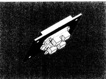
Our temperature controller depends on an accurate measurement of the temper-ature of the power resistor. For this purpose we use an LM35 tempertemper-ature sensor. However, it is not feasible to mount the sensor directly to the power resistor, so we do the next best thing. As shown in figure 3-1. the LM35 is mounted on the under

Figure 3-1: Solid model showing the heat source plate with power resistor and LM135 attached.

side of the copper plate as close to the power resistor as possilble.

3.1.4

Fasteners

For any part which is attached to the duct, we chose a button-hea-d cap screw with a hex head. The button head provides ininmaal interference with the flow of air through the duct. The hex head screws, while having the advantage of being easy to turn, also will deter stuldents from tinkering with the box, since they are less likely to be carrying hex wrenches with them than a phillip's or flat heat screwdriver that might be a feature of a Swiss Arnmy knife. The screws which are used to hold the heat sink in pllace, and which will be unscrewed by the students during the course of the lab are phillip's head screws. The other fasteners used are either button-head cap screws or special screws for the I)arts they attach (such as the fan).

3.2

Temperature Control Circuit Design

The temperature control circuit will serve two purposes. First. the experiment needs to run in stealdy state, so the controller will keep the temnperature of the copper plate constant. Second, the controller will i)revent the power resistor from overheat-ing. Overhe(ating is a risk because, if the experiment is run with the fan. off a.nd/or

ement

Figure 3-2: Circuit diagram for the temperature controller. The input voltages for the op-amps and LM35 are not shown. The power supply accepts voltages between OV and 12V. The setpoint voltage could also be set using a variable resistor (effectively providing an Ra, and and Rb).

without a heat sink attached, the time constant of the system is small and making the temperature hard to control. In order to design an appropriate temperature con-troller, a good thermal model of the system is needed. The controller will be designed to work in a worst-case scenario: with the fan off, no heat sink attached, and the cover of the duct closed. It will then be tested to make sure it works well under normal operating conditions.

3.2.1

Thermal Model

Heat will move by conduction from the power resistor to the copper plate to the fin array, and finally to the air (or straight from the copper plate to the air in the case without the fin array attached). Temperature will be measured at the copper plate, so the measured temperature will be lower than the temperature of the power resistor. The thermal model is simulated using Simulink. Graphical representations of the models, as well as the input parameters used, can be found in the Appendices. A proportional-plus-integral controller is then inserted into the Simulink model for testing. Results of the simulated tests with the controller included are shown in figures 3-3, 3-4, and 3-5.

150 100 C. =-• 50₅₀ Q. O 80 60 -. 40 E 20 0 20 40 60 80 100 time (s) 0 20 40 60 80 100 time (s)

Figure 3-3: Plot showing simulation of case when the fan is off and the fin array is unattached. Once the copper plate reaches the set point, the power supply shuts off to allow the plate to cool. Overshoot is less than 2 degrees C.

1 bU Z' 100 t-S50 o A 0 20 40 60 80 100 time (s) 50 40 a- 30 E 20 0 20 40 60 80 100 time (s)

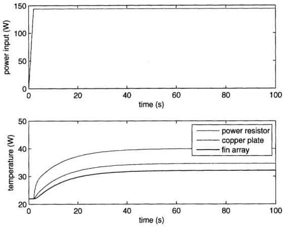
Figure 3-4: Plot showing simulation of case when the fan is on and a fin array with low resistance value is attached. The power supply cannot provide enough power to reach the setpoint temperature, so the power stays on at its maximum value and the copper plate reaches a steady state temperature lower than the set point. The temperature differences between the power resistor, copper plate, and fin array are due to the thermal resistance between thenim.

150 100 50 80 a) 60 0-40 E 20 100 time (s) 150 200 50 100 150 time (s) 200

Figure 3-5: Plot showing simulation of case when the fan is on and a fin array with fairly high resistance value is attached. The power supply runs at maximum and then settles to a lower steady state once the copper plate reaches the setpoint temperature. There is no overshoot in this case.

Figure 3-6: Solid model showing the fin array mounted atop the copper plate, as it will be in the duct.

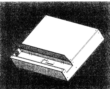
Figure 3-7: Solid model of the overall box for the apparatus.

3.3

Overall Apparatus Design

The experiment is to be presented to students in the form of a. box. This box is supposed to be of comparative size of a typical rack-rnount server, since the goal of the experiment is to optinlize a heat sink for such a server. The server box will contain a heat source meant to be of similar size, shajpe, and temperature of a the kind of processor which would run inside a server. The heat source will be simulated 1by a square copper pIlate 50ruin on each side with a power resistor on the bottom, whose power output will b)e controlled by the temperature controller described in section

3.2. Like a. typical server box, a fain will provide air flow over the heat sink. However. there are several key features not present in a server.

One feature is the presence of a hinged door on the top of the b1ox. This door allows access to the heat sink so that heat sinks can be easily interchanged. Other features inchlde devices to measure temperatlre, pressure, and power. The case of the "server" is clear to allow the students to see the electronics on the inside.

3.3.1

Sealing the Duct

When the dolor is opened, the air (luct through which air forced by the fan passes through the heat sink is opened to the atmosphere. If the fan is run in this

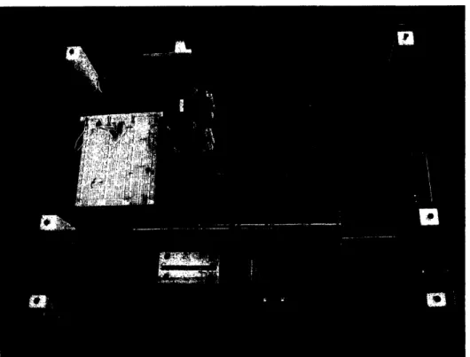
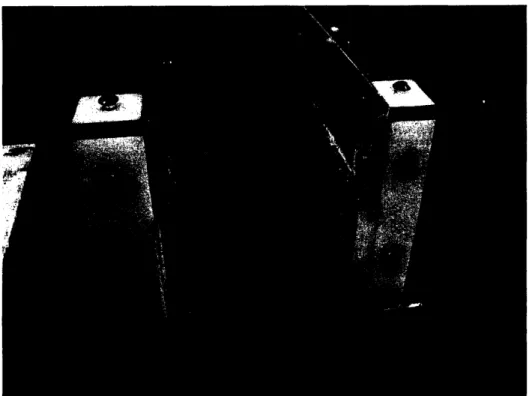
configura-Figure 3-8: Overhead picture of the partially-assembled, unwired apparatus. tion, very little air will pass through the fin array because the pressure drop required to force air through is high compared to forcing air over and around the array. Since the fan causes a pressure increase ulwind of the fin array, that part of the duct must be sealed to the atmosphere to insure that all of the pressure from the fan is used to push air through the array, and not to push air out of the duct through other exits.

There are several exits which must be sealed. One is the space between the top hinged door and the side of the duct. This exit is sealed with a foam rubber strip which, when compressed, provides a perfect seal. To keep the foam rubber compressed, we include clasps to hold the door tightly shut. Another exit is through the bottom of the duct. The heat sink is held in place by screws into the bottom, which are placed in holes in the bottom of the duct. rio prevent air from escaping there, aluminum blocks with foam rubber on the edges are placed underneath the duct to provide sinks for the screws.

Finally, for all other gaps in the walls in the duct, we apply a clear silicone glue/sealant to ensure that the duct is air-tight.

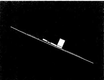
Figure 3-9: This picture shows the duct exit. The silicone glue used to seal the duct is visible.

Figure 3-11: Picture showing where the heat sink will be attached. The slot on the left allows for attaching heat sinks of different length.

3.3.2

Heat Sink Attachment

An important feature of the design involves how students will go about attaching different heat sinks to the copper plate. They must be able to ensure a solid thermal connection with the copper plate. This is done by screwing the fin array directly into the bottom of the duct.

However, ]knowing where to drill the holes in the duct is trickier, since the heat sinks will have different lengths. Instead of many different holes, a t-slot is available to screw one end of the heat sink into. Inside the t-slot is a square nut which catches the screw. This nut is free to slide back and forth in the slot. Figure 3-11 shows the result.

Chapter 4

Analytical Model

4.1

Choice of Fin Configurations for Experiment

The fin configurations were chosen so that students would have at least two heat sinks to compare with three of the variables fixed and only one varied. They were chosen by looking looking at graphs of the resistance as a fmnction of one variable. Figure 4-1 shows and example of this method.

0.164 0.162 0.16 0.158 0.156 d 0.154 F 0.152 0.15 0.148 0.146 S144 fw=.6mm gw=lmm bt=7mm 0.04 0.05 0.06 0.07 0.08 0.09 0.1 fin array length (m)

0.11 0.12

Figure 4-1: Graph showing resistance as a function of fin array length. In this case, base thickness is 7mm, fin thickness is .6mrm, and gap thickness is 1mm. From the graph, we chose fin lengths of 50mnm, 66mm, and 90mm so that students could see that the fin array length should have some overhang beyond the heat source, but not too much overhang

fl=50mm gw=lmm bt=7mm

2 3 4 5 6

fin width (m)

7 8 9 10

x 10-4

Figure 4-2: Graph showing resistance as a function of fin width. In this case, base thickness is 7rmm, fin array length 50mnm, and gap thickness is 1mm. From the graph, we chose fin widths of .4mm and .6. A fin width smaller tha.n .4mm would have been chosen except the fins become too fragile at that thickness.

.71 /7 E E

-fl=50mm fw=.4mm bt=7mm 0.24 0.22 0.4 0.6 0.8 /// 1 1.2 1.4 1.6 1.8 gap width (m) _{x 10}: 1

Figure 4-3: Graph showing resistance as a function of gap width. In this case, base thickness is 7rnim, fin array length 50(nun, and fin thickness is .4mm. From the graph, we chose gap widths of mmin and 1.5mnm.

fl=66mm fw=.6mm gw=1mm - - --T - -u. 158 0.156 0.154 0.152 .n 0.15 2) 0.148 0.146 0.005 0.01 base thickness (m) 0.015

Figure 4-4: Graph showing resistance as a fumnction of base thickness. In this case, fin array length 66rnm, fin thickness is .61nin, alnd gap width is lnunn. Froml the graph, we chose base tlhicknesses of 5.5mm and 10nmin to go with the configuration that already was 7mm. This will help students get an idea of the optimal base thickness for the other varialles given.

E -- t.-v_ -··--r -rh

Chapter 5

Simulated Results

The following results were simulated in MIATLAB by taking the predicted results and adding a randomly distributed error term. For the resistance measurements, an addition constant term was added to each resistance because of resistance from the copper plate to the fin array. In the actual experiment, the theoretical resistance will be subtracted from the experimental resistance to calculate this extra resistance from the thermal grease. This could also be calculated from the properties of the thermal grease, but the thickness of the grease between the surfaces is unknown due to variation in. how well the students apply it and how good the surface finish is. Also note that the predictions were based on Aluminum fins, the material of the first fin array, but the fins used in the experiment will probably be brass but could be some other material.

5.1

Pressure Drop

The pressure readings provide a quick check of the incompressible flow aspect of the model. Since, theoretically, the pressure drop is just a function of the fan curve and the duct geometry (primarily the fin gap geometry), confirming the pressure model correct will give a fairly accurate volumetric flow rate.

The pressure data, compared to the pIredicted values, is printed in table 5.1. Some of the measurements have significant error, with the majority of the measured

Heat Sink Number Measured Pressure (Pa) Predicted Pressure (Pa) Percent Diff. 1 53.6 54.6 1.8

2

25.8

25.8

-0.03

Table 5.1: Comparison of measured to predicted pressure drops for each heat sink. Heat Sink Number Measured Resistance (K/W) Predicted Resistance Percent Diff.

1 0.206 0.152 40.8 2 0.263 0.208 28.7 3 0.209 0.154 41.3 4 0.200 0.145 41.4 5 0.205 0.150 41.4 6 0.200 0.145 40.7 7 0.201 0.146 39.6

Table 5.2: Comparison of measured resistance to p)redicted resistance values for the different heat sinks. The mneasured resistance was calculated by dividing steady state temperature by steady state power.

pressures lower than the predicted values. A possible explanation for this is that the fins in the fin arrays are not perfectly straight, so some of the spaces between fins are larger than they should be, letting more air pass through. It is unclear whether the fins are bent because of damage to them or because of the way they were manufactured.

5.2

Resistance

Resistances are not measured directly. Instea~d power dissipation and temperature is measured. Resistance is calculated using the difference in temperature between the copper plate and room temperature. Tables 5.2 and 5.3 summarize the differences between measured and predicted values.

H.S. Number Measured Resistance (K/W) Predicted Res (adjusted) Percent Diff. 1 0.206 0.207 3.41 2 0.263 0.263 1.89 3 0.209 0.209 4.16 4 0.200 0.200 2.51 5 0.205 0.205 3.55 6 0.200 0.200 2.14 7 0.201 0.201 1.52

Table 5.3: Comparison of measured resistance to predicted resistance values for the different, heat sinks. In this case, the predicted values have be adjusted to include resistance between the power resistor and the fin array. All the predicted resistances simply have a constant value of 0.055K/1 , aadded to them.

0.19

0.16

fw=.6mm, gw=lmm, bt=7mm

,

0.05 0.06 0.07 0.08 0.09

fin array length (mm)

0.11 0.12

Figure 5-1: Graph showing theoretical resistance as a function of fin array length. In this case, base thickness is 7nim, fin thickness is .6mm, and galp thickness is lmm. The experimental data (red stars) overlays the theoretical prediction.

_,· ~_~~_ ~_~_,,

--fw=.6mm, gw=lmm, bt=7mm 218 0.216 0.214 0.212 0.21 0.208 a 0.206 0.204 0.202 0.2 A ion 0.05 0.06 0.07 0.08 0.09 0.1 0.11 0.12 fin array length (mm)

Figure 5-2: Graph showing adjusted theoretical resistance as a function of fin array length. In this case, base thickness is 7mm, fin thickness is .6mm, and gap thickness is 1mm. The adjustment is made by adding a resistance value for the resistance between the power resistor and the fin array. which is determined to by approximately .0055 K/W. After the adjustment, the measured data is closer to the prediction.

?4

C.t

Chapter 6

Conclusions

6.1

Direction for Further Work

Since the heat sinks have not been tested, it is unclear whether or not they give good enough results in reality that will allow student to understand how varying different parameters affects the resistance. If the reality doesn't match up with the model closely enough, it might be advisable to make a new batch of heat sinks which conveys the best information to the students.

6.2

Suggestions for Improvement of Apparatus

The case suffers from imprecise construction, and has some aesthetic and structural problems which could be fixed by a rebuild. For example, the outer walls of the box don't line up properly, and the duct is held together more by glue than by the L-shaped braces that attach the bottom of the duct to the sides.

The temperature sensors are not good enough to measure the bulk temperature of exiting air because the of the temperature variation across the profile of the air flow. Maybe more sensors could be added and their outputs averaged.

The temperature controller is currently wired on a breadboard. It should be eventually done on a. printed circuit board for a. more permanent solution.

The screws that hole the copper plate to the bottom of the duct should be counter sunk so that dimples don't need to be drilled in the bottoms of hea.t sinks.

Appendix A

Sample 2.672 Lab Report

This appendix presents a demonstration lab writeup which might be written by a 2.672 student assigned to this experiment. Because it uses simulated data for heat sinks made of aluminum instead of brass and for parameters not actually used in their construction, it should not be used as a model lab report.

A.1

Abstract

Fans and heat sinks are a popular method of keeping computer processors cool. In this report, certain parameters of a heat sink fin configuration are optimized for a particular rack-mount server. A model is developed to analyze how fin thickness, fin spacing, base thickness, and heat sink length affect the resistance to heat transfer of the fin array. Several different heat sinks are used to verify tile model, and the optimum configuration is found using numerical optimization techniques. For the given fan specifications and duct dimensions, the optimum configuration is given by an array length of 59 mm, a fin thickness of .30 mm, a fin spacing of .79 inm, and a base thickness of 6.5 mm. The model predicted the experimental results with less than 15 percent error (in the resistance measurement).

A.2

Introduction

Computer processors generate heat during operation, but their performance suffers when they operate at too high temIperatures. They can even be destroyed if they overheat too much. In order for processors to run at high speeds, they need to be kept at low temperature by some sort of cooling system. One particular kind of cooling system, the kind investigated in this report, uses a heat sink with forced convection.

Heat sinks are finned surfaces which increase convective heat transfer by increasing the overall surface area over which such heat transfer can occur. Design of a good heat sink has evolved into something of an art form. Designers must have an understanding of air flow, extended surface a.pproximations, and heat exchangers. Heat sinks are also subject to volume restrictions, since they must fit inside the case of a computer. The purpose of this lab is to design an optimal hea.t sink for a given processor size, air duct, and fan characteristic. The material of the heat sink is restricted to aluminum (6061 alloy), but there are four geometric parameters which

A.3

Apparatus and Procedure

The apparatus is made of clear Lexan and contains a. heating element that must be kept cool. The system to be cooled consists of a processor of square shape, 48 cm on a side, situated in an air duct of a rack-mount server. On one end of the duct is a fan with fan curve shown in figure A.3.1; the other end of the duct is open to the atmosphere inside the server room. The duct is about 60 cm long, and its cross-section is approximately 8 cm by 4 cm (width and height, respectively). In order to investigate the system, a model of the server box is available, with a power resistor mounted to a copper plate to simulate the processor's heat generation.

O₀₀ 3 1.2 1 0.8 a0 0.6 0.4 0 Airflow (CFM)

Figure A-1: Fan curve for the fan used in lab. The curve B1 is the correct one. The fan curve shows static pressure developed by the fan as a function of flow rate in cubic feet per minute.

A.3.1

Sensors and Measurement

Power provided to the resistor and the temperature of the copper plate have analog outputs provided. Temperature is measured by an LM35 temperature sensor, which is already calibrated to give .01 Volts per degree Celsius. Pressure drop across the fin array is measured by a PC Board Mount pressure sensor with a range of -5 to 5 inches of H20.

A.3.2

Procedure

Data was collected by attaching a heat sink to the duct and copper plate, closing the top flap, turning on the fan, and turning on the power to the resistor. After about two minutes, the temperature and power levels out to a steady state, and the values for power, temperature, and pressure drop are recorded. The power to the resistor is turned off and the apparatus is allowed to cool before removing the hea.t sink. A different heat sink is attached and the procedure is repeated.

A.4

Theoretical Analysis

A.4.1

Fins

Extended surfaces in the form of fins can be used to increase the amount of convection heat transfer by increasing the surface area over which convection occurs. They are interesting configurations to model in part because convection occurs in a direction perpendicular to that of conduction. The part of the fin closer to the high-temperature base will, naturally, be hotter than tile part at the tip of the fin. Thus, greater heat transfer due to convection occurs near the base tha.n near the tip. For an in-depth analysis of the conduction and convection equations for a fin, see Dewitt[1]. For the assumption that the tip of the fin is adiabatic, that is, if dO/dx = 0 at x = L, the

temperature distribution 0(t) is given by

cosh m(L - x)

/0, = coshmL

_coshmi.L

m = hP/kA-. (A.2)

The heat transfer rate is then given by (for a derivation see [1])

qf = A tanh mL, (A.3)

where M is given by

Ml - hPkABO,. (A.4)

In equations A.2 and A.4, h is the convection heat transfer coefficient, P is the perime-ter of the fin drawn in the plane parallel to the base, k is the thermal conductivity of the fin material. and A, is the cross-sectional area of the fin (A, is assumed to be

constant for the entire fin).

It is desirable to have some measure for how well a fin is doing to increase heat transfer. There are two useful measures for this: fin effectiveness and fin efficiency. Fin effectiveness is defined as the ratio of heat transfer fromn the fin to the heat transfer that would have occurred had there been no fin present, and it is given by the formula

f q _(A.5)

hAc,,Ob

where Ac,b is the fin cross-sectional area. at the base. Fin effectiveness should be greater than .. Fin efficiency is defined as the ratio of heat transfer with the fin to the heat transfer that would occur if the entire fin were at the temperature of the base of the fin. It is given by the formula

qf (A.6)

hAfOb"

A.4.2

Incompressible Flow

Air flow across the fin array will be driven by a fan at one end of the duct. The fan creates a pressure differential across the fin array which forces air to flow. While the fan curve (the relationship between volumetric air flow and pressure drop across the fan, a. characteristic the fan installed) is not linear, we model it as

Q

=

where Q,,,x is the airflow across the fan when there is zero pressure drop and A Pmax is the pressure drop across the fan when air flow is zero.

To find the actual pressure drop across the flow rate, an equation relating the air flow to pressure drop for the fin array is needed. For this equation, we assume that all pressure drop takes place across the fin array, and we look at the gaps between fins through which air is allowed to flow. Looking at just one gap, we find the hydraulic

diameter, Dh for the gap as

D

=

(A.8)

Pgap

For viscous flow (flow through the small gaps between fins is certainly viscous, but we'll make sure by looking at the Reynolds number), the Darcy-Weisbach friction factor f can be used to determine the relationship between flow velocity and pressure drop.

f

In (A.9), dP/dx is the pressure drop per unit length past the fin and P9 is the velocity of air. For the gap width used for the heat sinks, it is appropriate to use the approx-imation that the gap is a long rectangular slit. This implies the friction factor is also given by

96 96p

f , (A.10)

Re pairODi,

where Re is the Reynolds number. p, is the viscosity of air, and pair is the density of air. From the friction factor equation and the fan curve, we can solve for the flow rate and pressure drop through the fin array. Noting that

Q

where Agap is the gap width times the distance from the base of the fin to its tip and

n is the number of gaps between fins, we solve the system of equations for AP and

Q.

A.4.3

Heat Exchange

The calculate the overall resistance to heat transfer, we must first calculate UA, which

is given by

1 1 1

S= A- h (A.12)

This equation assumes that the fouling factor of the heat exhanger is zero, that is, all surfaces inside the heat exchanger are clean. We can use the equation

UA

NTU = ' (A.13)

where NTU is the number of thermal units, an engineering characteristic used to calculate the amount of heat transfer which occurs, and C,,in is the smaller of the two heat capacities of the two working fluids. In our case, C,,in will just be the specific heat capacity of air times the air flow rate, because the hot side of the heat exchanger (the aluminum) doesn't have an actual flow rate associated with it. To calculate resistance we first must use the equation

E = 1 - - NTi , (A.14)

where c is the fraction of actual heat transfer to the theoretical maximum calculated from the flow rate and Cmi,. To calculate resistance, we can simply use

Rocvr.au = - (A.15)

where Rovera,, is the resistance to heat transfer for the heat exchanger for a given temperature difference.

A.4.4

Theoretical Predictions

Predictions for the resistance of each heat sink can be found by using the three models discussed above. The flow rate is calculated by finding the hydraulic diameter for the gaps between the fins, which is given approximately by Dh = 2 * gw, where guw is the

fin spacing. The hydraulic diameter and fin array length gives a friction factor, which can then be used to construct a pressure vs. flow rate curve. The intersection of this curve with the fan curve yields the actual flow rate and pressure drop.

Similarly, the convection heat transfer coefficient h. can be calculated from the geometry of the fins. The fin equations are used to find an effective heat transfer

Heat Sink Number Measured Pressure (Pa) Predicted Pressure (Pa) Percent Diff. 1 53.6 54.6 1.8 2 25.8 25.8 -0.03 3 63.0 60.2 -4.6 4 63.7 73.8 14 5 85.3 90.9 6.1 6 58.3 71.4 18 7 73.9 79.2 6.7

Table A. 1: Comparison of measured to predicted pressure drops for each heat sink.

coefficient and fin efficiency, and then the array overhang is modeled as a fin with the same thickness as the base thickness to further refine out efficiency calculation. Finally, the heat exchanger equations are used to calculate the overall resistance for the fin array.

A.5

Results and Discussion

A.5.1

Pressure Drop

The pressure readings provide a quick check of the incompressible flow aspect of the model. Since, theoretically, the pressure drop is just a function of the fan curve and the duct geometry (primarily the fin gap geometry), confirming the pressure model correct will give a fairly accurate volumetric flow rate.

The pressure data, compared to the predicted values, is p)rinted in table A.1. Some of the measurements have significant error, with the majority of the measured pressures lower than the predicted values. A possible explanation for this is that the fins in the fin arrays are not perfectly straight, so some of the spaces between fins are larger than they should be, letting more air pass through. It is unclear whether the fins are bent because of damage to them or because of the way they were

Heat Sink Number Measured Resistance (K/W) Predicted Resistance Percent Diff. 1 0.206 0.152 40.8 2 0.263 0.208 28.7 3 0.209 0.154 41.3 4 0.200 0.145 41.4 5 0.205 0.150 41.4 6 0.200 0.145 40.7 7 0.201 0.146 39.6

Table A.2: Comparison of measured resistance to predicted resistance values for the different heat sinks. The measured resistance was calculated by dividing steady state temperature by steady state power.

H.S. Number Measured Resistance (K/W) Predicted Res (adjusted) Percent Diff.

1 0.206 0.207 3.41 2 0.263 0.263 1.89 3 0.209 0.209 4.16 4 0.200 0.200 2.51 5 0.205 0.205 3.55 6 0.200 0.200 2.14 7 0.201 0.201 1.52

Table A.3: Comparison of measured resistance to predicted resistance values for the different heat sinks. In this case, the predicted values have be adjusted to include resistance between the power resistor and the fin array. All the predicted resistances simply have a constant value of 0.055K/tW added to them.

A.5.2

Resistance

Resistances are not measured directly. Instead power dissipation and temperature is measured. Resistance is calculated using the difference in temperature between the copper plate and room temperature. Tables A.2 and A.3 summarize the differences between measured and predicted values.

A.6

Conclusions

It is not possible to get an exact value of the resistance of the fin array due to unknown resistances between the power resistor and the heat sink. However, this does not affect the possibility of minimizing the resistance, since each measured resistance is off by a constant value (assuming the thermal grease was applied correctly. The optimal

0.21, 0.19 ý 0.18 ,n 0.17 a 0.16 0.15 fw=.6mm, gw=lmm, bt=7mm - --- --- rI ---- r---0.05 0.06 0.07 0.08 0.09 0.1 0.11 fin array length (mm)

0.12

Fignre A-2: Graph showing theoretical resistance as a fiunction of fin array length. In this case, base thickness is 7mrm, fin thickness is .61nn, and gap thickness is 1mm.

rfhe experimental data (red stars) overlays the theoretical prediction.

fw=.6mm, gw=lmm, bt=7mm

-- -- r . ....

K

*

0.05 0.06 0.07 0.08 0.09

fin array length (mm)

0.1 0.11 0.12

Figure A-3: Graph showing adjusted theoretical resistance a.s a. function of fin array length. In this case, base thickness is 7mTm, fin thickness is .6mm, anrd gap thickness is 1mrm. The adjustment is made 1•y adding a resistance value for the resistance between the power resistor and the fin array, which is determined to by approximately .0055 K/W. After the adjustment, the measured data is closer to the prediction.

0.218 0.216 0.214 0.212 0.21 0 0.208 a 0.206 0.204 0.202 0.2 0(149 ---Cý --~.___.__ I _~_.1__~__ I L~ _).12 ^^'^ E --- I~ __.L __.I_. II

resistance is given by and fin array length of 58.7 mm, a fin width of .295 mm, a gap width of .786 nun, and a base thickness of 6.53 iun. The resistance of such an array would be .1370 K/W, good enough to dissipate 144 W at a temperature of only 42 degrees Celsius.

Appendix B

Simulink Models

The Simulink program is a part of the MATLAB package, which is available to MIT students who are connected to the internet through the MIT network. Simulink provides a stateflow approach to modeling. Objects have inputs and outputs, and

lines connect the output from one object to the input of another.

The Simulink models shown herein model the controlled temperature and power dissipation of the resistor, plate, and fin array system. The model in figure B is for the case when the heat sink is in place, the duct is closed, and the fan is running.

The large blocks in B refer to smaller systems. One such system, the one describing heat transfer through the copper lpla.te, is shown in figure B.

Figure B shows the Simulink model for our worst-case scenario in terms of con-trolling the temperature: the duct closed, the fan off, and no heat sink in place. Note that it doesn't have the block to model the hea.t sink that figure B has.

Fin Array

Figure B-1: Sinmulink model showing the temperature controller operating on the system under normal operating conditions.

Fin Array Temp Tfa

Figure B-2: Simulink model of heat transfer through the copper plate.

Ambient Temperature

Appendix C

MATLAB Code

function resistance = heat_sinkresistance(fin_length, ..

fin_width, ..

gapwidth, ..

base_thickness)

%apparatus variables

heat_source_length=.04572; %m for AMD athlon processor

heat_source_width=.04572;

%http: www. amd. comrn us- en assets content_ type white_papers•_and techdocs 23792.pdf

duct_height=.04; %om Lo

duct_width=.08; %mr

maxpressure_drop=250; %Pa (modeled fan curve pressure drop)

max_flowrate=.01165; %m3s (modeled fan curve volumetric .flow rate)

airtemp=273+22; %K

%material constants

k=237; % W (m*K) from http:en. wikipcdia. orqwikiAlumrrinium

mu=1.8e-5; %Pa*s 20 c_p_air=1012; %J(kg*K) specific heat of air

k_air=0.0257; %W(m*K)

%calculation of h

a=gap_width;

b=d uct_ height- base_thickness; b.a;

Dh=4.*(a.*b).(2.*a+2.*b);

%Dh=a2; %true when b>>a, but we dont need to make this assumption

30

Nu=7.54; %Nu=hDk, assuming constant surface temp and b>>a f_ReDh==96; 7assuming b>>a

h=Nu.*k_air.Dh;

%ceiling because we can often let iilosethe fin array with a thinner fin

num_fins=ceil(duct_width.(finwidth+gap_width));

%calculation of pressure drop and flow rate from fan, curve and friction

%factor 40

flow_rate=max_pressure_drop. ((f_ReDh .2.*mu.*fin length). (Dh.2.*a.*b.*num_fins)+ maxpressure_drop. (maxflowrate));

pressuredrop=fReDh.2. *mu. *fin length.(Dh.2. *a.*b. *num fins).*flowrate;

velair=:flowrate.(num_fins.*b.*gap_width); Re=rho.*vel_air.*Dh.mu;

%calculation of fin efficiency

Ac=fin_length.*fin_width; 50

fin_effectiveness=sqrt(k.*P.(h.*Ac)); m=sqrt(h.*P.(k.*Ac));

L=b;

finefficiency=tanh(m.* L).(m.*L);

%calculation of overall heat transfer coefficient

Af=2.*(fin_length.*b).*num_fins; %total fin surface area

Aeb=(fin_length.*gap_width).*(num_fins-1); %surface area of exposed base

60

%equivalent to Aeb(Af+Ae-b) +finefficiency*A4f (Af+Aeb)

overallfinefficiency= 1- Af.(Af+Aeb).*( -fin_efficiency);

%calculate the efficiency of base plate as if it were a fin of thickness %basethickness and it had an h=h_cff

heff=(h.*gap width+(fin-efficiency.*h.*(2.*fin -ength.*b).(fin-width.*fin-length)).* fin_width).(finwidth+gap_width);

mbase_.platel=sqrt(h_eff. * (2. *(heat_source_width) +

2.*base_thickness).(k.*((heat_source_width).*basethickness))); 70

mbaseplatew=sqrt(h efF.*(2.*(heat source_length)+

2.*base_thickness). (k. *((heat_source_Iength). *basethickness)));

Lbase_platel=(a bs(finlength- heat_source_length) + (fin_length- heat_source_length ))2; L_base_platew=(abs(duct_width -heat_sou rcewidth)+ (ductwidth - heatsou rcewidth))4;

baseplate_efficiencyl=tan h( m base_plate_ .*L_base_plate_). (m_baseplate_l.* Lbase_plate_I);

base plateefficiencyw=tan h(m_base_platew.*L_ baseplatew). (m baseplatew.*

%calculate UA 80

UA=h_efF.*(heat_source_width. * heat-source length);

UA=UA+h eff. *base_plate_efficiency w. *(ductwidth-heatsourcewidth).*heat_sourcelength;

UA=UA+h eff. *baseplateefficiency I.*(f in-ength-heat-source-length).*heat-sourcewidth; UA=UA+h eff.*base_plate_efficiency_ .*baseplateefficiencyw. *(finlength

-heat_source_length).*(duct_width-heatsource-width);

%because the temperature of the aluminum doesnt change much over the %length of the fin

C_m in=c_p_air. *flow_rate. *rho;

NTU=UA.C_min; so

epsilon=1-exp(-NTU); %from Incropera Dewitt p6 8 9, assuming Cr=O;

%optimization. m

%run this script to find the optimal parameters for a heat sink. %it can be used for different materials by commenting/uncommenting %the approprate lines.

fl=50e-3; fw=.63e-3; gw=le-3; bt=7e-3;

%resist==heatsink-resistance2copper(fl, fw, gw, bt); %resist==heaLsinkresistan7ce2brass (fl, .fw, gw,bt) % resist=heatsinkresistance2steel(fl,fw, gw, bt)

resist =heat _sinkresi st ance2stainless (fl,fw,gw.bt ) to oldres=10;

while oldres-resist > le-6 oldres=resist; gws=le-5: le-6:2*gw; % res=lheaLsink-resistance2copper(flfw, gws, bt); % res=heatsinkresistance2brass (fl,fw, gws. bt); % res=heatsinkresistannce2stcel(flfw, gws, bt); res==heatsinkresistance2stainless(flfwgws. bt);

index=find (res==min (res)); 20

gw==gws(index)

fls=:49e-3:1e-5:fl+10e-3;

% res=heaLsinxkresistance2copper(fis,fw, gw, bt); % res= heatsinkresistance 2brass (fls,fw. gw, bt); % res=heatsinkresistance2steel(fls,fw, gw, bt);

res== heat _sink_resistance2st ainless (fls,fw,gw,bt); index=find(res==min(res));

plot (fls,res)